1

1

September 2011 Doctor of Philosophy

J. Anthony Tyson David Wittman, Christopher Fassnacht 3

B.A. (University of California, Berkeley) 2004

Physics Davis

Modeling Techniques for Measuring Galaxy Properties in Multi-Epoch Surveys

Data analysis methods have always been of critical importance for quantitative sciences. In astronomy, the increasing scale of current and future surveys is driving a trend towards a separation of the processes of low-level data reduction and higher-level scientific analysis. Algorithms and software responsible for the former are becoming increasingly complex, and at the same time more general – measurements will be used for a wide variety of scientific studies, and many of these cannot be anticipated in advance. On the other hand, increased sample sizes and the corresponding decrease in stochastic uncertainty puts greater importance on controlling systematic errors, which must happen for the most part at the lowest levels of data analysis. Astronomical measurement algorithms must improve in their handling of uncertainties as well, and hence must be designed with detailed knowledge of the requirements of different science goals. In this thesis, we advocate a Bayesian approach to survey data reduction as a whole, and focus specifically on the problem of modeling individual galaxies and stars. We present a Monte Carlo algorithm that can efficiently sample from the posterior probability for a flexible class of galaxy models, and propose a method for constructing and convolving these models using Gauss-Hermite (“shapelet”) functions. These methods are designed to be efficient in a multi-epoch modeling (“multifit”) sense, in which we compare a generative model to each exposure rather than combining the data from multiple exposures in advance. We also discuss how these methods are important for specific higher-level analyses – particularly weak gravitational lensing – as well as their interaction with the many other aspects of a survey reduction pipeline.

Chapter 0 Introduction and Motivation

1 From Images to Catalogs

Vision is the most powerful and well-developed of the human senses, and our brains excel at difficult pattern matching and image analysis tasks that still vex our most advanced computer algorithms. In many scientific disciplines, however, automated image processing techniques already perform better than the human eye in many respects; while the human eye excels at discovery and classification, computers are far more quantitative and repeatable. Almost all automated image analysis can be seen as a form of modeling and/or image reconstruction. Algorithms generally attempt to divide an image into parts they can separately understand, and model these independently in such a way that we can build a theoretical approximation to the original image. The success of such approaches depends crucially on our ability to define reasonable models and methods to constrain their free parameters with the data. Astronomical images are vastly simpler than most of the images our brains process daily, and are usually less complex than most scientific imaging in other fields, such as medicine or the earth sciences. Most of the night sky is dark, and while upon closer inspection it is full of billions of faint objects, we can represent the vast majority of these individually using one of two models, one for stars and one for galaxies. However, astronomical images also have a much lower signal-to-noise ratio than images in other disciplines, so while it is relatively easy to build a model-based reconstruction of the sky that roughly resembles an image, it can be much harder to validate that those models reflect reality, and to solve the inverse problem of constraining those models using the available data.

Unlike the beautiful images produced for press releases and public outreach, raw astronomical data is rarely pretty. In fact, the most scientifically interesting data is often the ugliest in its raw form, where detector artifacts and distortions, noise, resolution limits, and foreground and background contaminants conspire to make the signal of interest difficult to extract. In the current era of large, public surveys, much of the data reduction must be done without a specific scientific signal in mind; the goal is to generate catalogs that allow a wide range of studies without recourse to the raw image data. While it will always be important for astronomers to fully understand the processes that generate high-level data products like catalogs, the technical skills involved in developing survey data reduction pipelines have diverged somewhat from the more traditional astronomical skills involved in analyzing catalog data and obtaining and reducing smaller, more targeted observations. We should not consider the first set of skills the domain of engineers and statisticians, however, as many of the problems are unique to astronomy, and astronomers have a long history of developing algorithms that are useful even beyond their field. Indeed, many subfields of astronomy, such as weak gravitational lensing, clearly require both large surveys and the close attention of practitioners to the pixel-level data reduction algorithms, though most may be less interested in the technical details of how those data reduction algorithms are implemented.

1 Early Automated Data Reduction

The first modern wide-area astronomical surveys were carried out in the 1950s at the Palomar and Lick Observatories in California, covering essentially the entire northern sky. Copies of the Palomar Observatory Sky Survey (POSS) were made available for purchase, giving birth to a public survey in which outside researchers could make use of the data in ways unforeseen by the original researchers. Data access was limited to the plates; there were no official catalogs, and most analysis was done by eye. George Abell’s original catalog of 2712 galaxy clusters, published in 1958 and based on a visual inspection of the POSS plates, is still in wide use today as a definitive list of massive, nearby clusters. A large catalog of galaxies counts from the Lick survey, published by Shane & Wirtanen (1967), was notable in marking a transition to a more statistical approach to astronomy; unlike the catalogs of mainly bright and well-resolved galaxies published earlier, the Lick survey enabled studies of the spatial distribution of faint galaxies, revolutionizing our perspective on the structure of the universe.

Producing catalogs from these surveys and their successors by eye was an incredibly labor-intensive process, however, and the early 1970s saw the first computer-based methods for automated astronomical data analysis. These depended on plate scanning machines, which were almost immediately capable of much more precise measurements than the human eye. More importantly, automated measurements were far more repeatable and consistent, eliminating a major source of human bias in the process of measurement. Software for detecting, segmenting, and measuring the properties of stars and galaxies continued to be developed throughout the 1970s, and was ultimately packaged into well-defined, widely-used software systems such as FOCAS (Jarvis & Tyson, 1981) and IRAF in the early 1980s. Throughout the 1980s, NASA took the lead in advocating digital public data, releasing public images and catalogs from its space-based telescopes and digitizing photographic plate surveys. The latter culminated in the Digitized Sky Survey, a scanned version of POSS and its successors in both the northern and southern hemispheres.

2 Modern Surveys and “User Friendly” Data

The primary technological limitation throughout the 1970s and 1980s was detector technology; photographic plates suffered from nonlinearities, distortions, and low throughput, and early arrays of photodiodes or photomultiplier tubes suffered from poor resolution and photometric and astrometric instability. This changed as larger and less-noisy CCD arrays became available throughout the 1980s and 1990s, and while CCD-based surveys have yet to match the all-sky coverage of photographic plates at comparable resolutions, even early generation CCDs produced much higher-quality data with a much larger dynamic range over smaller areas. A key feature of CCD observations was that systematic effects due to the detector could be calibrated out through repeated observations; QE variations across the chip did not change between observations, and thus could be separated from variations in the sky background. This enabled observations to ultimately go much deeper, as multiple exposures could be combined without being limited by a irreducible systematic noise floor(Tyson, 1986). Deeper, higher-quality data demanded improved data reduction algorithms and software, and enabled qualitatively new types of measurements (such as weak gravitational lensing) that were not possible with photographic plates.

Telescopes with CCD cameras and similar infrared detectors started to survey large areas of the sky in the middle and late 1990s. Surveys such as the 2-Micron All Sky Survey (2MASS, Skrutskie et al. 2006) and the Sloan Digital Sky Survey (SDSS, York et al. 2000) necessitated a more “user-friendly” approach to public data, in which more and more of the low-level data reduction was done by the survey collaboration and facility, with less done by public “users” of the data. This allowed many reduction steps to be done more infrequently, with the results published to the community in the form of regular data releases. It also allowed the algorithms to be tuned by specialists who understood the data best, freeing other astronomers to focus more on higher-level science questions. Meanwhile, easy-to-use software packages – most notably SExtractor (Bertin & Arnouts, 1996), a successor to FOCAS – became standards that defined algorithmic choices for many individual data reduction tasks.

The SDSS SkyServer database (Szalay et al., 2000) takes this user-friendly public data concept one step further, providing a queryable database full of measurements that are more carefully tuned and calibrated than could be achieved independently using available software like SExtractor. While downloading and using the SDSS image data directly is no longer prohibitively difficult from a technological standpoint, the quality of the catalogs and the ease with which users can access them have made image access less important. Many papers based entirely on SDSS data use only the public catalogs, and others that do use the SDSS images or data from other telescopes rely heavily on the database for sample selection, high-quality measurements, and calibration. We cannot attribute the success of the SDSS entirely to its data-reduction and public interface advantages; it is, after all, the largest optical survey to date in many respects, and it makes use of world-class instruments. But it is fair to state that the usefulness of the survey would have been greatly diminished without the quality or the ease-of-use of its public catalogs.

3 Future Challenges

The data reduction challenge will become even more acute in the near future, with the advent of even larger surveys such as that of the Large Synoptic Survey Telescope (LSST, Ivezic et al. 2008). The challenge here is both technical and scientific. The sheer data volume means the catalogs must be more generically useful, because it is simply impractical to provide the computing power or network bandwidth for most users to operate on the pixels directly, and the official nightly and yearly processing must be highly optimized and highly parallelized to keep up with the torrent. Meanwhile, the vastly increased survey volume makes control of systematic errors much more important; systematic effects that could previously be ignored because they were smaller than the measurement uncertainties must now be addressed. Algorithms must also be improved because future surveys will go to much lower surface brightness levels, forcing us to model faint features that were previously in the noise – while we have gone deeper in small areas of the sky, the LSST will cover half the sky at a depth comparable to all but the deepest space-based observations, and many of the methods used for low surface brightness studies on narrow surveys (especially space-based surveys) will not be usable at those scales. Furthermore, most of the next generation of surveys are purely photometric, while the current state of the art, SDSS, is also a spectroscopic survey. To bring much of the SDSS science to LSST scale, we must improve methods (such as photometric redshift techniques) that can make up for the lack of spectroscopic data. Increased reliance on these algorithms may put additional requirements on our basic data reduction algorithms as well. Finally, for the first time it will become completely impractical for data quality analysis to rely heavily on human inspection; we must have automated ways to flag both expected and unexpected errors in the data.

One of the most fundamental changes from SDSS to the surveys that are now coming online is that almost all current and future surveys are multi-epoch surveys. In some cases, this means each piece of sky is observed perhaps 5-10 times in each bandpass. For LSST, the average patch of sky may be observed 200 times in each band, and some smaller areas may have thousands of overlapping exposures. There are some indications from current medium-size surveys that this large difference between the single-exposure depth and the full survey depth requires a qualitatively different approach to object measurement. Rather than combine images and perform measurements on a coadd, we may need to model all exposures simultaneously. This procedure, called “multifit” within the LSST collaboration, is not new to astronomy – but in the past it has been mostly limited to small areas, and generally used only on relatively easy-to-model point sources. Early work in multifit shear estimation by Roat et al. (2004) and Tyson et al. (2008), in addition to coining the term, demonstrated notable improvements under certain conditions. The multifit approach is formally superior when speed is not a concern, but it remains to be seen whether a more careful coadd-based approach can also meet the requirements of future surveys.

2 Inverse Problems and Generative Models

1 Astronomy as an Inverse Problem

While we can improve detectors and build our telescopes at better sites to minimize the contamination of the scientific signals we are interested in, astronomy is inherently an observational science. We usually do not have the luxury of designing an experiment to isolate an interesting effect or control systematic errors by (for instance) modulating the source; we are always limited at some level by what nature gives us, and we must infer the signal of interest from that data.

In this situation, the only recourse is to model these contaminants, from purely observational details like out-of-focus optics, to inconveniently-positioned celestial bodies that may obscure more fascinating ones. Sometimes these models are based on a physical understanding of the contamination process; often they are derived from our knowledge of how the process affects other aspects of our data – we can use stars to constrain a point spread function (PSF) model, for instance. With an appropriate model, we can attempt to remove these annoyances from our data, by subtracting off the sky background or deconvolving the PSF. Astronomical data is inevitably noisy, however, and while that noise is often well-understood, it still makes this sort of direct inversion approach nonrobust.

We will advocate a generative model (i.e. Bayesian, a term we will explain more fully in the next chapter) approach to this problem. We formally describe the whole system, from the astrophysical processes to the observatory, as a single model with many parameters that can reproduce the observed data. Some parameters of the model control how photons are emitted from astrophysical sources, while others determine how they make their way through the telescope and all the noise processes that affect them along the way. For a given set of parameters $\bm{\omega}$, then, we can compute the probability of those parameters given the data $\bm{z}$; we will call this the posterior probability $P(\bm{\omega}|\bm{z})$. We can then integrate this distribution over the parameters that only characterize the observational system, and possibly some others that characterize astrophysical objects we consider unimportant. The resulting marginalized distribution is then in essence a quantitative scientific result: it tells us the probability of some set of physical parameters, given the data.

Unfortunately, we cannot generally produce parameterized astrophysical models of the full sky, partly because we do not understand some processes well enough, and partly because we expect the initial conditions to be at some level inherently random, so some astrophysical predictions are always statistical in nature. Even if we can construct a fully generative astrophysical model of one patch of the sky, experience tells us that we may be able to obtain the same scientific result much more efficiently if we compare our physical predictions to a catalog rather than raw pixels. In this context, a catalog is essentially a characterization of the probability of the parameters of an intermediate model of the sky. The catalog “model” may not be physical, but it is nevertheless sufficient to represent the sky with enough flexibility to closely resemble the observed data. Most importantly, this model should still be generative; we should still have parameters that represent the idealized, intrinsic sky and others that represent our observing conditions and procedures, and marginalize the catalog over the latter. This approach has also recently been advocated by Hogg & Lang (2011), who use a slightly different nomenclature; they use “catalog” to refer to a single set of generative model parameters, rather than a characterization of the distribution. This difference in terminology should not obscure the fact that we essentially agree.

Most survey reduction pipelines are not consciously designed from the perspective of a grand generative model, however; they are built by piecing together well-tested algorithms that have proven their usefulness in producing robust scientific results in the past. One such procedure is known as “detection” or “segmentation”; we have mature algorithms that with little ambiguity can divide an image into many small regions, where each is populated by at most a few distinct astronomical objects. These regions can then be modeled almost entirely independently. From the generative modeling standpoint, this is the feature that makes a catalog representation useful: the probability of a model of the sky can be written as the product of the independent probabilities of a large number of distinct objects. In a multi-epoch survey, the data that correspond to a single astronomical object may be found on multiple exposures, but it is still easy to identify and separate from data that “belongs” to another distinct object or group of objects, by detecting and segmenting on a coadd and transforming these regions. From a more traditional standpoint, building a catalog can be viewed as a “dimensionality reduction” operation on the image data; from our perspective, it is perhaps more analogous to noting that our grand full-survey covariance matrix is almost block-diagonal, with each block corresponding to the objects that inhabit one small region of the sky.

2 Modeling Individual Objects

There are two principal problems in modeling these segmented pixel regions. The first is how to parameterize the intrinsic model of an astronomical object. If we have multiple objects in a region, we can simply fit multiple objects simultaneously, so this is conceptually no more difficult than fitting a single object. A model for stars, quasars, and other point-sources is relatively easy to build. These objects are almost always completely unresolved, so their intrinsic model is a delta function, and they can be parameterized simply by a flux and a centroid. We can easily go one step further and add motion parameters, or allow for variable objects by allowing the flux to be different on different exposures. Galaxies are significantly harder. While they can safely be considered motionless and nonvariable, their complicated morphologies are extremely difficult to parameterize. The huge range in resolution and signal-to-noise ratio (S/N) between bright, nearby galaxies, and the distant galaxies that make up the bulk of a typical survey virtually guarantees that any model flexible enough to fit the former will be under-constrained by the available data for the latter. Moreover, complex models with more parameters are more expensive to fit to the data, and the computational challenges associated with future surveys are already considerable. On the other hand, basing measurements on idealized models that do not have the flexibility to fit the data will result in systematic errors due to underfitting biases. We will not deal with extended objects other than galaxies in this paper; while such objects certainly exist, they are rare enough (and different enough) to require very different approaches.

The second problem in modeling individual astronomical objects is how to characterize the probability of the intrinsic model parameters in an efficient way, especially when the data are split across multiple exposures. There is no guarantee that these probability distributions will be well approximated by analytic functions, and they may be highly asymmetric in some dimensions and possibly multimodal. We certainly cannot ignore correlations between different parameters of the model, or consider it to be safely represented by a covariance term without justification. Finally, we also need to marginalize the intrinsic probability over the observational or “calibration” parameters that determine the PSF, background, astrometric, and photometric models. These are not well-constrained by the small region of data we use in fitting an individual object, but they are part of the model as well, and we cannot in general consider them to be perfectly known.

The goal of this thesis is to address both of these questions: what models to use when fitting galaxies (and to a lesser extent, stars), and how to efficiently characterize the marginal posterior of the parameters that describe those models. To that end, we motivate and describe a specific Monte Carlo algorithm and an associated class of galaxy models that will allow multi-exposure modeling of galaxies at LSST scales. Some aspects, notably those described in Chapter 2, have been fully implemented and tested on both real and simulated data. Most, however, are merely proposed pieces in a much larger data reduction pipeline that will be built by a large collaboration over the next decade. Many of the most interesting ideas are thus as yet untested, and our goal here is to provide a detailed formal motivation for them, and sketch out a rough plan for practical implementation. It should be emphasized that this is a description of a particular algorithm and a set of galaxy models that take advantage of the multifit approach and address some of its challenges. We do not suggest that these algorithms or models are necessary for multi-exposure modeling, but they do help to illustrate its advantages and disadvantages.

3 Science Goals

We will try to remain agnostic about the particular science goals – and even the specific properties of galaxies that we wish to measure – for most of the paper, and discuss some of these applications in more detail in Chapter 3. Our focus is on the intermediate, catalog-level models – after all, the premise that these models can be considered a fair representation of the sky is (from the Bayesian perspective) at the heart of the notion that we can use catalogs rather than raw pixels to constrain physical parameters.

We will pay particular attention to the problem of ellipticity measurement for weak lensing, however. Understanding dark matter and dark energy using cosmological weak lensing is one of the most important science goals for most upcoming wide-area photometric surveys, and it also puts some of the strictest demands on systematic error control (Bridle et al., 2010). Weak lensing is also an important tool for understanding galaxy formation and evolution, as well as the properties of groups and clusters of galaxies. The essential inputs to weak lensing analyses are unbiased ellipticity estimates for faint, distant, and often barely-resolved galaxies. The spatial correlation of these ellipticities allows us to infer the mass in front of the source galaxies, but the effect of lensing on the ellipticity is usually tiny compared to a galaxy’s intrinsic ellipticity and the modification of the observed ellipticity due to the PSF. Carefully making use of a PSF model – and the uncertainties in the PSF model – will be an important part of our efforts.

The choice of galaxy model is also important for ellipticity estimation, because a model that is not flexible enough to fit the data can result in an underfitting bias. Over a limited S/N and resolution range, simple elliptically-symmetric Sérsic models (de Vaucouleurs, 1948; Sérsic, 1963) have been very successful at matching galaxy profiles, but they suffer from serious parameter degeneracies that make them problematic for faint and poorly-resolved galaxies, and they cannot capture the more complicated morphologies of better-resolved galaxies. Basis expansion techniques, particularly shapelets Bernstein & Jarvis (2002); Refregier (2003), have likewise done well in capturing more complicated morphologies over a limited S/N and resolution range, but fail to reproduce the cores and wings of galaxies well. Recent work has shown that the systematic errors associated with using Sérsic or shapelet models in weak-lensing analysis are too high for future experiments to achieve their lensing science goals (Voigt & Bridle, 2010; Melchior et al., 2010), simply because the morphologies of galaxies are systematically different from the best-fit Sérsic or shapelet models used to estimate the ellipticity.

Improved galaxy models will lead to improved photometry, morphological classifiers, and deblending for galaxies, which will also play a role in studies of the formation and evolution of galaxies and larger structures. The limiting factor in many of these areas is the quality of the photometric redshift estimates, which are based on a higher-level modeling problem than the ones we will describe, but depend strongly on the quality of the photometry and its calibration. And while we will focus more on galaxy modeling, many aspects of our algorithm also apply to point source models. In particular, astrometric measurements of very faint stars are only possible using multi-exposure modeling techniques, and are extremely important for mapping the structure of the Milky Way (Lang et al., 2009). Variable point sources such as supernovae and strongly-lensed quasars are also important cosmological and astrophysical tools (see, e.g. Goobar & Leibundgut 2011; Treu 2010), and multi-exposure modeling may also have an role to play in measuring these blended light curves accurately.

Overall, we should view improving survey data reduction techniques as a worthy goal even without specific science implications. There are always new discoveries that we cannot anticipate, and these are most often made at the very limits of the data where these improvements will have the most impact. And even scientific results that do not push these boundaries should make use of the best possible accounting of measurement errors and calibration uncertainties.

3 Measurements on Multi-Exposure Data

The advantage of a generative modeling approach becomes even more pronounced when the data consist of multiple observations taken under different conditions. With a modeling approach, information from multiple observations can naturally be combined by constructing the probability for each observation and computing their product. Without a model, combining these measurements is significantly more problematic.

The most common procedure for measuring the properties of galaxies in multi-epoch data is to perform the measurements on a coadd. Exposures are resampled to a common pixel grid and combined to form a single coadd image, which is then treated as a fair representation of the data of all of the individual exposures. However, coadding exposures taken under different observing conditions is inevitably suboptimal for a number of reasons. The primary reason is the fact that there are two different measures of the quality of an exposure: the signal-to-noise ratio (which is set by the exposure length and photometric conditions) and the resolution (set by the size of the PSF). For realistic data, it is impossible to assign weights to the exposures in a way that optimizes both of these quantities. In fact, unless each exposure is convolved to match the PSF of the exposure with the lowest image quality, the coadd will contain discontinuities in the PSF that can make sources on exposure borders unusable for PSF-sensitive measurements like those required in gravitational lensing. This marks a clear choice on the sacrifices to be made when making a coadd. If we choose to match the PSFs when constructing the coadd, we can sacrifice depth, by removing images with large PSFs, or sacrifice resolution by using all images. If we do not choose to match the PSFs, we can sacrifice area by masking out objects that lie on exposure borders, or we can accept the systematic errors that may arise due to a discontinuous PSF. It is also important to build a PSF model on the coadd using the PSF model from individual exposures, rather than attempting to rebuild a PSF model from scratch using the images of stars on the coadd; because the coadd PSF is not continuous, its spatial variation cannot be modeled as well by smooth spatial functions.

Building a coadd also “locks-in” various calibrations, making it difficult to propagate uncertainties in the calibrations into measurements. Exposures must be background-subtracted and resampled based on their astrometric solutions before being combined, and their weights depend on the photometric calibration for each exposure. When exposures are PSF-matched, knowledge of the PSF model is necessary; if not, it still remains an ingredient in the PSF model for the coadd. The uncertainty in these calibration models – the background model, PSF model, and astrometric and photometric solutions – cannot be represented as uncertainties in the coadd pixel values, despite the fact that these pixel values depend on the calibration models. While uncertainties in the per-exposure background, photometric solutions, and to a lesser extent PSFs can be partially represented as uncertainties on these same quantities on the coadd, this propagation of uncertainty is not complete, and uncertainty in the relative astrometry cannot be represented in this way at all. While ignored in virtually all astronomical modeling approaches to date, uncertainties in calibration can easily dominate the error budget. Sometimes these uncertainties can be approximately propagated and added in quadrature to the final measurement errors, but this is no substitute for a correct accounting of these important sources of error. Estimating uncertainties through simulations is also an important approach that must be used in concert with Bayesian methods, but when we discover through simulations that our methods do not correctly estimate the uncertainty, we should always prefer to explain and correct those problems directly by fixing our method, rather than by adding opaque error terms based on the simulation results.

As we have discussed, with a generative modeling approach, calibrations enter as additional parameters, and we can marginalize our model probabilities to account for uncertainties in these parameters. In many cases, such as background or PSF modeling, the effect of a particular calibration parameter will be limited to the model’s realization on a single exposure, and it will be possible to marginalize over these parameters on the per-exposure probabilities before forming the full multi-exposure probability product.

While it should be clear at this point that a multi-epoch modeling approach has the potential to address many of the downsides of operating on an image coadd, it presents one big hurdle of its own: evaluating the model on many exposures is much more expensive than evaluating it on the coadd. While building the coadd is also an expensive process, it is still necessary for detection, even if we fit simultaneously to all exposures for the final measurements. Furthermore, more flexible models generally have more parameters, and the difficulty of fitting a model increases dramatically as the dimensionality of the problem is increased. Many of the parameters used in common galaxy models – particularly radius, ellipticity, and profile slope – are nonlinear and are often highly degenerate, making the use of traditional least-squares fitting with a “greedy” optimizer dubious at best, especially in estimating the uncertainty of the parameters. A more robust approach is to use Monte Carlo methods to sample from the probability of the model, but this represents a serious computational challenge when each Monte Carlo point requires an evaluation (and convolution) of the galaxy model on each of tens or hundreds of exposures. The best we can do is to mitigate some of these problems – in particular, we will make use of an approximate coadd-based modeling result as much as possible, and our approach attempts to reduce the number of model evaluations needed to produce a viable Monte Carlo sample.

4 Ellipse-Transformed Basis Function Models

Throughout the rest of this paper, we will focus on galaxy models with a particular form: our models will consist of a linear combination of basis functions that are parametrized by an ellipse transform. This geometric transform is a combination of scaling, rotation, and translation that maps the unit circle at the origin to a particular ellipse. For an ellipse with semimajor and semiminor axes $a$ and $b$ and position angle $\varphi$, the transform matrix $\bm{T}$ has the form

$$\bm{T}[\bm{\phi}]=\left[\begin{array}[]{ c c }\cos{\varphi}&-\sin{\varphi}\\ \sin{\varphi}&\cos{\varphi}\end{array}\right]\left[\begin{array}[]{ c c }a&0\\ 0&b\end{array}\right]$$ (1)

$\bm{T}[\bm{\phi}]$ and the translation vector $\hat{\bm{\theta}}[\bm{\phi}]$ are parameterized by the 5-element vector $\bm{\phi}$, which represents an arbitrary parameterization of the ellipse (we make no assumption about using $\{a,b,\varphi\}$, for instance; see Appendix 7 for alternatives). By transforming the arguments to the basis functions by $\bm{T}^{-1}$ and $-\hat{\bm{\theta}}$, we effectively transform the basis functions themselves by $\bm{T}$ and $\hat{\bm{\theta}}$, and align the basis functions with the ellipse defined by $\bm{\phi}$. The full “above the atmosphere” model thus has the form

$$g[\bm{\theta},\bm{\phi},\bm{\alpha}]=\bigl{|}\bm{T}[\bm{\phi}]\bigr{|}\sum_{i=1}^{N}\Psi_{i}\!\left[\bm{T}[\bm{\phi}]^{-1}(\bm{\theta}-\hat{\bm{\theta}}[\bm{\phi}])\right]\alpha_{i}=\sum_{i=1}^{N}\tilde{\Psi}_{i}\left(\bm{\theta},\bm{\phi}\right)\alpha_{i}$$ (2)

$$\tilde{\Psi}_{i}\left[\bm{\theta},\bm{\phi}\right]\equiv\bigl{|}\bm{T}[\bm{\phi}]\bigr{|}\cdot\Psi_{i}\!\left[\bm{T}[\bm{\phi}]^{-1}(\bm{\theta}-\hat{\bm{\theta}}[\bm{\phi}])\right]$$ (3)

where $\bm{\theta}$ is a pair of angular coordinates, $\Psi_{i}$ is a set of arbitrary 2-d basis functions, and $\bm{\alpha}$ are the basis function coefficients (which are also parameters of the model).

To obtain a model image we can compare with data, we must convolve the model with the PSF and transform from angular coordinates $\bm{\theta}$ to image coordinates $\bm{x}$:

$$f[\bm{x},\bm{\phi},\bm{\alpha},\bm{\tau},\bm{\beta},\bm{\rho}] =b[\bm{x},\bm{\beta}]+\int\!d\bm{x}^{\prime}\,k[\bm{x}-\bm{x}^{\prime}\!,\bm{\rho}]\,g\left[\bm{W}[\bm{\tau}](\bm{x}^{\prime}-\hat{\bm{x}}[\bm{\tau}]),\bm{\phi},\bm{\alpha}\right]$$ (4)

$$=b[\bm{x},\bm{\beta}]+\sum_{i=1}^{N}\alpha_{i}\int\!d\bm{x}^{\prime}\,k[\bm{x}-\bm{x}^{\prime}\!,\bm{\rho}]\,\tilde{\Psi}_{i}\!\left[\bm{W}[\bm{\tau}](\bm{x}^{\prime}-\hat{\bm{x}}[\bm{\tau}]),\bm{\phi}\right]$$ (5)

Here we have introduced $\bm{\tau}$, $\bm{\beta}$, and $\bm{\rho}$ as the parameters of the most important calibration models: the local image to sky linear transform $\bm{W}$ and offset $\hat{\bm{x}}$, the sky background model $b$, and the PSF model $k$. The photometric calibration model is not represented explicitly, but if we allow the PSF model to normalize to some factor other than unity, we can consider the photometric calibration parameters to be included in the vector $\bm{\rho}$ with no loss of generality. Convolution is a linear operation, so we retain the feature that the model is nonlinear in the ellipse parameters $\bm{\phi}$ and linear in the coefficients $\bm{\alpha}$. In Chapter 1, we will develop a Bayesian Monte Carlo method that takes advantage of this form, and in Chapter 2 we will discuss how to build an appropriate set of basis functions for modeling galaxies as well as how to convolve them efficiently. As we have mentioned, Chapter 3 will address specific measurements that make use of these models. Chapter 4 will discuss some technical implementation details of the algorithm, and place it in the larger context of a full survey reduction pipeline. We will discuss a few other related modeling methods that represent the current state-of-the-art in Chapter 5, and conclude in Chapter 6.

5 Notation

Through the paper, we will adhere to the following conventions for our mathematical notation:

• All probability distributions will be written as $P(a|b,c)$, with an uppercase $P$ and standard parenthesis, and should be read as “the probability of $a$ given $b$ and $c$”. This is by definition normalized with respect to $a$, and unlike other functions, a change in the order of the variables that does not cross the “$|$” boundary does not change the definition of the distribution; $P(a|b,c)=P(a|c,b)$. We will consistently use the same symbols for most parameters, so this will not cause confusion.

• We will use square brackets, as in $f[a]$, to denote the the functional dependency of a quantity, and reserve parentheses for grouping and precedence (except, as previously noted, for probability distributions). We will occasionally ignore the dependence of some quantities on certain variables when those variables can be considered fixed through a large section of the text.

• A boldface lowercase variable such as $\bm{a}$ indicates a vector, while a boldface uppercase variable such as $\bm{A}$ indicates a matrix or occasionally a higher-order tensor. The notation $a_{i}$ or $A_{i,j}$ is used to refer to the elements of tensors.

• We will use $\bm{a}_{k}$ to refer to the $k$-th block of a vector $\bm{a}$; note that here $\bm{a}$ is still boldface, in contrast to when we refer to a single element of $\bm{a}$. We will use a colon ($:$) in the subscript to indicate all blocks in one dimension, as in $\bm{A}_{:,k}$, which refers to the $k$-th block column of a matrix $\bm{A}$. We will sometimes use a single index to refer to one block of a block-diagonal matrix; if $\bm{F}$ is block-diagonal, then $\bm{F}_{i}\equiv\bm{F}_{i.i}$.

• We will use $\bm{a}_{[i]}$ to refer to the $i$-th vector in a sample of random vectors.

• We will generally reserve lowercase Greek letters for model parameters, and use accents such as $\hat{\alpha}$ and $\bar{\alpha}$ to refer to specific instances or estimators of these parameters, especially in Chapter 1. One notable exception is $\bm{\theta}$, which will generally refer to a pair of angular coordinates.

• We will occasionally need to make use of 3-tensor products in a context where traditional sum notation would be confusing, because we are already using subscript indices for other purposes. Instead, we will use the following notation:

  $$\bm{D}=\bm{C}\!\times\!\left\{\begin{smallmatrix}\bm{a}&\circ&\circ\end{smallmatrix}\right\} \longleftrightarrow D_{j,k}=\sum_{i}C_{i,j,k}\,a_{i}$$ (6)

  $$\bm{d}=\bm{C}\!\times\!\left\{\begin{smallmatrix}\bm{a}&\circ&\bm{b}\end{smallmatrix}\right\} \longleftrightarrow d_{j}=\sum_{i,k}C_{i,j,k}\,a_{i}\,b_{k}$$ (7)

  That is, each of the three positions inside the braces indicates one dimension of the tensor, and an open circle in one of these positions indicates that dimension will not be modified, while a variable name indicates an inner product. We have no need to form the product of a 3-tensor with anything other than a vector.

Chapter 1 Bayesian Modeling of Astronomical Images

1 Prior and Posterior Probabilities

1 Maximum Likelihood and Bayes’ Theorem

In traditional maximum likelihood modeling, the goal is to maximize the probability of the data ($\bm{z}$, here) given a model and its parameters ($\bm{\phi},\bm{\alpha}$): this is the likelihood $P(\bm{z}|\bm{\phi},\bm{\alpha})$. When the noise is Gaussian, this is equivalent to minimizing the familiar $\chi^{2}$ statistic:

$$\chi^{2}=-2\ln P(\bm{z}|\bm{\phi},\bm{\alpha})$$ (1)

For most astronomical observations, the per-pixel uncertainties are indeed very close to Gaussian (and in the raw data are very nearly uncorrelated, resulting in a diagonal covariance matrix). Different sets of model parameter values may not be equally likely a priori, however, and in Bayesian modeling our ultimate goal is the posterior probability $P(\bm{\phi},\bm{\alpha}|\bm{z})$, which is related to the likelihood via Bayes’ Theorem:

$$P(\bm{\phi},\bm{\alpha}|\bm{z})=P(\bm{z}|\bm{\phi},\bm{\alpha})\frac{P(\bm{\phi},\bm{\alpha})}{P(\bm{z})}$$ (2)

The key difference here is the prior probability of the model $P(\bm{\phi},\bm{\alpha})$; the evidence $P(\bm{z})$ can be viewed largely as a normalization constant, though it will play a role in model selection questions addressed later in the paper. Mathematically, Bayes’ Theorem is simply the result of the standard laws of probability. The core of Bayesian statistics is interpreting this equality to mean that the posterior is the ultimate quantity of interest, and that the prior is a legitimate input. For a full discussion of Bayesian methods and a comparison with classical or “frequentist” approaches, we recommend Sivia & Skilling (2006).

The inclusion of a seemingly arbitrary, user-selected prior is naturally a common criticism of Bayesian techniques, and it may seem most appropriate to use a flat (constant) prior. Even a flat prior will generally be limited to a finite volume of parameter space, reflecting the desirability of a normalizable prior and the fact that some combinations of parameter values may not be physical. When we have enough information to constrain all the properties of an object, the posterior should be approximately proportional to the likelihood; we will want the prior distribution to be much broader than the likelihood in these cases. The preferred role of the prior is to “fill in” only those properties of the model that are not constrained by the data, allowing a flexible model to be used with a much greater range of S/N and resolution.

While it may be much more difficult to construct, it can be highly advantageous to use a non-flat empirical prior that reflects the intrinsic distribution of astronomical objects. In particular, if we can train an informative prior on particularly high-resolution or deep data, this prior can provide additional modeling power for poorly-resolved and faint objects, using the typical properties of galaxies as observed from space to help infer the properties of similar galaxies from the ground. Parameterizing and training such a prior is a difficult procedure, however, and is largely a subject for future research. This is ultimately the best choice for a prior distribution, and we consider the ability of our algorithm to make use of an arbitrary prior to be an important feature, even if we cannot make full use of it today.

2 Calibration Parameters

The as-observed model of equation 5 also depends on the calibration nuisance parameters $\bm{\tau}$, $\bm{\beta}$, and $\bm{\rho}$. We must first marginalize over these to obtain $P(\bm{z}|\bm{\phi},\bm{\alpha})$:

$$P(\bm{z}|\bm{\phi},\bm{\alpha})=\int\!d\bm{\tau}\!\int\!d\bm{\beta}\!\int\!d\bm{\rho}\,P(\bm{z}|\bm{\phi},\bm{\alpha},\bm{\tau},\bm{\beta},\bm{\rho})\,P(\bm{\tau})\,P(\bm{\beta})\,P(\bm{\rho})$$ (3)

Unlike the weak priors we expect to use for $\bm{\phi}$ and $\bm{\alpha}$, the nuisance parameter priors will be fairly strong, as these encode the uncertainty in our calibrations; the common procedure of holding these parameters fixed is equivalent to a using delta-function prior. In truth, these are not priors at all – they are more properly posterior probabilities that are conditioned on a different set of data than what we are using to fit the object at hand. For instance, the PSF model is typically built from the images of many isolated, high S/N stars. Calling these “priors” is really just a notational device; while we could carry around an extra symbol in all of our probabilities to mark our dependence on this external data, it will simplify the notation considerably if we consider this dependence implicit. To be formally correct we should also consider the possible overlap of the calibration dataset and the modeling data – we may, for instance, want to apply our modeling algorithm to one of the stars used to construct the PSF model – but in all realistic cases the modeling data is a small fraction of the calibration data, and thus any overlap should be safe to ignore.

3 Monte Carlo Sampling

Another difference from maximum likelihood techniques is that we want to draw Monte Carlo samples from the posterior, rather than just find its maximum. With a large enough sample size, this allows for a much more rigorous accounting of uncertainties and model degeneracies. We will refer to the random error in a Monte Carlo estimate as the Monte Carlo variance; it is always inversely proportional to the sample size, but can affected by other factors as well. This error is not deterministic – Monte Carlo errors are intrinsically random. However, a Monte Carlo estimator can often be constructed to be unbiased, and requires no assumption about the form of the distribution. This makes Monte Carlo methods more robust, even though they may add additional stochastic uncertainty to measurements.

If we want to estimate some model property $u[\bm{\phi},\bm{\alpha}]$ ($u$ may be the flux, ellipticity, or radius of the model, for instance), we will want to compute its posterior expectation:

$$\hat{u}=\int\!d\bm{\phi}\!\int\!d\bm{\alpha}\,u[\bm{\phi},\bm{\alpha}]\,P(\bm{\phi},\bm{\alpha}|\bm{z})$$ (4)

With a set of Monte Carlo samples $\{\bm{\phi}_{[n]},\bm{\alpha}_{[n]}\}$ and weights $\{w_{[n]}\}$ drawn from the posterior $P(\bm{\phi},\bm{\alpha}|\bm{z})$, we can approximate $\hat{u}$ as

$$\hat{u}\approx\frac{1}{N}\sum_{n=1}^{N}w_{[n]}u[\bm{\phi}_{[n]},\bm{\alpha}_{[n]}]$$ (5)

In fact, the $w_{[n]}$-weighted sample $\{u[\bm{\phi}_{[n]},\bm{\alpha}_{[n]}]\}$ is effectively drawn from the posterior $P(u[\bm{\phi},\bm{\alpha}]|\bm{z})$, enabling us to fully characterize the distribution of any measurement, including its correlation with other measurements and its confidence limits (with no assumptions of Gaussianity).

Rather than draw pairs of random vectors $(\bm{\phi}_{[n]},\bm{\alpha}_{[n]})$, however, we will sample in a two-stage nested process. In the outer stage, we draw random vectors $\bm{\phi}_{[n]}$ with weights $w_{[n]}$. For each $n$, we will draw many random vectors $\bm{\alpha}_{[n,m]}$ with weights $w_{[n,m]}$, in the inner stage. This is analogous to writing the posterior as a product of marginal and conditional terms:

$$P(\bm{\phi},\bm{\alpha}|\bm{z})=P(\bm{\phi}|\bm{z})\,P(\bm{\alpha}|\bm{z},\bm{\phi})$$ (6)

where the weights are related by

$$w_{[n]}=\frac{1}{N_{m}}\sum_{m=1}^{N_{m}}w_{[n,m]}\approx P(\bm{\phi}_{[n]}|\bm{z})=\int\!d\bm{\alpha}\,P(\bm{\phi}_{[n]},\bm{\alpha}|\bm{z})$$ (7)

and the full sum is unity by construction:

$$\frac{1}{N_{n}}\sum_{n=1}^{N_{n}}w_{[n]}=\frac{1}{N_{n}N_{m}}\sum_{n=1}^{N_{n}}\sum_{m=1}^{N_{m}}w_{[n,m]}=\int\!d\bm{\phi}\,P(\bm{\phi}|\bm{z})=1$$ (8)

Estimators based on this sample will have a higher Monte Carlo variance than estimators based on a sample that associates a different $\bm{\phi}$ with each $\bm{\alpha}$, but this nested approach will allow us to take advantage of the fact that we can draw many $\bm{\alpha}$ samples at fixed $\bm{\phi}$ much more efficiently.

In both stages, we will use importance sampling, which uses a set of random vectors $\bm{x}_{[i]}$ drawn from a known importance distribution ($h$, below) to approximate some target distribution ($p$, below):

$$\int\!d\bm{x}\,p[\bm{x}]\approx\frac{1}{N}\sum_{i=1}^{N}w_{[i]}$$ (9)

$$w_{[i]}=\frac{p[\bm{x}_{[i]}]}{h[\bm{x}_{[i]}]}$$ (10)

The value of importance sampling lies in the fact that the variance of the Monte Carlo estimate approaches zero as the importance distribution approaches proportionality with the target distribution. In other words, if we can come up with an analytic distribution that closely approximates the distribution we would like to sample from, we can construct high-quality Monte Carlo estimators, even with relatively small sample sizes. The importance sampling estimator is only valid when the support of the importance distribution contains the support of the target distribution – that is, the importance density must be nonzero everywhere the target density is nonzero. In practice, it is prudent to go a bit further, and ensure that the importance distribution has slightly broader tails than the target distribution. When the reverse is true, rare points can have very large weights, dramatically increasing the variance.

In the next section, we will discuss how to generalize the model to fit multiple objects simultaneously to data from multiple exposures. In section 3 we will discuss how to marginalize over the calibration parameters; that is, how to compute the integral in equation 3. We will discuss the inner stage sampling in section 4, and the outer stage sampling in section 5. We will present the full algorithm in detail in section 6.

2 Multiple Objects and Multiple Exposures

One advantage of writing the model in the form of equation 2 is that it makes it relatively easy to write compound models that involve fitting multiple nearby objects simultaneously and/or comparing the model to pixel values from multiple exposures with different observing conditions. We begin by pixelizing equation 5, with some abuse of notation for $f$ and $b$:

$$f_{i}[\bm{\phi},\bm{\alpha},\bm{\tau},\bm{\beta},\bm{\rho}] \equiv f[\bm{x}_{i},\bm{\phi},\bm{\alpha},\bm{\tau},\bm{\beta},\bm{\rho}]=b_{i}[\bm{\beta}]+\sum_{j=1}^{N}A_{i,j}[\bm{\phi},\bm{\tau},\bm{\rho}]\,\alpha_{j}$$ (11)

$$A_{i,j}[\bm{\phi},\bm{\tau},\bm{\rho}] \equiv\int\!d\bm{x}^{\prime}\,k[\bm{x}_{i}-\bm{x}^{\prime}\!,\bm{\rho}]\,\tilde{\Psi}_{j}\!\left[\bm{W}[\bm{\tau}](\bm{x}^{\prime}-\hat{\bm{x}}[\bm{\tau}]),\bm{\phi}\right]$$ (12)

$$b_{i}[\bm{\beta}] \equiv b[\bm{x}_{i},\bm{\beta}]$$ (13)

We can turn this into a multi-object model simply by forming new $\bm{\phi}$ and $\bm{\alpha}$ vectors as the direct sum of the per-object parameter vectors, and applying the same procedure to the columns of $\bm{A}$:

$$\bm{\phi} \rightarrow\left[\begin{array}[]{ c }\bm{\phi}_{1}\\ \bm{\phi}_{2}\\ \vdots\\ \bm{\phi}_{N_{\mathrm{obj}}}\end{array}\right] \bm{\alpha} \rightarrow\left[\begin{array}[]{ c }\bm{\alpha}_{1}\\ \bm{\alpha}_{2}\\ \vdots\\ \bm{\alpha}_{N_{\mathrm{obj}}}\end{array}\right] \bm{A} \rightarrow\left[\begin{array}[]{ c c c c }\bm{A}_{:,1}&\bm{A}_{:,2}&\cdots&\bm{A}_{:,N_{\mathrm{obj}}}\\ \end{array}\right]$$ (23)

where $\bm{\phi}_{k}$ refers to the vector of ellipse parameters for the $k$-th object. Similarly, we can redefine $\bm{z}$ and $\bm{b}$, along with the rows of $\bm{A}$ to further extend to multiple exposures:

$$\bm{z} \rightarrow\left[\begin{array}[]{ c }\bm{z}_{1}\\ \bm{z}_{1}\\ \vdots\\ \bm{z}_{N_{\mathrm{exp}}}\end{array}\right] \bm{b} \rightarrow\left[\begin{array}[]{ c }\bm{b}_{1}\\ \bm{b}_{2}\\ \vdots\\ \bm{b}_{N_{\mathrm{exp}}}\end{array}\right] \bm{A} \rightarrow\left[\begin{array}[]{ c c c c }\bm{A}_{1,1}&\bm{A}_{1,2}&\cdots&\bm{A}_{1,N_{\mathrm{obj}}}\\ \bm{A}_{2,1}&\bm{A}_{2,2}&\cdots&\bm{A}_{2,N_{\mathrm{obj}}}\\ \vdots&\vdots&\ddots&\vdots\\ \bm{A}_{{N_{\mathrm{exp}}},1}&\bm{A}_{{N_{\mathrm{exp}}},2}&\cdots&\bm{A}_{{N_{\mathrm{exp}}},N_{\mathrm{obj}}}\\ \end{array}\right]$$ (36)

When fitting to multiple exposures, we also need to concatenate the calibration parameter vectors $\bm{\tau}$, $\bm{\beta}$, and $\bm{\rho}$ in similar fashion. Because each per-exposure calibration vector only affects the model on that exposure, however, we will never explicitly form the full multi-exposure calibration parameter vectors, and will develop a procedure to marginalize over them one exposure at a time in the next section.

Slight complications arise when fitting variable objects or when fitting to exposures with different filters. In the first case, the straightforward solution is to also extend the coefficient vector $\bm{\alpha}$ and corresponding columns of $\bm{A}$ for each exposure, so each variable object has a different coefficient vector for each exposure and one ellipse parameter vector shared across all exposures. The part of the model matrix $\bm{\alpha}$ that corresponds to a single variable object would thus be block-diagonal; each set of coefficients (in columns) only affects a single set of pixels (in rows). Typically variable objects will be point sources, so the size of the per-exposure coefficient vector is one. When fitting to multiple filters, we have the option of having one coefficient vector per object per filter; this allows the morphology to change slightly as a function of color while the center, radius and ellipticity of the model remains roughly constant across filters. We will discuss these possibilities further in section 1.

3 Handling Calibration Uncertainties

The purpose of this section is to derive a method for marginalizing the likelihood over the calibration parameters $\bm{\tau}$, $\bm{\beta}$, and $\bm{\rho}$:

$$P(\bm{z}|\bm{\phi},\bm{\alpha})=\int\!d\bm{\tau}\!\int\!d\bm{\beta}\!\int\!d\bm{\rho}\,P(\bm{z}|\bm{\phi},\bm{\alpha},\bm{\tau},\bm{\beta},\bm{\rho})\,P(\bm{\tau})\,P(\bm{\beta})\,P(\bm{\rho})$$ (3)

A very straightforward solution is to use Monte Carlo importance sampling, using the prior distribution as the importance distribution. This has all the features desired of a good importance function: because the calibration parameter priors generally provide a much tighter constraint than the likelihood, the target distribution (which is the integrand above, the product of the likelihood and the prior) will be very similar to the importance distribution, up to a constant factor. And because the likelihood does provide some small additional constraint, the importance distribution will generally have slightly broader tails than the target, ensuring the support requirements are met.

1 Astrometry Marginalization

For the astrometric parameters $\bm{\tau}$, this is exactly the approach we will take. Because the $\bm{\tau}$ parameters affect the observed model in almost exactly the same manner as the ellipse parameters $\bm{\phi}$, it will be most efficient to draw the two in pairs, and marginalize over $\bm{\tau}$ in the outer stage. More precisely, for every random vector $\bm{\phi}_{[n]}$ drawn from the outer stage importance function on $\bm{\phi}$, we draw a corresponding random vector $\bm{\tau}_{[n]}$ from $P(\bm{\tau})$, and both of these are held fixed in the inner stage as we integrate over the other calibration parameters. Because the prior $P(\bm{\tau})$ appears in both the numerator and the denominator of the importance sampling weights, the weights reduce to just an evaluation of the likelihood:

$$\int\!d\bm{\tau}\,P(\bm{\tau})\,P(\bm{z}|\bm{\phi},\bm{\alpha},\bm{\tau})\approx\frac{1}{N}\sum_{i=1}^{N}\frac{P(\bm{\tau}_{[i]})\,P(\bm{z}|\bm{\phi},\bm{\alpha},\bm{\tau}_{[i]})}{P(\bm{\tau}_{[i]})}=\frac{1}{N}\sum_{i=1}^{N}P(\bm{z}|\bm{\phi},\bm{\alpha},\bm{\tau}_{[i]})$$ (37)

The integral over $\bm{\tau}$ is thus implicit in the full outer-stage sample set; we simply ignore the fact that we have a different random astrometric parameter for each ellipse parameter vector. The computation of the integral is not “free”, however – we have increased the dimensionality of the space we are sampling, and to obtain a similar Monte Carlo variance in our estimates we must increase the outer-stage sample size to compensate.

2 Gaussian Likelihoods and Priors

We could use a similar procedure to marginalize over the uncertainty in the background parameters $\bm{\beta}$ and the PSF model parameters $\bm{\rho}$, but the form of the dependence of the galaxy model on these parameters allows for an analytic solution when certain reasonable conditions are met. One condition is that the priors $P(\bm{\beta})$ and $P(\bm{\rho})$ be Gaussian; this will rarely be exactly true but will often be an acceptable approximation. For the background, we will also assume a spline, polynomial, or other linear function, so we can write the background model $\bm{b}$ as

$$b_{i}=\sum_{i=1}^{N_{\mathrm{bkg}}}B_{i,j}\,\beta_{j}\longleftrightarrow\bm{b}=\bm{B}\bm{\beta}$$ (38)

where $\bm{B}$ is the design matrix of the background model. Similarly, we will require a linear PSF model:

$$k[\bm{x},\bm{\rho}]=\sum_{i=1}^{N_{\mathrm{psf}}}\Phi_{i}(\bm{x})\rho_{i}$$ (39)

This still allows for considerable freedom in the PSF model, in that we do not put any conditions on the basis functions $\Phi$ used to model the PSF images or the spatial variation of the coefficients (the basis functions are not the same basis functions used to model the galaxies). The linearity of the PSF model implies that the galaxy model is also linear in $\bm{\rho}$:

$$A_{i,j} =\sum_{k=1}^{N_{\mathrm{psf}}}C_{i,j,k}\,\rho_{k}\longleftrightarrow\bm{A}=\bm{C}\!\times\!\left\{\begin{smallmatrix}\circ&\circ&\bm{\rho}_{k}\end{smallmatrix}\right\}$$ (40)

$$C_{i,j,k} \equiv\int\!d\bm{x}^{\prime}\,\Phi_{k}\!\left[\bm{x}_{i}-\bm{x}^{\prime}\right]\tilde{\Psi}_{j}\!\left[\bm{W}[\bm{\tau}](\bm{x}^{\prime}-\hat{\bm{x}}[\bm{\tau}]),\bm{\phi}\right]$$ (41)

Because the model is linear in both $\bm{\beta}$ and $\bm{\rho}$, and the priors for both are Gaussian, the posterior is also Gaussian in these parameters, and we will be able to marginalize over them using analytic Gaussian integrals.

3 Background Marginalization

We will begin by marginalizing over the background model in the single-exposure case. At fixed $\bm{\phi}$ and $\bm{\tau}$, with pixel values $\bm{z}$ and diagonal pixel covariance matrix $\bm{\Sigma}_{z}$, the negative log likelihood is

$$-\ln P(\bm{z}|\bm{\phi},\bm{\alpha},\bm{\tau},\bm{\beta},\bm{\rho})=\frac{1}{2}(\bm{z}-\bm{f}[\bm{\alpha},\bm{\rho},\bm{\beta}])^{T}\!\bm{\Sigma}_{z}^{-1}(\bm{z}-\bm{f}[\bm{\alpha},\bm{\rho},\bm{\beta}])+\frac{1}{2}\ln\left|2\pi\bm{\Sigma}_{z}\right|$$ (42)

and the marginalization integral is

$$P(\bm{z}|\bm{\phi},\bm{\alpha},\bm{\tau},\bm{\rho})=\int\!P(\bm{z}|\bm{\phi},\bm{\alpha},\bm{\tau},\bm{\beta},\bm{\rho})\,P(\bm{\beta})\,d\bm{\beta}$$ (43)

Combining these, the negative log of the integrand is thus

$$L_{\beta}[\bm{\alpha},\bm{\rho},\bm{\beta}]\equiv -\ln P(\bm{z}|\bm{\phi},\bm{\alpha},\bm{\tau},\bm{\beta},\bm{\rho})-\ln P(\bm{\beta})$$ (44)

$$= \quad\frac{1}{2}(\bm{z}-\bm{f}[\bm{\alpha},\bm{\rho},\bm{\beta}])^{T}\bm{\Sigma}_{z}^{-1}(\bm{z}-\bm{f}[\bm{\alpha},\bm{\rho},\bm{\beta}])+\frac{1}{2}(\bm{\beta}-\bar{\bm{\beta}})^{T}\bm{\Sigma}_{\beta}^{-1}(\bm{\beta}-\bar{\bm{\beta}})$$

$$\quad+\frac{1}{2}\ln\left|2\pi\bm{\Sigma}_{z}\right|+\frac{1}{2}\ln\left|2\pi\bm{\Sigma}_{\beta}\right|$$ (45)

where $\bar{\bm{\beta}}$ and $\bm{\Sigma}_{\beta}$ are the mean and covariance of $P(\bm{\beta})$. We can write $L_{\beta}$ exactly as a second-order Taylor series (in $\bm{\beta}$) at $\bar{\bm{\beta}}$:

$$L_{\beta}[\bm{\alpha},\bm{\rho},\bm{\beta}] =L_{\beta}[\bm{\alpha},\bm{\rho},\bar{\bm{\beta}}]+\bm{c}_{\beta}[\bm{\alpha},\bm{\rho}]^{T}(\bm{\beta}-\bar{\bm{\beta}})+\frac{1}{2}(\bm{\beta}-\bar{\bm{\beta}})^{T}\bm{H}_{\beta}(\bm{\beta}-\bar{\bm{\beta}})$$ (46)

$$\bm{c}_{\beta}[\bm{\alpha},\bm{\rho}] \equiv-\bm{B}^{T}\bm{\Sigma}_{z}^{-1}(\bm{z}-\bm{f}[\bm{\alpha},\bm{\rho},\bar{\bm{\beta}}])$$ (47)

$$\bm{H}_{\beta} \equiv\bm{\Sigma}_{\beta}^{-1}+\bm{B}^{T}\bm{\Sigma}_{z}^{-1}\bm{B}$$ (48)

The formula for the multidimensional Gaussian integral in this form is:

$$-\ln\!\int\!e^{-s-\bm{c}^{T}(\bm{x}-\bar{\bm{x}})-\frac{1}{2}(\bm{x}-\bar{\bm{x}})^{T}\bm{H}(\bm{x}-\bar{\bm{x}})}d\bm{x}=s+\frac{1}{2}\ln\left|\frac{\bm{H}}{2\pi}\right|-\frac{1}{2}\bm{c}^{T}\bm{H}^{-1}\bm{c}$$ (49)

so the $\bm{\beta}$-marginalized likelihood is

$$-\ln P(\bm{z}|\bm{\phi},\bm{\alpha},\bm{\tau},\bm{\rho})=-\ln\!\int\!d\bm{\beta}\,e^{-L_{\beta}[\bm{\alpha},\bm{\rho},\bm{\beta}]}$$ (50)

$$\quad\quad\quad=L_{\beta}[\bm{\alpha},\bm{\rho},\bar{\bm{\beta}}]+\frac{1}{2}\ln\left|\frac{\bm{H}_{\beta}}{2\pi}\right|-\frac{1}{2}\bm{c}_{\beta}[\bm{\alpha},\bm{\rho}]^{T}\bm{H}_{\beta}^{-1}\bm{c}_{\beta}[\bm{\alpha},\bm{\rho}]$$ (51)

$$\quad\quad\quad=\frac{1}{2}(\bm{z}-\bm{f}[\bm{\alpha},\bm{\rho},\bar{\bm{\beta}}])^{T}\bm{F}_{\beta}(\bm{z}-\bm{f}[\bm{\alpha},\bm{\rho},\bar{\bm{\beta}}])+\frac{1}{2}\ln\left|\bm{H}_{\beta}\right||\bm{\Sigma}_{\beta}|+\frac{1}{2}\ln\left|2\pi\bm{\Sigma}_{z}\right|$$ (52)

with

$$\bm{F}_{\beta}\equiv\bm{\Sigma}_{z}^{-1}-\bm{\Sigma}_{z}^{-1}\bm{B}\bm{H}_{\beta}^{-1}\bm{B}^{T}\bm{\Sigma}_{z}^{-1}$$ (53)

As equation 52 shows, the effect of marginalization over uncertainty in the background model is fairly intuitive: the effective pixel noise is increased and correlated. This adds some subtlety to our statement in section 3 that the uncertainty in the calibration models cannot be represented as pixel uncertainties. In the case of the background, it can – but this correlates the noise in a way that cannot be easily propagated through the interpolation steps required to build a coadd.

4 PSF Marginalization

With marginalization over $\bm{\beta}$ complete, the marginalization integral over $\bm{\rho}$ is

$$P(\bm{z}|\bm{\phi},\bm{\alpha},\bm{\tau})=\int\!d\bm{\rho}\,P(\bm{z}|\bm{\phi},\bm{\alpha},\bm{\tau},\bm{\rho})\,P(\bm{\rho})=\int\!d\bm{\rho}\,e^{-L_{\rho}[\bm{\alpha},\bm{\rho}]}$$ (54)

We will follow the same procedure we used in marginalizing the background and write $L_{\rho}$ as a second-order Taylor expansion in $\bm{\rho}$:

$$L_{\rho}[\bm{\alpha},\bm{\rho}] \equiv-\ln P(\bm{z}|\bm{\phi},\bm{\alpha},\bm{\tau},\bm{\rho})-\ln P(\bm{\rho})$$ (55)

$$=\frac{1}{2}(\bm{z}-\bm{f}[\bm{\alpha},\bm{\rho},\bar{\bm{\beta}}])^{T}\bm{F}_{\beta}(\bm{z}-\bm{f}[\bm{\alpha},\bm{\rho},\bar{\bm{\beta}}])+\frac{1}{2}(\bm{\rho}-\bar{\bm{\rho}})^{T}\bm{\Sigma}_{\rho}^{-1}(\bm{\rho}-\bar{\bm{\rho}})$$

$$\quad\quad\quad+\frac{1}{2}\ln\left|\bm{H}_{\beta}\right||\bm{\Sigma}_{\beta}|+\frac{1}{2}\ln\left|2\pi\bm{\Sigma}_{z}\right|+\frac{1}{2}\ln\left|2\pi\bm{\Sigma}_{\rho}\right|$$ (56)

$$=L_{\rho}[\bm{\alpha},\bar{\bm{\rho}}]+\bm{c}_{\rho}[\bm{\alpha}]^{T}(\bm{\rho}-\bar{\bm{\rho}})+\frac{1}{2}(\bm{\rho}-\bar{\bm{\rho}})^{T}\bm{H}_{\rho}[\bm{\alpha}](\bm{\rho}-\bar{\bm{\rho}})$$ (57)

with

$$\bm{c}_{\rho}[\bm{\alpha}] \equiv\bm{J}[\bm{\alpha}]^{T}\bm{F}_{\beta}(\bm{z}-\bm{f}[\bm{\alpha},\bar{\bm{\rho}},\bar{\bm{\beta}}])$$ (58)

$$\bm{H}_{\rho}[\bm{\alpha}] \equiv\bm{\Sigma}_{\rho}^{-1}+\bm{J}[\bm{\alpha}]^{T}\bm{J}[\bm{\alpha}]$$ (59)

$$\bm{J}[\bm{\alpha}] \equiv\bm{C}\!\times\!\left\{\begin{smallmatrix}\circ&\bm{\alpha}&\circ\end{smallmatrix}\right\}$$ (60)

We can then insert this result into equation 49 to find

$$-\ln P(\bm{z}|\bm{\phi},\bm{\alpha},\bm{\tau})=-\ln\!\int\!d\bm{\rho}\,e^{-L_{\rho}[\bm{\alpha},\bm{\rho}]}$$ (61)

$$\quad\quad\quad=L_{\rho}[\bm{\alpha},\bar{\bm{\rho}}]+\frac{1}{2}\ln\left|\frac{\bm{H}_{\rho}[\bm{\alpha}]}{2\pi}\right|-\frac{1}{2}\bm{c}_{\rho}[\bm{\alpha}]^{T}\bm{H}_{\rho}[\bm{\alpha}]^{-1}\bm{c}_{\rho}[\bm{\alpha}]$$ (62)

$$\quad\quad\quad=\frac{1}{2}(\bm{z}-\bm{f}[\bm{\alpha},\bar{\bm{\rho}},\bar{\bm{\beta}}])^{T}\bm{F}_{\rho}[\bm{\alpha}](\bm{z}-\bm{f}[\bm{\alpha},\bar{\bm{\rho}},\bar{\bm{\beta}}])+\frac{1}{2}\ln\left|2\pi\bm{\Sigma}_{z}\right|$$

$$\quad\quad\quad\quad\quad\quad\quad\quad\quad+\frac{1}{2}\ln\left|\bm{H}_{\rho}[\alpha]\right|\left|\bm{\Sigma}_{\rho}\right|+\frac{1}{2}\ln\left|\bm{H}_{\beta}\right|\left|\bm{\Sigma}_{\beta}\right|$$ (63)

with

$$\bm{F}_{\rho}[\bm{\alpha}]\equiv\bm{F}_{\beta}-\bm{F}_{\beta}\bm{J}[\bm{\alpha}]\bm{H}_{\beta}[\bm{\alpha}]^{-1}\bm{J}[\bm{\alpha}]^{T}\bm{F}_{\beta}$$ (64)

In this case, $\bm{F}_{\rho}$ and $\bm{H}_{\rho}$ are not constant with respect to $\bm{\alpha}$. This makes the log likelihood not quite quadratic in $\bm{\alpha}$, which means marginalization over $\bm{\rho}$ destroys the Gaussianity of the likelihood in $\bm{\alpha}$ (a quadratic log likelihood implies a Gaussian likelihood, and vice-versa). This non-Gaussianity is small in the $\bm{\Sigma}_{\rho}\rightarrow 0$ limit, so it will generally be an acceptable approximation to simply ignore the $\bm{\alpha}$-dependency of $\bm{F}_{\rho}$ and $\bm{H}_{\rho}$ when the PSF model is well-constrained (this is analogous to the Fisher matrix approximation common in cosmological forecasting). We can also correct for the non-Gaussianity using the Monte Carlo techniques developed in the next section, but as we will show, this is considerably more computationally expensive.

With that in mind, we will separate equation 4 into a quadratic term $L_{\mathrm{g}}$ and a small higher-order correction term $L_{\mathrm{c}}$. To simplify the notation, we introduce

$$\bar{\bm{z}} \equiv\bm{z}-\bm{B}\bar{\bm{\beta}} \bar{\bm{A}} \equiv\bm{A}[\bar{\bm{\rho}}] \tilde{\bm{F}}_{\rho} \equiv\bm{F}_{\rho}[\tilde{\bm{\alpha}}] \tilde{\bm{H}}_{\rho} \equiv\bm{H}_{\rho}[\tilde{\bm{\alpha}}]$$ (65)

where the fiducial point $\tilde{\bm{\alpha}}$ is the maximum of $P(\bm{z}|\bm{\phi},\bm{\alpha},\bm{\tau},\bar{\bm{\rho}})$, which we can solve for by differentiating equation 52:

$$\frac{\partial{}}{\partial{\bm{\alpha}}}\ln P(\bm{z}|\bm{\phi},\bm{\alpha},\bm{\tau},\bar{\bm{\rho}})=\bar{\bm{A}}^{T}\!\bm{F}_{\beta}(\bar{\bm{z}}-\bar{\bm{A}}\bm{\alpha})=0$$ (66)

$$\left(\bar{\bm{A}}^{T}\!\bm{F}_{\beta}\bar{\bm{A}}\right)\tilde{\bm{\alpha}}=\!\bar{\bm{A}}^{T}\!\bm{F}_{\beta}\bar{\bm{z}}$$ (67)

Equation 4 can then be written as

$$-\ln P(\bm{z}|\bm{\phi},\bm{\alpha},\bm{\tau})=L_{\mathrm{g}}[\bm{\alpha}]+L_{\mathrm{c}}[\bm{\alpha}]$$ (68)

$$L_{\mathrm{g}}[\bm{\alpha}] \equiv\frac{1}{2}(\bar{\bm{z}}-\bar{\bm{A}}\bm{\alpha})^{T}\tilde{\bm{F}}_{\rho}(\bar{\bm{z}}-\bar{\bm{A}}\bm{\alpha})+\frac{1}{2}\ln|\bm{H}_{\beta}||\bm{\Sigma}_{\beta}|+\frac{1}{2}\ln|\tilde{\bm{H}}_{\rho}||\bm{\Sigma}_{\rho}|+\frac{1}{2}\ln|2\pi\bm{\Sigma}_{z}|$$ (69)

$$L_{\mathrm{c}}[\bm{\alpha}] \equiv\frac{1}{2}(\bar{\bm{z}}-\bar{\bm{A}}\bm{\alpha})^{T}\left(\bm{F}_{\rho}[\bm{\alpha}]-\tilde{\bm{F}}_{\rho}\right)(\bar{\bm{z}}-\bar{\bm{A}}\bm{\alpha})+\frac{1}{2}\ln\frac{|\bm{H}_{\rho}[\bm{\alpha}]|}{|\tilde{\bm{H}}_{\rho}|}$$ (70)

Finally, we expand $L_{\mathrm{g}}$ in a Taylor series in $\bm{\alpha}$, centered at a new point $\bar{\bm{\alpha}}$ that eliminates the first-order term:

$$L_{\mathrm{g}}[\bm{\alpha}]=L_{\mathrm{g}}[\bar{\bm{\alpha}}]+\frac{1}{2}(\bm{\alpha}-\bar{\bm{\alpha}})^{T}\!\left(\bar{\bm{A}}\tilde{\bm{F}}_{\rho}\bar{\bm{A}}\right)(\bm{\alpha}-\bar{\bm{\alpha}})$$ (71)

$$\left(\bar{\bm{A}}\tilde{\bm{F}}_{\rho}\bar{\bm{A}}\right)\bar{\bm{\alpha}}=\bar{\bm{A}}^{T}\tilde{\bm{F}}_{\rho}\bar{\bm{z}}$$ (72)

This defines a Gaussian distribution in $\bm{\alpha}$ with mean $\bar{\bm{\alpha}}$ and covariance $\left(\bar{\bm{A}}\tilde{\bm{F}}_{\rho}\bar{\bm{A}}\right)^{-1}\!\!\!\!$, along with the constant term $L_{g}[\bar{\bm{\alpha}}]$.

5 Multifit Calibration Marginalization

To marginalize in the multi-exposure case, we can simply reinterpret all of the above results in that sense; our pixel indexes will run over all exposures, and the full calibration parameter vectors $\bm{\beta}$ and $\bm{\rho}$ will be formed from the direct sum of their single-exposure counterparts. Because calibration parameters from one exposure only affect the model on that exposure, the full matrix $\bm{B}$ and 3-tensor $\bm{C}$ are block-diagonal:

$$\bm{\beta} \rightarrow\left[\begin{array}[]{ c }\bm{\beta}_{1}\\ \bm{\beta}_{2}\\ \vdots\\ \bm{\beta}_{N_{\mathrm{exp}}}\end{array}\right] \bm{\rho} \rightarrow\left[\begin{array}[]{ c }\bm{\rho}_{1}\\ \bm{\rho}_{2}\\ \vdots\\ \bm{\rho}_{{}_{\mathrm{exp}}}\end{array}\right] \bm{B} \rightarrow\left[\begin{array}[]{ c c c c }\bm{B}_{1,1}&0&0&0\\ 0&\bm{B}_{2,2}&0&0\\ 0&0&\ddots&0\\ 0&0&0&\bm{B}_{N_{\mathrm{exp}},N_{\mathrm{exp}}}\\ \end{array}\right]$$ (85)

$$i\neq k\longrightarrow\bm{C}_{i,j,k}=0$$ (86)

This structure ensures that the multi-exposure versions of $\bm{H}_{\beta}$, $\bm{F}_{\beta}$, $\bm{H}_{\rho}$ and $\bm{F}_{\rho}$ are all block-diagonal, with blocks corresponding to different exposures, as long as there are no covariance terms between exposures in the calibration parameter priors $\bm{\Sigma}_{\beta}$ and $\bm{\Sigma}_{\rho}$. As a result, the marginalization integrals for each exposure are entirely separable. Instead of constructing the full multi-exposure matrices and vectors, we can simply construct both the left-hand sides and the right-hand sides of equations 67 and 72 as the sum of their single-exposure blocks:

$$\bar{\bm{A}}^{T}\!\bm{F}_{\beta}\bar{\bm{A}} =\sum_{i=1}^{N_{\mathrm{exp}}}\bar{\bm{A}}_{i,:}^{T}\!\left(\bm{F}_{\beta}\right)_{i,i}\bar{\bm{A}}_{i,:} \bar{\bm{A}}^{T}\!\bm{F}_{\beta}\bar{\bm{z}} =\sum_{i=1}^{N_{\mathrm{exp}}}\bar{\bm{A}}_{i,:}^{T}\!\left(\bm{F}_{\beta}\right)_{i,i}\bar{\bm{z}}_{i}$$ (87)

$$\bar{\bm{A}}^{T}\!\tilde{\bm{F}}_{\rho}\bar{\bm{A}} =\sum_{i=1}^{N_{\mathrm{exp}}}\bar{\bm{A}}_{i,:}^{T}\!\left(\tilde{\bm{F}}_{\rho}\right)_{i,i}\bar{\bm{A}}_{i,:} \bar{\bm{A}}^{T}\!\tilde{\bm{F}}_{\rho}\bar{\bm{z}} =\sum_{i=1}^{N_{\mathrm{exp}}}\bar{\bm{A}}_{i,:}^{T}\!\left(\tilde{\bm{F}}_{\rho}\right)_{i,i}\bar{\bm{z}}_{i}$$ (88)

We can similarly construct $L_{g}[\bar{\bm{\alpha}}]$ as the sum of the constant terms of the individual exposures, and solve for $\tilde{\bm{\alpha}}$ and $\bar{\bm{\alpha}}$ after computing equations 87 and 88, respectively. This will require at least two loops over the exposures, of course – we cannot compute the latter pair of sums until we have solved for $\tilde{\bm{\alpha}}$ using the results from the first pair of sums. In practice, we will actually use one loop in advance to compute $\bm{F}_{\beta}$ (which does not depend on $\bm{\phi}$ or $\bm{\tau}$), and then perform two loops over the exposures for each $(\bm{\phi},\bm{\tau})$ pair.

4 Inner Sampling and Regularization

With an analytic expression for $P(\bm{z}|\bm{\phi},\bm{\alpha},\bm{\tau})$ given by equations 70 and 71, we can turn our attention to the inner-sampling integral

$$P(\bm{\phi},\bm{\tau}|\bm{z}) =\int\!d\bm{\alpha}\,P(\bm{\phi},\bm{\tau},\bm{\alpha}|\bm{z})$$ (89)

$$=\frac{1}{P(\bm{z})}\int\!d\bm{\alpha}\,P(\bm{z}|\bm{\phi},\bm{\tau},\bm{\alpha})\,P(\bm{\phi},\bm{\tau},\bm{\alpha})$$ (90)

$$=\frac{P(\bm{\phi})\,P(\bm{\tau})}{P(\bm{z})}\int\!d\bm{\alpha}\,P(\bm{z}|\bm{\phi},\bm{\tau},\bm{\alpha})\,P(\bm{\alpha}|\bm{\phi})$$ (91)

$$=\frac{P(\bm{\phi})\,P(\bm{\tau})}{P(\bm{z})}P(\bm{z}|\bm{\phi},\bm{\tau})$$ (92)

Ignoring for now the terms that don’t involve $\bm{\alpha}$, we will concentrate on the likelihood marginalization:

$$P(\bm{z}|\bm{\phi},\bm{\tau}) =\int\!d\bm{\alpha}\,P(\bm{z}|\bm{\phi},\bm{\tau},\bm{\alpha})\,P(\bm{\alpha}|\bm{\phi})$$ (93)

We do not wish to just compute the integral itself, however; unlike the nuisance parameters $\bm{\beta}$ and $\bm{\rho}$, the set of random vectors and weights used to estimate it are important pieces of the full nested sample we consider the output of the algorithm.

Our primary goal in this section is to derive an analytic importance distribution that will allow us to efficiently sample from the integrand of equation 93. In the previous section, we wrote the log likelihood as the sum of a term that is quadratic $\bm{\alpha}$ and a small higher-order term; this is equivalent to writing the likelihood as the product of an unnormalized Gaussian and a non-Gaussian function that never differs greatly from unity:

$$P(\bm{z}|\bm{\phi},\bm{\tau},\bm{\alpha})=e^{-L_{g}[\alpha]}e^{-L_{c}[\alpha]}\approx e^{-L_{g}[\alpha]}$$ (94)

This immediately suggests a normalized Gaussian proportional to $e^{-L_{g}[\bm{\alpha}]}$ as an importance function:

$$h[\bm{\alpha}]=\left|\frac{\bm{H}}{2\pi}\right|^{\frac{1}{2}}e^{-\frac{1}{2}(\bm{\alpha}-\bar{\bm{\alpha}})^{T}\bm{H}(\bm{\alpha}-\bar{\bm{\alpha}})}$$ (95)

$$\bm{H}\equiv\bar{\bm{A}}^{T}\tilde{\bm{F}}_{\rho}\bar{\bm{A}}$$ (96)

The situation here is exactly the opposite of that for the calibration parameters discussed at the beginning of the previous section – here, we generally expect the likelihood to provide a much tighter constraint than the prior, so an importance distribution proportional to the likelihood will be slightly broader than the target distribution while still approximating it closely.

Unfortunately, there are common cases in which the likelihood does not provide a tighter constraint than the prior. Worse, we cannot even guarantee that the matrix $\bm{H}$ is positive definite. When the ellipse defined by $\bm{\phi}$ is much smaller than the PSF, $\bm{H}$ will often have only one nonzero eigenvalue, making equation 95 completely invalid. This can happen even if the object is well-resolved – these conditions occur when we test the hypothesis that the object is poorly-resolved, regardless of whether or not it actually is. A singular $\bm{H}$ does not stand in the way of solving for $\bar{\bm{a}}$, as we can use a full eigendecomposition of $\bm{H}$ to find the minimum-norm solution:

$$\bm{H}=\bm{Q}\bm{S}\bm{Q}^{T}=\left[\begin{array}[]{ c c }\bm{Q}_{1}&\bm{Q}_{2}\end{array}\right]\left[\begin{array}[]{ c c }\bm{S}_{1}&0\\ 0&0\end{array}\right]\left[\begin{array}[]{ c c }\bm{Q}_{1}&\bm{Q}_{2}\end{array}\right]^{T}$$ (101)

$$\bar{\bm{\alpha}}=\bm{Q}_{1}\bm{S}_{1}^{-1}\bm{Q}_{1}^{T}\!\bar{\bm{A}}\tilde{\bm{F}}_{\rho}\bar{\bm{z}}$$ (102)

While the minimum-norm solution is not the only solution, it is at least as good as any other, in that the unconstrained directions do not contribute to the solution. We cannot escape the possibility that $|\bm{H}|$ may be zero, however, making equation 95 an unsuitable choice for $h[\bm{\alpha}]$. The singularity of $\bm{H}$ here is simply a restatement of the classic deconvolution regularization problem; we simply do not have enough information to constrain all the parameters of the model when the target object is poorly resolved.

One possible solution lies in the prior term $P(\bm{\alpha}|\bm{\phi})$. The prior must be normalized, so its product with the likelihood is clearly normalizable, and equation 93 hence must be finite. We do not wish to use the prior alone as our importance distribution, however – as we have noted previously, usually the likelihood provides a much tighter constraint, so the prior would make a very inefficient importance distribution. Even when $\bm{H}$ is singular, the likelihood will generally constrain some coefficient directions much better than the prior. With a Gaussian prior, the product of the likelihood and prior would also be Gaussian, and we could draw directly from that, but we cannot assume Gaussianity for the coefficient prior (see below for more discussion on the expected form of the prior). We could consider a Gaussian approximation to the prior at $\bar{\bm{\alpha}}$, using a 2nd-order Taylor expansion (the Fisher matrix approach), but it is quite likely that the prior has very little curvature at $\bar{\bm{\alpha}}$, and may even be flat. As a result, the product of the likelihood and a Gaussian approximation to the prior would still result in a Gaussian defined by a singular matrix.

Instead, we will focus on constructing our importance distribution using the likelihood alone, combining a Gaussian distribution with a uniform distribution we can tune to include most (and hopefully all) of the support of the prior. Returning to the diagonalization introduced in equation 102, we perform an orthogonal change of variables to an equivalent parameter vector $\bm{\eta}$ that allows us to separate the nonzero eigenvalues from the zero eigenvalues:

$$\bm{\eta}\equiv\bm{Q}^{T}\!\bm{\alpha}=\left[\begin{array}[]{ c }\bm{Q}_{1}^{T}\bm{\alpha}\\ \bm{Q}_{2}^{T}\bm{\alpha}\end{array}\right]=\left[\begin{array}[]{ c }\bm{\eta}_{1}\\ \bm{\eta}_{2}\end{array}\right]$$ (107)

$$\bm{\alpha}=\bm{Q}\bm{\eta}=\bm{Q}_{1}\bm{\eta}_{1}+\bm{Q}_{2}\bm{\eta}_{2}$$ (108)

In this parameterization, $e^{-L_{g}[\bm{Q}\bm{\eta}]}$ is proportional to a Gaussian in $\bm{\eta}_{1}$, but it has no dependence on $\bm{\eta}_{2}$:

$$e^{-L_{g}[\bm{Q}^{T}\!\bm{\eta}]}\propto\left|\frac{\bm{S}_{1}}{2\pi}\right|^{\frac{1}{2}}e^{-\frac{1}{2}(\bm{\eta}_{1}-\bar{\bm{\eta}}_{1})^{T}\bm{S}_{1}(\bm{\eta}_{1}-\bar{\bm{\eta}}_{1})}$$ (109)

Clearly, we would like to draw $\bm{\eta}_{1}$ from this Gaussian, and draw $\bm{\eta}_{2}$ from a uniform distribution; the only question is how to set the limits of the uniform distribution. Our approach will be to bound the norm of the unconstrained parameters using the norm of the constrained parameters:

$$\lVert\bm{\eta}_{2}\rVert_{\infty}\leq r\lVert\bm{\eta}_{1}\rVert_{\infty}$$ (110)

where $r$ is a tunable parameter. For the maximum norm used above, this defines a hypercube region for the uniform distribution on $\bm{\eta}_{2}$, with volume $(2r\lVert\bm{\eta}_{1}\rVert_{\infty})^{N_{2}}$, where $N_{2}$ is the dimension of $\bm{\eta}_{2}$. We can thus define the importance function $h_{\alpha}[\bm{\alpha}]$ as a hybrid Gaussian and uniform distribution:

$$h_{\alpha}[\bm{\alpha}]=\begin{cases}(2r\lVert\bm{Q}^{T}_{1}\bm{\alpha}\rVert_{\infty})^{-N_{2}}\left|\frac{\bm{S_{1}}}{2\pi}\right|^{\frac{1}{2}}e^{-\frac{1}{2}(\bm{\alpha}-\bar{\bm{\alpha}})^{T}\bm{S}(\bm{\alpha}-\bar{\bm{\alpha}})}&\lVert\bm{Q}_{2}^{T}\bm{\alpha}\rVert_{\infty}\leq r\lVert\bm{Q}_{1}^{T}\bm{\alpha}\rVert_{\infty}\\ 0&\text{otherwise}\end{cases}$$ (111)

This is Gaussian in $\bm{\eta}_{1}$ and piecewise uniform in $\bm{\eta}_{2}$, with the size of the nonzero piecewise region set by $\bm{\eta}_{1}$. We can draw from $h_{\alpha}[\bm{\alpha}]$ with the following procedure:

1. draw $\bm{\eta}_{1}$ from the multivariate Gaussian distribution defined by equation 109;

2. draw $\bm{\eta}_{2}$ from a uniform distribution on the hypercube defined by equation 110 (using the random vector $\bm{\eta}_{1}$ on the left-hand side);

3. set $\bm{\alpha}=\bm{Q}_{1}\bm{\eta}_{1}+\bm{Q}_{2}\bm{\eta}_{2}$.

In theory, we can set $r$ large enough such that the support of the product of the likelihood and prior is within the support of $h_{\alpha}[\bm{\alpha}]$. An excessively large $r$ has a large drawback, however, as most of the random vectors we draw from $h_{\alpha}[\bm{\alpha}]$ would have negligible probability, increasing the Monte Carlo variance. The optimal $r$ is thus tuned to produce an importance function with a uniform component only slightly larger than the support of the target distribution. The crucial question then becomes whether the size of the uniform part of $h_{\alpha}[\bm{\alpha}]$ scales correctly.

A good prior for modeling galaxies has to account for two important aspects of the population we are attempting to model: the distribution with respect to observed flux must be steep, reflecting the exponentially larger numbers of faint objects, while the distribution of morphologies should be largely independent of observed flux. Both of these conditions rule out a Gaussian prior. A change in observed flux that does not change the morphology of the object is equivalent to scaling the entire parameter vector; this means any norm of the coefficient vector can be used as a rough proxy for flux. Even for completely unresolved objects, the flux should be well-constrained by the likelihood, so we do not expect the norm of any “probable” full coefficient vector $\bm{\eta}$ to be significantly different from than the norm of the likelihood-constrained vector $\bm{\eta}_{1}$. This is exactly the constraint enforced by equation 110. While this ensures that the overall scaling is roughly correct, we also require that the coefficients typically have the same order of magnitude – but this can be easily enforced by normalizing the basis functions. The choice of maximum norm is mostly one of convenience; it is efficient to compute, and it defines a uniform distribution on a hypercube, which is extremely easy to draw from. We can easily generalize equation 110 to other norms, as long as they define a geometry we can easily sample from (for instance, another option would be the Euclidean norm, which produces a hypersphere).

Using equation 111 as our inner importance distribution, the weights $v_{[n,m]}$ that estimate equation 93 with $\bm{\phi}$ and $\bm{\tau}$ fixed at $\bm{\phi}_{[n]}$ and $\bm{\tau}_{[n]}$ are

$$v_{[n,m]} =\frac{P(\bm{z}|\bm{\phi}_{[n]},\bm{\tau}_{[n]},\bm{\alpha}_{[n,m]})\,P(\bm{\alpha}_{[n,m]}|\bm{\phi}_{[n]})}{h_{\alpha}[\bm{\alpha}_{[n,m]}]}$$ (112)

$$=(2r\lVert\bm{Q}^{T}_{1}\bm{\alpha}_{[m]}\rVert_{\infty})^{N_{2}}\left|\frac{\bm{S}_{1}}{2\pi}\right|^{-\frac{1}{2}}e^{-L_{g}[\bar{\bm{\alpha}}]-L_{c}[\bm{\alpha}_{[n,m]}]}P(\bm{\alpha}_{[n,m]}|\bm{\phi}_{[n]})$$ (113)

These likelihood weights are related to the posterior weights $w_{[n,m]}$ by

$$w_{[n,m]}=\frac{P(\bm{\phi}_{[n]})\,v_{[n,m]}}{P(\bm{z})\,h_{\phi}[\bm{\phi}_{[n]}]}$$ (114)

where $h_{\phi}$ is the outer-stage importance distribution, from which we have drawn $\bm{\phi}_{[n]}$. The importance function for $\bm{\tau}$ is the prior $P(\bm{\tau})$, which would otherwise appear in the numerator as well and hence cancels out. The final piece is the evidence $P(\bm{z})$, whose Monte Carlo estimator is just the normalization constant:

$$P(\bm{z})\approx\frac{1}{N_{n}N_{m}}\sum_{n=1}^{N_{n}}\sum_{m=1}^{N_{m}}\frac{P(\bm{\phi}_{[n]})\,v_{[n,m]}}{h_{\phi}[\bm{\phi}_{[n]}]}$$ (115)

5 Adaptive Importance Sampling

The target distribution in the outer stage is the marginalized posterior

$$P(\bm{\phi}|\bm{z}) =\frac{P(\bm{\phi})\,P(\bm{z}|\bm{\phi})}{P(\bm{z})}$$ (116)

Our goal is to find a suitable importance distribution $h_{\phi}[\bm{\alpha}]$ that approximates $P(\bm{\phi}|\bm{z})$ and meets the support requirements. Unlike the inner stage, we do not have an analytic form for the target distribution. While the prior $P(\bm{\phi})$ may be analytic, it will generally be too broad to make an efficient importance distribution. For the likelihood, all we have is an estimate based on the inner-stage likelihood weights:

$$P(\bm{z}|\bm{\phi}_{[n]}) \approx\frac{1}{N_{m}}\sum_{m=1}^{N_{m}}v_{[n,m]}$$ (117)

The outer stage problem is essentially one of “black box” sampling: we wish to draw samples proportional to a function we can only evaluate at discrete points. This is much harder than the nearly-Gaussian inner stage problem, but it is also a much more widely-studied problem.

The most common solution is Markov-Chain Monte Carlo (MCMC), which iteratively generates a random walk through parameter space that is asymptotically distributed from an arbitrary target distribution. MCMC can take thousands of steps to converge, however, and must be preceded by a burn-in stage of sampling that should be discarded entirely. An alternative that has recently become popular in cosmological modeling is Population Monte Carlo, or adaptive/iterative importance sampling (see, e.g. Wraith et al. 2009. As with the traditional importance sampling we employed in the previous section, we draw random vectors from an analytic importance distribution and compute the weight of each random vector as the ratio of the value of the target distribution at that point to the value of the importance distribution at that point. Unlike traditional importance sampling, we then use this weighted sample to update the importance distribution to make it closer to the target distribution, and repeat.

For many problems, MCMC and adaptive importance sampling are comparably efficient. While MCMC typically requires a long burn-in phase to “forget” its starting position and produced unbiased results, adaptive importance sampling can require several iterations, each with large sample sizes, to adapt the importance function to the target. Adaptive importance sampling is much better suited to parallel computing, but this is not a particularly important feature for our purposes, because we can easily parallelize over other axes (such as pixels or objects). While one of the primary advantages of MCMC in some contexts is the fact that it does not need much knowledge of the target distribution, it also cannot make use of such knowledge if available. In contrast, with adaptive importance sampling we can construct a low-variance estimator with relatively small sample sizes if we have a good initial importance distribution. Likewise, a good choice for the analytic form of the importance distribution will allow us to adapt it in fewer iterations and smaller sample sizes.

Applying iterative importance sampling to our outer-stage problem is not significantly different from other applications of iterative importance sampling, so we refer the reader to Wraith et al. (2009) and references therein for more information on the generic algorithm, and focus here on the details of applying it in our specific context. The number of samples required for a decent Monte Carlo estimate depends crucially on how close the importance distribution is to the target distribution. While a simple Gaussian or multivariate Student distribution (or mixture thereof) may be sufficient, it may also be possible to design a custom analytic importance distribution based on the actual posterior distributions of a sample of training galaxies. It should also be noted that our goal need only be to ensure that the additional variance in our measurements introduced by the use of Monte Carlo procedures is sufficiently smaller than the intrinsic variance of those measurements. We can thus scale the number of Monte Carlo samples based on the S/N ratio of the astronomical object we are measuring; for bright, well-resolved objects we draw many random parameter vectors to accurately characterize the posterior, while for the vastly more common faint, poorly-resolved objects we can draw relatively few random vectors to save time.

However, the real power of iterative importance sampling in this context lies in the fact that the draw produced by each iteration is formally independent from the previous ones. This allows us to perform some or all of the earlier adaptive steps on an approximation to the target distribution, which may be much faster to evaluate than the true distribution. In particular, we can optimize the importance function using the model posterior on a coadd, potentially decreasing the time it takes to evaluate the model by many orders of magnitude. At the end, we need only perform one iteration of regular importance sampling on the true, multi-exposure, calibration-marginalized posterior to obtain a result that is not biased by any of the peculiarities of the approximate coadd-based posterior. Of course, we may still have a large variance if this approximate target distribution is in fact a poor approximation to the true target, so it may be most efficient to perform more than one iteration on the multi-exposure posterior, but the ability to perform most iterations on the coadd remains a huge advantage.

6 Algorithm

Main Function

Purpose: given pixel data, priors, and initial importance function, draw weighted random parameter vectors from the posterior distribution. In detail, the inputs are:

• pixel data vector $\bm{z}$ and diagonal covariance matrix $\bm{\Sigma}_{z}$, possibly from multiple exposures;

• Gaussian prior distributions $\mathcal{N}(\bar{\bm{\rho}},\bm{\Sigma}_{\rho})$ and $\mathcal{N}(\bar{\bm{\beta}},\bm{\Sigma}_{\beta})$ that characterize the uncertainty in the PSF and background models, respectively (we will assume we have computed the inverses and determinants of the block-diagonal covariance matrices in advance);

• an analytic prior distribution $P(\bm{\tau})$ that characterizes the uncertainty in the astrometric solution, that we can draw from directly;

• the tunable parameter $r$ that sets the size of the uniform part of the inner importance function $h_{\alpha}$;

• the model parameter prior $P(\bm{\phi},\bm{\alpha})=P(\bm{\phi})\,P(\bm{\alpha}|\bm{\phi})$;

• initial outer-stage importance distribution $h_{\phi}[\bm{\phi}]$.

The outputs are the nested random vectors $\{\bm{\phi}_{[n]},\bm{\alpha}_{[n,m]}\}$ and weights $w_{[n,m]}$, as defined by equations 7 and 8, along with an estimate of the evidence $P(\bm{z})$.

This algorithm makes use of a few auxiliary functions, which are described and listed below the main function.

1:function SamplePosterior($\bm{z},\bm{\Sigma}_{z},\bar{\bm{\beta}},\bm{\Sigma}_{\beta},\bar{\bm{\rho}},\bm{\Sigma}_{\rho},P(\bm{\tau}),P(\bm{\phi},\bm{\alpha}),r,h_{\phi}[\bm{\phi}]$)

2:     set $\bar{\bm{z}},\bm{F}_{\beta},q_{\beta}=$ SetupBackground($\bm{z},\bm{\Sigma}_{z},\bar{\bm{\beta}},\bm{\Sigma}_{\beta}$)

3:     set $k=\frac{1}{2}\ln|2\pi\bm{\Sigma}_{z}|+q_{\beta}$

4:     repeat

5:         set $t=0$ $\triangleright$ $t$ is an estimate of the evidence $P(\bm{z})$

6:         for $n=1$ to $N_{n}$ do

7:              draw random vector $\bm{\phi}_{[n]}$ from $h_{\phi}[\bm{\phi}]$

8:              draw random vector $\bm{\tau}_{[n]}$ from $P(\bm{\tau})$

9:              set $q,\bar{\bm{\eta}}_{1},\bm{Q},\bm{S}=$ MarginalizeCalibrations($\bm{\phi}_{[n]},\bm{\tau}_{[n]},k,\bm{F}_{\beta},\bar{\bm{z}},\bm{\Sigma}_{z},\bar{\bm{\rho}},\bm{\Sigma}_{\rho},r$)

10:              set $w_{[n]}=0$

11:              for $m=1$ to $N_{m}$ do

12:                  set $\bm{\alpha}_{[n,m]},w_{[n,m]}=$InnerImportance($q,\bm{\eta}_{1},\bm{Q},\bm{S},r$)

13:                  set $w_{[n,m]}=w_{[n,m]}\times P(\bm{\phi}_{[n]},\bm{\alpha}_{[n,m]})$

14:                  set $w_{[n]}=w_{[n]}+w_{[n,m]}$

15:              end for

16:              set $t=t+w_{[n]}$

17:         end for

18:         for $n=1$ to $N_{n}$ do

19:              set $w_{[n]}=w_{[n]}/t$

20:              for $m=1$ to $N_{m}$ do

21:                  set $w_{[n,m]}=w_{[n,m]}/t$

22:              end for

23:         end for

24:         adapt $h_{\phi}[\bm{\phi}]$ to $P(\bm{\phi}|\bm{z})$ using $w_{[n]}$ and $\bm{\phi}_{[n]}$

25:     until $h_{\phi}[\bm{\phi}]\sim P(\bm{\phi}|\bm{z})$ $\triangleright$ i.e. until outer importance function is “well-adapted”

26:     return $\{\bm{\phi}_{[n]},w_{[n]}\},\{\bm{\alpha}_{[n,m]},w_{[n,m]}\},t$

27:end function

Auxiliary Functions

SetupBackground computes the background-subtracted pixel vector $\bar{\bm{z}}$, marginalized pixel Fisher matrix $\bm{F}_{\beta}$, and determinant term $q_{\beta}=\frac{1}{2}\ln|\bm{H}_{\beta}||\bm{\Sigma}_{\beta}|$. These operations do not depend on the model parameters, so they can be done once at the beginning of the main algorithm.

1:function SetupBackground($\bm{z},\bm{\Sigma}_{z},\bar{\bm{\beta}},\bm{\Sigma}_{\beta}$)

2:     set $q=0$

3:     for $i=1$ to $N_{\mathrm{exp}}$ do

4:         compute background matrix $\bm{B}_{i}$ for exposure $i$

5:         set $\bm{H}=\left(\bm{\Sigma}_{\beta}\right)_{i}^{-1}+\bm{B}_{i}^{T}\left(\bm{\Sigma}_{z}\right)^{-1}_{i}\bm{B}_{i}$

6:         factor $\bm{H}\rightarrow\bm{R}^{T}\bm{R}$ $\triangleright$ $\bm{R}$ upper triangular

7:         set $q=q+\ln|\bm{R}|+\frac{1}{2}\ln|\left(\bm{\Sigma}_{\beta}\right)_{i}|$

8:         set $\bm{W}=\bm{R}^{-1}\bm{B}_{i}^{T}\left(\bm{\Sigma}_{z}\right)^{-1}_{i}$ $\triangleright$ back-substitution on $\bm{R}$

9:         set $\bm{F}_{i}=\left(\bm{\Sigma}_{z}\right)^{-1}_{i}-\bm{W}^{T}\bm{W}$

10:         set $\bar{\bm{z}}_{i}=\bm{z}_{i}-\bm{B}_{i}\bar{\bm{\beta}}_{i}$

11:     end for

12:     return $\bar{\bm{z}},\bm{F},q$

13:end function

MarginalizeCalibrations generates the parameters corresponding to a second-order Taylor expansion in $\bm{\alpha}$ of the log likelihood, marginalized over the background and PSF models: the mean vector $\bar{\bm{\alpha}}$, the eigenvectors $\bm{Q}$ and eigenvalues $\bm{S}$ of the Fisher matrix $\bm{H}$, and the zeroth-order scalar term $q$. We ignore the small non-Gaussian term $L_{c}$ in the PSF marginalization.

1:function MarginalizeCalibrations($\bm{\phi},\bm{\tau},k,\bm{F}_{\beta},\bar{\bm{z}},\bm{\Sigma}_{z},\bar{\bm{\rho}},\bm{\Sigma}_{\rho}$)

2:     set $\bm{H}=0$ $\triangleright$ dimension $N_{\alpha}\times N_{\alpha}$

3:     set $\bm{c}=0$ $\triangleright$ dimension $N_{\alpha}$

4:     set $q=k$

5:     for $i=1$ to $N_{\mathrm{exp}}$ do

6:         compute model tensor $\bm{C}_{i,:,i}$ at $\bm{\phi},\bm{\tau}$ 

7:         set $\bm{A}_{i,:}=\bm{C}_{i,:,i}\!\times\!\{\begin{smallmatrix}\circ&\circ&\bar{\bm{\rho}}\end{smallmatrix}\}$

8:         set $\bm{H}=\bm{H}+\bm{A}_{i,:}^{T}\left(\bm{F}_{\beta}\right)_{i,i}\bm{A}_{i,:}$

9:         set $\bm{c}=\bm{c}+\bm{A}_{i,:}^{T}\left(\bm{F}_{\beta}\right)_{i,i}\bar{\bm{z}}_{i}$

10:         set $q=q+\frac{1}{2}\bar{\bm{z}}_{i}\left(\bm{F}_{\beta}\right)_{i,i}\bar{\bm{z}}_{i}$

11:     end for

12:     diagonalize $\bm{H}\rightarrow\bm{Q}\bm{S}\bm{Q}^{T}=\left[\begin{array}[]{ c c }\bm{Q}_{1}&\bm{Q}_{2}\end{array}\right]\left[\begin{array}[]{ c c }\bm{S}_{1}&0\\ 0&0\end{array}\right]\left[\begin{array}[]{ c c }\bm{Q}_{1}&\bm{Q}_{2}\end{array}\right]^{T}$

13:     solve for $\tilde{\bm{\alpha}}=\bm{Q}_{1}\bm{S}_{1}^{-1}\bm{Q}_{1}^{T}\bm{c}$ $\triangleright$ $\bm{S}_{1}$ contains nonzero elements of $\bm{S}$

14:     for $i=1$ to $N_{\mathrm{exp}}$ do

15:         set $\bm{J}_{i}=\bm{C}_{i,:,i}\!\times\!\{\begin{smallmatrix}\circ&\tilde{\bm{\alpha}}&\circ\end{smallmatrix}\}$

16:         set $\bm{H}_{\rho}=\left(\bm{\Sigma}_{\rho}\right)_{i}^{-1}+\bm{J}_{i}^{T}\bm{J}_{i}$

17:         factor $\bm{H}_{\rho}\rightarrow\bm{R}^{T}\bm{R}$ $\triangleright$ $\bm{R}$ upper triangular

18:         set $q=q+\ln|\bm{R}|+\frac{1}{2}\ln|\left(\bm{\Sigma}_{\rho}\right)_{i}|$

19:         set $\bm{W}=\bm{R}^{-1}\bm{J}_{i}^{T}(\bm{\Sigma}_{z})^{-1}_{i}$ $\triangleright$ back-substitution on $\bm{R}$

20:         set $\bm{H}=\bm{H}-\bm{A}_{i,:}^{T}\bm{W}^{T}\bm{W}\bm{A}_{i,:}$

21:         set $\bm{c}=\bm{c}-\bm{A}_{i,:}^{T}\bm{W}^{T}\bm{W}\bar{\bm{z}}_{i}$

22:         set $q=q-\frac{1}{2}\bar{\bm{z}}_{i}\bm{W}^{T}\bm{W}\bar{\bm{z}}_{i}$

23:     end for

24:     diagonalize $\bm{H}\rightarrow\bm{Q}\bm{S}\bm{Q}^{T}=\left[\begin{array}[]{ c c }\bm{Q}_{1}&\bm{Q}_{2}\end{array}\right]\left[\begin{array}[]{ c c }\bm{S}_{1}&0\\ 0&0\end{array}\right]\left[\begin{array}[]{ c c }\bm{Q}_{1}&\bm{Q}_{2}\end{array}\right]^{T}$

25:     solve for $\bar{\bm{\eta_{1}}}=\bm{S}_{1}^{-1}\bm{Q}_{1}^{T}\bm{c}$

26:     set $q=q-\frac{1}{2}\bm{c}^{T}\bm{Q}_{1}\bar{\bm{\eta}}_{1}$

27:     return $q,\bar{\bm{\eta}}_{1},\bm{Q},\bm{S}$

28:end function

InnerImportance draws a random vector $\bm{\alpha}$ using the importance distribution $h_{\alpha}$ defined by equation 111, returning that vector along with the and the initial (likelihood-only) weights.

1:function InnerImportance($q,\bar{\bm{\eta}}_{1},\bm{Q},\bm{S},r$)

2:     draw $\bm{\eta}_{1}$ from $\mathcal{N}(\bar{\bm{\eta}}_{1},\bm{S}_{1}^{-1})$

3:     set $x=\max[\bm{\eta}_{1}]$

4:     draw $\bm{\eta}_{2}$ from a uniform hypercube with corners at $\pm rx$

5:     set $\bm{\alpha}=\bm{Q}_{1}\bm{\eta}_{1}+\bm{Q}_{2}\bm{\eta}_{2}$

6:     set $w=(2rx)^{N_{2}}\left|\frac{\bm{S}_{1}}{2\pi}\right|^{-\frac{1}{2}}e^{-q}$ $\triangleright$ $N_{2}$ is the dimension of $\bm{\eta}_{2}$

7:     return $\bm{\alpha},w$

8:end function

Chapter 2 Multi-Scale Elliptical Shapelets

1 Introduction

One of the primary challenges in implementing the algorithm developed in the previous section is finding a galaxy model “basis” that we can efficiently convolve. While we can define a model tensor $\bm{C}$ using equation 41 for any linear PSF model and linear galaxy model, in general we have to convolve a PSF basis function with a galaxy basis function to compute each element of the tensor, and repeat this process for every new nonlinear parameter vector. This makes a fast convolution algorithm a virtual necessity. Models based on a linear combination of Gauss-Hermite or Gauss-Laguerre functions (also known as Cartesian or polar “shapelets”, respectively) have become particularly important in weak-lensing ellipticity measurement, and have also been used for morphological classification and in building realistic mock image data (see, for instance, Bernstein & Jarvis (2002); Refregier (2003); Massey & Refregier (2005); Massey et al. (2004); Kelly & McKay (2004); Andrae et al. (2010)). These have exactly the sort of convolution relation we require: we can compute the tensor $\bm{C}$ using fast recurrence relations.

Because the standard shapelet bases consist of polynomials weighted by a circular Gaussian, they are not a terrible approximation to typical galaxy and PSF morphologies. Recent work has highlighted the drawbacks of standard shapelet-based galaxy modeling, however, and demonstrated that even high-order shapelet expansions are often poor representations of real galaxies. Melchior et al. (2010) have shown that these deficiencies can introduce serious systematic ellipticity biases in shapelet-based weak lensing measurements. In particular, shapelets cannot reproduce the sharp core and broad wings of galaxies with high Sérsic indices, and become increasingly distorted at high ellipticities.

We propose here a shapelet-based modeling technique that can much more compactly represent real galaxies, while preserving the lossless analytic convolution and other useful properties of the standard shapelet expansion. By combining multiple low-order shapelet expansions with different scales, our technique can simultaneously represent the extended wings and cuspy cores of real galaxies. We also present a new convolution relation for Gauss-Hermite functions that allows the convolution tensor to be computed exactly when the PSF and galaxy have different ellipticities. This eliminates the distortion of the models at high ellipticity, eliminating one source of shear bias present in shapelet-based weak lensing methods.

In section 2, we summarize the limitations of standard shapelet modeling techniques. In section 3, we derive an exact convolution relation for elliptical shapelets, and discuss the combination of multiple shapelet expansions into a single compound expansion in section 4. We provide a simple demonstration of the compound shapelet technique using the Frei et al. (1996) sample of nearby galaxies in section 5.

2 Limitations of standard shapelet techniques

1 Ellipticity

The standard Cartesian shapelet basis functions are formed from the product of two one-dimensional Gauss–Hermite functions:

$$\Phi_{\bm{n}}[\bm{\theta}] =\frac{H_{n_{1}}[x_{1}]H_{n_{2}}[x_{2}]e^{-\frac{1}{2}(x_{1}^{2}+x_{2}^{2})}}{\sqrt{2^{n_{1}+n_{2}}\,\pi\,n_{1}!\,n_{2}!}}.$$ (1)

This is clearly an expansion about a circular Gaussian, and is naturally poor at representing functions with high ellipticity. However, we can create an elliptical expansion by transforming the coordinate grid, just as in equation 2:

$$\tilde{\Phi}_{\bm{n}}\left[\bm{\theta},\bm{\phi}\right]=\Phi_{\bm{n}}[\bm{T}[\bm{\phi}]^{-1}\bm{\theta}]$$ (2)

This transformation is exact, but the standard shapelet convolution formula (see Refregier, 2003) applies only to shapelet expansions with identical ellipticities; this limits analytic convolution to the case where both the galaxy and the PSF are approximately circular.

Instead, most shapelet techniques make use of the shapelet-space shear operator, which can be represented by a matrix multiplication on the basis vector (see Refregier, 2003; Massey & Refregier, 2005):

$$\tilde{\Phi}_{\bm{n}}[\bm{\theta},\bm{\phi}]\approx\sum_{\bm{m}}^{\infty}\hat{\bm{T}}[\bm{\phi}]_{\bm{n},\bm{m}}\Phi_{\bm{m}}(\bm{\theta})$$ (3)

This relation must be truncated at finite $\bm{m}$ in practice, however, making the shear operation lossy. A simple elliptical Gaussian cannot be represented exactly by a finite circular shapelet expansion, and the approximation introduces artifacts that become increasingly severe as the ellipticity increases (Figure 1). Unless the average galaxy morphology mimics these distortion patterns (highly unlikely, given that they involve regions with negative flux), this necessarily makes the goodness of fit of shapelet models worse, on average, as ellipticity increases. While this is most noticeable at high ellipticities, it is important even at low ellipticities, as these approximation-induced artifacts systematically bias shapelet-based lensing techniques (Melchior et al., 2010).

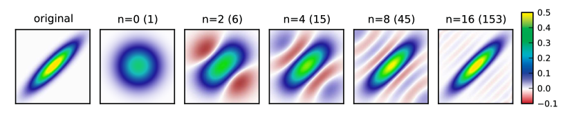
Figure 1: Circular shapelet approximations of increasing order $n$ to an elliptical Gaussian with an axis ratio of $1/4$. The number of basis functions ($\frac{1}{2}(n+1)(n+2)$) used in each approximation is given in parenthesis. Because the number of basis functions increases so dramatically at high order, the order of the expansion must be kept low for computationally feasible techniques, but low-order expansions produce distorted representations of even simple high-ellipticity morphologies.

A better solution, proposed by Nakajima & Bernstein (2007) (hereafter NB07), is to use elliptical basis functions to model the galaxy. To convolve with the PSF, one applies the inverse shapelet-space shear operator to the PSF to transform it into the coordinate system in which the galaxy is round. However, as the ellipticity of the galaxy model increases, the magnitude of the inverse shear transform that must be applied to the PSF model also increases, introducing approximation artifacts in the PSF model.

This trade-off is advantageous for two reasons. First, one can often afford to use a higher-order expansion for the PSF, because the PSF coefficients are not fully free parameters when fitting an individual galaxy; the PSF model is mostly determined separately using images of stars in the same field. In addition, when the galaxy radius is larger than the PSF, the undistorted galaxy model plays a larger role in determining the ellipticity of the convolved model than the now-distorted PSF model. Still, this technique does not eliminate the “shear artifact” ellipticity bias; it merely decreases it by substituting a distorted, approximate PSF model for a distorted, approximate galaxy model.

2 Radial Profiles

Shapelet expansions also have difficulty reproducing realistic galaxy radial profiles. The azimuthally averaged radial profile of a galaxy often follows a Sérsic law:

$$\mathrm{flux}\propto e^{-r^{1/n}}$$ (4)

with the Sérsic index $n$ generally greater than one. Disk galaxies typically have $n\approx 1$ (an exponential profile), while spheroidal galaxies often have $n\approx 4$ (the de Vaucouleurs profile) or greater. The shapelet expansion is based on the Gaussian function ($n=1/2$), and hence has a much softer core and sharper cutoff at large radii than a Sérsic profile with $n\geq 1$. In theory, the shapelet basis is complete, and can absorb these differences in higher-order terms, but in practice a finite shapelet expansion converges to a Sérsic model with high $n$ extremely slowly, producing a clear “ringing” pattern in the approximation. Figure 2 shows a typical case.

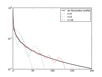
Figure 2: Shapelet approximations to a de Vaucouleurs (Sérsic $n=4$) profile. The radius and flux units are arbitrary, and the fit can be tuned to perform well at either small or moderate radii, but not both. Regardless of the scale of shapelet expansion, it will always fall off much faster at large radii compared to a pure de Vaucouleurs profile. This artificial truncation of the radial profile strongly affects flux and size estimates made using the model, and can bias the measured ellipticity as well, even when the truncation occurs at low surface brightness.

This poses a clear problem for the use of shapelets as a tool for morphological classification: the slope of the radial profile, arguably the clearest and most obvious distinction between galaxy types, is a nonlinear function of high-order terms in shapelet space. In contrast, it can be easily be estimated with a simple Sérsic fit or concentration measurement.

The inability to accurately reproduce realistic radial profiles also has implications for shear measurement. Ellipticity estimators based on model fitting have been shown to produce a multiplicative bias when the model is a systematically poor fit to the data (Voigt & Bridle, 2010; Bernstein, 2010). Using mock galaxies with Sérsic profiles, Melchior et al. (2010) have shown that this “underfitting bias” exists for shapelets even at relatively high orders. Even at low surface brightness, modeling the wings of galaxies properly can be very important in shear estimation, as the wings contain the low-spatial-frequency shape information that is corrupted least by convolution with the PSF (Bernstein, 2010).

A shapelet-like expansion based on general Sérsic profiles rather than Gaussians has been proposed as a possible solution to this problem (Ngan et al., 2009; Andrae et al., 2011), but these “Sérsiclets” lack many of the advantages of the shapelet basis, including analytic convolution and fast numerical evaluation, and thus far have not been used to construct a practical shear or morphological estimator.

3 Convolution of elliptical shapelets

In this section, we derive an exact analytic convolution formula for Gauss-Hermite functions. This provides the “missing ingredient” for making use of the elliptical shapelet basis of equation 2 to address the limitations of the standard shapelet basis at high ellipticity. This allows the PSF model and unconvolved galaxy model to be represented by elliptical shapelets with different basis ellipses, and determines an optimal basis ellipse for the convolved shapelet expansion that makes the convolution exact.

Consider a pair of functions and their convolution, each represented by a finite elliptical shapelet expansion in image coordinates:

$$f[\bm{x}] =\sum_{\bm{n}}^{|n|\leq N_{f}}f_{\bm{n}}\Phi_{\bm{n}}\!\left[\bm{U}^{-1}\bm{x}\right]$$ (5)

$$g[\bm{x}] =\sum_{\bm{n}}^{|n|\leq N_{g}}g_{\bm{n}}\Phi_{\bm{n}}\!\left[\bm{V}^{-1}\bm{x}\right]$$ (6)

$$(f*g)[\bm{x}] =\sum_{\bm{n}}^{|n|\leq N_{h}}h_{\bm{n}}\Phi_{\bm{n}}\!\left[\bm{W}^{-1}\bm{x}\right]$$ (7)

The boldface two-dimensional indices $\bm{n}$ each run over pairs of one-dimensional indices $\{n_{1},n_{2}\}$ as in equation 1, but for conciseness we will define the “magnitude” of a vector index as $|n|\equiv n_{1}+n_{2}$, as this combination will appear often.

The Fourier transforms of the circular shapelet basis functions are proportional to the basis functions themselves (Refregier, 2003), and the Fourier-space ellipse transform is simply the transpose of the inverse of the real-space ellipse transform, so

$$\tilde{f}[\bm{k}] =\left|\bm{U}\right|\!\sum_{\bm{n}}^{|n|\leq N_{f}}f_{\bm{n}}i^{|n|}\Phi_{\bm{n}}\!\left[\bm{U}^{T}\bm{k}\right]$$ (8)

$$\tilde{g}[\bm{k}] =\left|V\right|\!\sum_{\bm{n}}^{|n|\leq N_{g}}g_{\bm{n}}i^{|n|}\Phi_{\bm{n}}\!\left[\bm{V}^{T}\bm{k}\right]$$ (9)

$$2\pi\tilde{f}[\bm{k}]\,\tilde{g}[\bm{k}] =\left|\bm{W}\right|\!\sum_{\bm{n}}^{|n|\leq N_{h}}h_{\bm{n}}i^{|n|}\Phi_{\bm{n}}\!\left[\bm{W}^{T}\bm{k}\right]$$ (10)

$$=2\pi\left|\bm{U}\right|\left|\bm{V}\right|\!\sum_{\bm{p}}^{|p|\leq N_{f}}\sum_{\bm{q}}^{|q|\leq N_{g}}i^{|p|+|q|}\Phi_{\bm{p}}\!\left[\bm{U}^{T}\bm{k}\right]\Phi_{\bm{q}}\!\left[\bm{V}^{T}\bm{k}\right]$$ (11)

We can use the orthogonality of the basis functions to isolate the coefficients of the convolved expansion by multiplying by $\Phi_{\bm{m}}\!\left[\bm{W}^{T}\bm{k}\right]$ and integrating

$$h_{\bm{n}} =2\pi\left|\bm{U}\right|\left|\bm{V}\right|\!\sum_{\bm{p}}^{|p|\leq N_{f}}\sum_{\bm{q}}^{|q|\leq N_{g}}i^{|p|+|q|-|n|}\int\!d^{2}\bm{k}\,\Phi_{\bm{p}}\!\left[\bm{U}^{T}\bm{k}\right]\Phi_{\bm{q}}\!\left[\bm{V}^{T}\bm{k}\right]\Phi_{\bm{n}}\!\left[\bm{W}^{T}\bm{k}\right]$$ (12)

$$=2\pi\left|U\right|\left|V\right|\!\sum_{\bm{p}}^{|p|\leq N_{f}}\sum_{\bm{q}}^{|q|\leq N_{g}}i^{|p|+|q|-|n|}\;I_{\bm{p},\bm{q},\bm{n}}\!\left[\bm{U},\bm{V},\bm{W}\right]$$ (13)

To obtain the model convolution tensor $\bm{C}$ at pixel coordinates $\{\bm{x}_{j}\}$, we simply remove the sums over $\bm{p}$ and $\bm{q}$, and evaluate the expansion

$$C_{j,\bm{p},\bm{q}}=2\pi\left|\bm{U}\right|\left|\bm{V}\right|\sum_{\bm{n}}^{|n|\leq N_{h}}\Phi_{\bm{n}}[\bm{W}^{T}\bm{x}_{j}]\;i^{|p|+|q|-|n|}\;I_{\bm{p},\bm{q},\bm{n}}\!\left[\bm{U},\bm{V},\bm{W}\right]$$ (14)

To compute the integral, it is useful to separate the exponential and polynomial terms

$$I_{\bm{p},\bm{q},\bm{n}}\!\left[\bm{U},\bm{V},\bm{W}\right] =\int\!d^{2}\bm{k}\,\Phi_{\bm{p}}\!\left[\bm{U}^{T}\bm{k}\right]\Phi_{\bm{q}}\!\left[\bm{V}^{T}\bm{k}\right]\Phi_{\bm{n}}\!\left[\bm{W}^{T}\bm{k}\right]$$ (15)

$$=\int\!d^{2}\bm{k}\,e^{-\frac{1}{2}\bm{k}^{T}\left(\bm{U}\bm{U}^{T}+\bm{V}\bm{V}^{T}+\bm{W}\bm{W}^{T}\right)\bm{k}}\;Z_{\bm{p}}\!\left[\bm{U}^{T}\bm{k}\right]Z_{\bm{q}}\!\left[\bm{V}^{T}\bm{k}\right]Z_{\bm{n}}\!\left[\bm{W}^{T}\bm{k}\right]$$ (16)

with

$$Z_{\bm{p}}\!\left[\bm{U}^{T}\bm{k}\right] \equiv\mathcal{H}_{p_{1}}\!\left[U_{11}x_{1}+U_{21}x_{2}\right]\,\mathcal{H}_{p_{2}}\!\left[U_{12}x_{1}+U_{22}x_{2}\right]$$ (17)

$$\mathcal{H}_{n}\!\left[x\right] \equiv\left(\sqrt{\pi}\,2^{n}\,n!\right)^{-1/2}H_{n}\!\left[x\right]$$ (18)

We prefer the “normalized” Hermite polynomials $\mathcal{H}_{n}$ here over the standard Hermite polynomials $H_{n}$ both because they provide a more concise notation and because their recurrence relations (see Appendix 8.A) are more numerically stable (Press et al., 2002).

Returning to equation 16, we can simplify the exponential factor by requiring

$$\bm{W}\bm{W}^{T}=\bm{U}\bm{U}^{T}+\bm{V}\bm{V}^{T}$$ (19)

This reduces to the familiar formula for the convolution of elliptical Gaussians at zeroth order; for an elliptical shapelet expansion with ellipse transform $\bm{S}$, $\bm{S}\bm{S}^{T}$ is the covariance matrix of the Gaussian. We then make the substitution $\bm{W}^{T}\bm{k}\rightarrow\bm{y}$:

$$I_{\bm{p},\bm{q},\bm{n}}\!\left[\bm{U},\bm{V},\bm{W}\right] =\int\!d^{2}\bm{k}\,e^{-\bm{k}^{T}\bm{W}\bm{W}^{T}\bm{k}}\;Z_{\bm{p}}\!\left[\bm{U}^{T}\bm{k}\right]Z_{\bm{q}}\!\left[\bm{V}^{T}\bm{k}\right]Z_{\bm{n}}\!\left[\bm{W}^{T}\bm{k}\right]$$ (20)

$$=\frac{1}{|W|}\int\!d^{2}\bm{y}\,e^{-\bm{y}^{T}\bm{y}}\;Z_{\bm{p}}\!\left[\bm{U}^{T}\bm{W}^{-T}\bm{y}\right]Z_{\bm{q}}\!\left[\bm{V}^{T}\bm{W}^{-T}\bm{y}\right]Z_{\bm{n}}\!\left[\bm{y}\right]$$ (21)

Each normalized Hermite polynomial can be represented as a linear combination of monomials:

$$\mathcal{H}_{n}[x]=\sum_{m}^{N}M_{n,m}x^{m}\;,$$ (22)

where $M$ is the lower-triangular matrix of normalized Hermite polynomial coefficients. We can also write a monomial as a linear combination of normalized Hermite polynomials using the inverse matrix:

$$x^{m}=\sum_{n}^{N}M^{-1}_{m,n}\mathcal{H}_{n}[x]\;.$$ (23)

Along with the binomial theorem, these can be used to factor the ellipse-transform elements out of the polynomials:

$$Z_{\bm{n}}\!\left[\bm{T}\bm{x}\right] =\mathcal{H}_{n_{1}}\!\left[T_{11}x_{1}+T_{12}x_{2}\right]\,\mathcal{H}_{n_{2}}\!\left[T_{21}x_{1}+T_{22}x_{2}\right]$$ (24)

$$=\sum_{m1}^{N}\sum_{m2}^{N-m_{1}}M_{n_{1},m_{1}}M_{n_{2},m_{2}}\left(T_{11}x_{1}+T_{12}x_{2}\right)^{m_{1}}\,\left(T_{21}x_{1}+T_{22}x_{2}\right)^{m_{2}}$$ (25)

$$=\sum_{m1}^{N}\sum_{m2}^{N-m_{1}}\sum_{k_{1}}^{m_{1}}\sum_{k_{2}}^{m_{2}}\biggl{(}M_{n_{1},m_{1}}M_{n_{2},m_{2}}\,T_{11}^{m_{1}-k_{1}}\,T_{12}^{k_{1}}\,T_{21}^{m_{2}-k_{2}}T_{22}^{k_{2}}\,\biggr{.}$$

$$\quad\quad\quad\biggl{.}\times\;\binom{m_{1}}{k_{1}}\binom{m_{2}}{k_{2}}\,x_{1}^{m_{1}+m_{2}-k_{1}-k_{2}}\,x_{2}^{k_{1}+k_{2}}\biggr{)}$$ (26)

$$=\sum_{m1}^{N}\sum_{m2}^{N-m_{1}}\sum_{k_{1}}^{m_{1}}\sum_{k_{2}}^{m_{2}}\sum_{j_{1}}^{N}\sum_{j_{2}}^{N-j_{1}}\biggl{(}M_{n_{1},m_{1}}M_{n_{2},m_{2}}M^{-1}_{m_{1}+m_{2}-k_{1}-k_{2},j_{1}}M^{-1}_{k_{1}+k_{2},j_{2}}\biggr{.}$$

$$\quad\quad\quad\biggl{.}\times\;\binom{m_{1}}{k_{1}}\binom{m_{2}}{k_{2}}T_{11}^{m_{1}-k_{1}}\,T_{12}^{k_{1}}\,T_{21}^{m_{2}-k_{2}}\,T_{22}^{k_{2}}\,\biggr{)}\mathcal{H}_{j_{1}}\![x_{1}]\,\mathcal{H}_{j_{2}}\![x_{2}]$$ (27)

$$=\sum_{\bm{j}}^{|j|\leq N}Q_{\bm{n},\bm{j}}\!\left(\bm{T}\right)Z_{\bm{j}}\!\left(\bm{x}\right)$$ (28)

Plugging equation 28 into equation 21, we have

$$I_{\bm{p},\bm{q},\bm{n}}\!\left[\bm{U},\bm{V},\bm{W}\right] =\frac{1}{|W|}\sum_{\bm{l}}^{|l|\leq N_{f}}\sum_{\bm{m}}^{|m|\leq N_{g}}Q_{\bm{p},\bm{l}}\!\left[\sqrt{2}\bm{U}^{T}\bm{W}^{-T}\right]Q_{\bm{q},\bm{m}}\!\left[\sqrt{2}\bm{V}^{T}\bm{W}^{-T}\right]$$

$$\quad\quad\times\quad\int\!d^{2}\bm{y}\,e^{-\bm{y}^{T}\bm{y}}\;Z_{\bm{l}}\!\left[\bm{y}/\sqrt{2}\right]Z_{\bm{m}}\!\left[\bm{y}/\sqrt{2}\right]Z_{\bm{n}}\!\left[\bm{y}\right]$$ (29)

$$=\frac{1}{|W|}\sum_{\bm{l}}^{|l|\leq N_{f}}\sum_{\bm{m}}^{|m|\leq N_{g}}Q_{\bm{p},\bm{l}}\!\left[\sqrt{2}\bm{U}^{T}\bm{W}^{-T}\right]Q_{\bm{q},\bm{m}}\!\left[\sqrt{2}\bm{V}^{T}\bm{W}^{-T}\right]$$

$$\quad\quad\times\quad\int\!d^{2}\bm{y}\,\Phi_{\bm{l}}\!\left[\bm{y}/\sqrt{2}\right]\Phi_{\bm{m}}\!\left[\bm{y}/\sqrt{2}\right]\Phi_{\bm{n}}\!\left[\bm{y}\right]$$ (30)

$$=\frac{2}{|W|}\sum_{\bm{l}}^{|l|\leq N_{f}}\sum_{\bm{m}}^{|m|\leq N_{g}}Q_{\bm{p},\bm{l}}\!\left[\sqrt{2}\bm{U}^{T}\bm{W}^{-T}\right]Q_{\bm{q},\bm{m}}\!\left[\sqrt{2}\bm{V}^{T}\bm{W}^{-T}\right]$$

$$\quad\quad\times\quad B_{l_{1},m_{1},n_{1}}\!\left[\sqrt{2},\sqrt{2},1\right]\;B_{l_{2},m_{2},n_{2}}\!\left[\sqrt{2},\sqrt{2},1\right]$$ (31)

where $B_{l,m,n}$ is the one-dimensional triple product integral defined by Refregier & Bacon (2003); it can be computed directly with recurrence relations (see Appendix 8.B). The complete formula for convolution of elliptical shapelets is thus

$$h_{\bm{n}} =\frac{4\pi\left|U\right|\left|V\right|}{\left|W\right|}\!\sum_{\bm{p}}^{|p|\leq N_{f}}\sum_{\bm{q}}^{|q|\leq N_{g}}\sum_{\bm{l}}^{|l|\leq N_{f}}\sum_{\bm{m}}^{|m|\leq N_{g}}i^{|p|+|q|-|n|}\;Q_{\bm{p},\bm{l}}\!\left[\sqrt{2}\bm{U}^{T}\bm{W}^{-T}\right]Q_{\bm{q},\bm{m}}\!\left[\sqrt{2}\bm{V}^{T}\bm{W}^{-T}\right]$$

$$\quad\quad\times\quad B_{l_{1},m_{1},n_{1}}\!\left[\sqrt{2},\sqrt{2},1\right]\;B_{l_{2},m_{2},n_{2}}\!\left[\sqrt{2},\sqrt{2},1\right]$$ (32)

and the model convolution tensor is

$$C_{j,\bm{p},\bm{q}} =\frac{4\pi\left|U\right|\left|V\right|}{\left|W\right|}\!\sum_{\bm{n}}^{|n|\leq N_{h}}\sum_{\bm{l}}^{|l|\leq N_{f}}\sum_{\bm{m}}^{|m|\leq N_{g}}i^{|p|+|q|-|n|}\;Q_{\bm{p},\bm{l}}\!\left[\sqrt{2}\bm{U}^{T}\bm{W}^{-T}\right]Q_{\bm{q},\bm{m}}\!\left[\sqrt{2}\bm{V}^{T}\bm{W}^{-T}\right]$$

$$\quad\quad\times\quad B_{l_{1},m_{1},n_{1}}\!\left[\sqrt{2},\sqrt{2},1\right]\;B_{l_{2},m_{2},n_{2}}\!\left[\sqrt{2},\sqrt{2},1\right]\;\Phi_{\bm{n}}[\bm{W}^{T}\bm{x}_{j}]$$ (33)

Because $B_{l,m,n}\!\left[\sqrt{2},\sqrt{2},1\right]$ is zero for $n>l+m$, these relations are exact if $N_{h}\geq N_{f}+N_{g}$ and $W$ is chosen as the solution to equation equation 19, allowing an elliptical shapelet galaxy model to be convolved with an elliptical shapelet PSF model without approximation.

4 Modeling with Compound Shapelets

In this section we propose a simple solution to the radial profile problem: instead of increasing the order of a shapelet expansion in order to fit Sérsic-like profiles, we create a compound shapelet expansion that combines multiple low-order shapelet expansions with different radii. By adding a low-order expansion with small radius, a compound basis can represent a realistically cuspy core. Likewise, additional expansions with large radii should be able to compactly represent extended wings without introducing oscillatory artifacts.

In particular, we will consider compound basis functions of the form

$$\Psi_{n}\!\left[\bm{x}\right]=\sum_{j}^{j\leq N_{\beta}}\sum_{k}^{k\leq N^{(j)}_{\Phi}}M^{(j)}_{k,n}\,\Phi_{k}\!\left[\bm{x}/s_{j}\right]$$ (34)

The compound basis is thus composed of several shapelet bases, each with a different relative scale $s_{j}$. Each compound basis function may be a linear combination of several shapelet basis functions, with weights given by the matrices $\bm{M}^{(j)}$. When an ellipse transform is applied, the same transform is applied to all of the shapelet basis functions that comprise the compound basis. A compound basis is thus defined by a sequence of weight matrices $\bm{M}^{(j)}$ and relative scales $s_{j}$ (note that all the weight matrices will have the same number of columns, but may have differing numbers of rows).

1 Properties of the Compound Basis

Two notable properties of the standard shapelet basis are its orthonormality and completeness. Both of these are in general broken in the construction of a compound basis. The orthonormality condition for standard shapelets,

$$\int\!d\bm{x}\,\Phi_{\bm{j}}[x]\,\Phi_{\bm{k}}[x]=\delta_{\bm{j},\bm{k}}\;,$$ (35)

is defined for a continuous integral with infinite limits. While this is an important property for deriving analytic formulae involving shapelet basis functions, it is of limited practical use in decomposing image data into shapelets, because the pixelization and finite limits of image data do not match the idealized orthonormality condition; even standard shapelet basis functions are not orthonormal when projected to images (Massey et al., 2004). As a result, most standard shapelet decomposition techniques use linear least-squares methods that do not require orthonormality of the basis functions. In deriving analytic formulae (such as the convolution relation) for the compound basis functions, it is simpler to start with the analogous formulae for standard shapelets and multiply by the weight matrices $\bm{M}^{(j)}$ than to attempt to derive these from scratch on a new orthonormal basis.

However, the inner-stage importance function derived in section 4 does assume that a reasonable coefficient vector will have elements that are all within a few orders of magnitude, and a normalized basis will make this much more likely. We can orthonormalize an arbitrary basis by computing the actual matrix of inner products $\bm{P}$ for an arbitrary compound basis:

$$P_{m,n} \equiv\int\!d\bm{x}\,\Psi_{m}[x]\,\Psi_{n}[x]$$ (36)

$$=\sum_{i}^{i\leq N_{\beta}}\sum_{j}^{j\leq N^{(i)}_{\Phi}}\sum_{k}^{k\leq N_{\beta}}\sum_{l}^{l\leq N^{(k)}_{\Phi}}M^{(i)}_{j,m}\,M^{(k)}_{l,n}\int\!d\bm{x}\,\Phi_{j}\!\left[\bm{x}/s_{i}\right]\,\Phi_{l}\!\left[\bm{x}/s_{k}\right]$$ (37)

A diagonal $\bm{P}$ corresponds to an orthogonal basis, and $\bm{P}=\bm{I}$ corresponds to an orthonormal basis. The integral in equation 37 can be computed using recurrence relations (see Appendix 8.C). We can then modify the basis by multiplying the mapping matrices $\bm{M}$ by the inverse of a square root of $\bm{P}$. For instance, we can use the Cholesky factorization (where $\bm{L}$ is lower-triangular):

$$\bm{L}\bm{L}^{T}=\bm{P}$$ (38)

$$\bm{M}^{(j)}\rightarrow\bm{M}^{(j)}\bm{L}^{-1}$$ (39)

The new inner product matrix $\bm{P}$ is then the identity matrix by construction.

The formal completeness of the standard shapelet basis is also rarely useful in practice; while an infinite shapelet expansion can perfectly represent any function in $\mathbb{R}^{2}$, in practice we must work with finite expansions. As we have noted, a finite-size shapelet basis can be poor at representing the particular functions – those that mimic galaxy and PSF profiles – we are most interested in. While the finite-size compound basis thus lacks the completeness properties of the infinite standard shapelet basis, our essential argument is that a compound basis can be significantly more complete than a similarly-sized standard shapelet basis over the domain of functions we are most interested in.

2 Ellipse Degeneracies

While we have made a point of avoiding shapelet-space geometric transformation operators because they are not exact at finite shapelet order, the fact that they exist implies that the parameters $\bm{\phi}$ that enter through the ellipse transform will be highly degenerate with those linear combinations of basis coefficients $\bm{\alpha}$ that produce shapelet-space translation, shear, and scaling transforms. For a compound basis composed of low-order shapelet expansions, these degeneracies are reduced, because the basis functions poorly approximate the ellipse transform. However, even first- or second-order shapelet components will generally make the model too flexible, as first-order terms approximate a centroid shift, and second-order terms approximate changes in ellipticity and size.

Bernstein & Jarvis (2002) propose determining their equivalent of the ellipse parameters using a “null test” algorithm, in which the $\bm{\phi}$ parameters are iterated until the resulting expansion has zero centroid, zero ellipticity, and unit size in the ellipse-transformed coordinate system. This is equivalent to the linear constraint

$$\sum_{n}K_{m,n}\alpha_{n} =0$$ (40)

with

$$K_{1,n} =\int d^{2}\bm{\theta}\,\theta_{1}\,\Phi_{n}\![\bm{\theta}] K_{2,n} =\int d^{2}\bm{\theta}\,\theta_{2}\,\Phi_{n}\![\bm{\theta}]$$

$$K_{3,n} =\int d^{2}\bm{\theta}\,(\theta_{1}^{2}-\theta_{2}^{2})\,\Phi_{n}\![\bm{\theta}] K_{4,n} =\int d^{2}\bm{\theta}\,\theta_{1}\theta_{2}\,\Phi_{n}\![\bm{\theta}]$$

$$K_{5,n} =\int d^{2}\bm{\theta}\,(\theta_{1}^{2}+\theta_{2}^{2}-1)\,\Phi_{n}\![\bm{\theta}]$$ (41)

These can generally be computed using recurrence relations.

We can construct the analogous constraint matrix for a compound shapelet basis simply by replacing $\Phi$ with $\Psi$ above. Rather than applying the constraint when fitting individual galaxies, however, we can instead “circularize” the basis itself by modifying the weight matrices $\bm{M}$ in equation equation 34. Given a set of input basis functions $\Psi_{n}(\bm{\theta})$ and its constraint matrix $\bm{K}$, we first compute the singular value decomposition of $\bm{K}^{T}$:

$$\bm{U}\bm{D}\bm{V}^{T}=\bm{K}^{T}\;.$$ (42)

The diagonal matrix $\bm{D}$ will have at most five non-zero elements, corresponding to the first five columns of $\bm{U}$. The remaining columns of $\bm{U}$ give the mapping from the original basis to the circularized basis:

$$\Psi^{c}_{n}(\bm{\theta})=\sum_{m}\Phi_{m}(\bm{\theta})\;U_{m,n+5}$$ (43)

or

$$M^{c}_{k,n}=\sum_{m}M_{k,m}\;U_{m,n+5}\;.$$ (44)

The resulting basis is naturally five elements smaller than the input basis, and its constraint matrix is the zero matrix, so equation 40 is always true.

While a “circularized” basis may be useful when using a greedy optimizer to maximize the likelihood or posterior, ellipse degeneracies in a basis are actually desirable in our Monte Carlo algorithm. Because we can change the centroid, radius, or ellipticity of the model without changing the ellipse transform parameters, when we evaluate the model at a single ellipse point $\bm{\phi}$, we can actually represent a range of “effective” ellipses with variation in $\bm{\alpha}$. This allows us to more sparsely sample $\bm{\phi}$-space, as $\bm{\phi}$ points that are not sampled can be approximated by different combinations of $\bm{\alpha}$ parameters at nearby sample points. We can make this even more effective by ensuring that the ellipse derivatives of any particularly important basis functions can be represented as a linear combination of other basis functions – this allows the basis to function as a Taylor series in the ellipse parameters, and better approximate the “in-between” $\bm{\phi}$ points.

Allowing the ellipse degeneracies to remain in the basis clearly means any measurement of an ellipse quantity depends on the coefficients $\bm{\alpha}$, as well as the ellipse parameters $\bm{\phi}$. Unlike the flux measurement operator, these measurement operators are not linear in the coefficients. We can measure the effective ellipse by measuring the first and second moments of the model; the first moment vector is the centroid, and the second moment matrix can be related to the ellipticity and radius by the relations given in Appendix 7. These moments can be related to a set of linear operation vectors $\bm{e}_{i}$ that can be computed directly from the basis functions (similar to the rows of the constraint matrix $\bm{K}$), and are transformed by the inverse of the ellipse transform matrix $\bm{T}[\bm{\phi}]$. The first and second moment operators are:

$$\left[\begin{array}[]{c}I_{x}\\ I_{y}\end{array}\right] =\frac{1}{\bm{e}_{0}^{T}\bm{\alpha}}\bm{T}[\bm{\phi}]\left[\begin{array}[]{c}\bm{e}^{T}_{x}\bm{\alpha}\\ \bm{e}^{T}_{y}\bm{\alpha}\end{array}\right]+\hat{\bm{\theta}}[\bm{\phi}]$$ (49)

$$\left[\begin{array}[]{c c}I_{xx}&I_{xy}\\ I_{xy}&I_{yy}\end{array}\right] =\frac{1}{\bm{e}_{0}^{T}\bm{\alpha}}\bm{T}[\bm{\phi}]\left[\begin{array}[]{c c }\bm{e}^{T}_{xx}\bm{\alpha}-(\bm{e}^{T}_{x}\bm{\alpha})^{2}&\bm{e}^{T}_{xy}\bm{\alpha}-(\bm{e}^{T}_{x}\bm{\alpha})(\bm{e}^{T}_{y}\bm{\alpha})\\ \bm{e}^{T}_{xy}\bm{\alpha}-(\bm{e}^{T}_{x}\bm{\alpha})(\bm{e}^{T}_{y}\bm{\alpha})&\bm{e}^{T}_{yy}\bm{\alpha}-(\bm{e}^{T}_{y}\bm{\alpha})^{2}\end{array}\right]\bm{T}[\bm{\phi}]^{T}$$ (54)

with

$$(e_{0})_{n} =\int\!d^{2}\bm{\theta}\,\Psi_{n}\![\bm{\theta}] (e_{x})_{n} =\int\!d^{2}\bm{\theta}\,\theta_{1}\,\Psi_{n}\![\bm{\theta}]$$

$$(e_{y})_{n} =\int\!d^{2}\bm{\theta}\,\theta_{2}\,\Psi_{n}\![\bm{\theta}] (e_{xx})_{n} =\int\!d^{2}\bm{\theta}\,\theta_{1}^{2}\,\Psi_{n}\![\bm{\theta}]$$

$$(e_{yy})_{n} =\int\!d^{2}\bm{\theta}\,\theta_{2}^{2}\,\Psi_{n}\![\bm{\theta}] (e_{xy})_{n} =\int\!d^{2}\bm{\theta}\,\theta_{1}\theta_{2}\,\Psi_{n}\![\bm{\theta}]$$ (55)

We will return to the question of measuring ellipse parameters when we discuss shear estimation applications in section 3; it may be necessary to take additional steps to avoid systematic biases at extremely low levels.

3 Radii and Shapelet Order

The primary disadvantage of the compound basis technique is its flexibility. The user must select in advance the scales $s_{j}$ and shapelet orders $N^{(j)}_{\Phi}$ to be used in fitting an ensemble of galaxy images. This will typically require some experimentation on a smaller training sample of galaxies.

It is not immediately clear what metric to optimize in selecting the scales and shapelet orders, even for an ideal training set; one does not want to simply ensure the compound basis fits the mean morphology well. A better choice would be to optimize the full posterior of of all galaxies in the training sample, treating the individual galaxy parameters as nuisance parameters. This is a huge global nonlinear optimization problem, however, requiring each galaxy in the sample to be fit for a new ellipticity and set of coefficients for every iteration in the basis parameters. Furthermore, this metric imposes a signal-to-noise weighting on the members of the training sample, which may or may not be appropriate for different training sets. Most importantly, it is clear that a basis with a large total number of basis functions will generally outperform a basis with fewer, and thus part of the challenge is in determining the correct number of basis functions to use. There are also computational advantages to using fewer shapelet expansions, just as there are advantages in decreasing the order of the shapelet components, and a useful metric must assign weights to each of these opposing priorities.

One approach is to set the scales and shapelet orders to match a particular analytic function, such as an exponential or other fixed-index Sérsic profile. However, to do so, one must choose a metric that defines similarity between the analytic profile and its shapelet approximation. While a compound basis can approximate a Sérsic function over a wider range of scales than a standard shapelet basis, it still cannot reproduce a general Sérsic profile over the full infinite range of the function, and a metric that puts significant weight at large or very small radii typically produces a poor approximation over the range of radii where galaxy profiles can realistically be observed. These problems can be greatly mitigated by matching the basis to an apodized Sérsic function, which is modified to decrease rapidly to zero beyond some multiple of the half-light radius. Such apodized functions are common even when fitting pure Sérsic functions, reflecting the fact that we generally do not have any useful data beyond 4-5 half-light radii. Compound basis fits to apodized exponential ($n=1$) and de Vaucouleurs ($n=4$) profiles are shown in Figures 3 and 4. We can combine a few such profile-trained basis functions to form a basis with similar flexibility to a full Sérsic fit with variable $n$; we can then add terms with higher-order shapelet functions to support more complex morphologies.

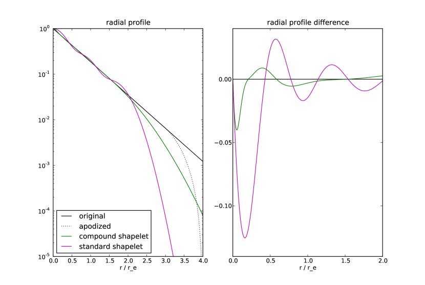
Figure 3: Standard and compound shapelet fits to a modified exponential (Sérsic $n=1$) profile, where the modification is a polynomial truncation at $r_{e}=4$ (the same prescription as used in the SDSS galaxy modeling). The standard shapelet approximation is 8th order, while the compound shapelet fit uses only 4 zeroth-order (Gaussian) profiles. The panel on the right shows the difference between the original Sérsic profile and the shapelet approximation at small radius.

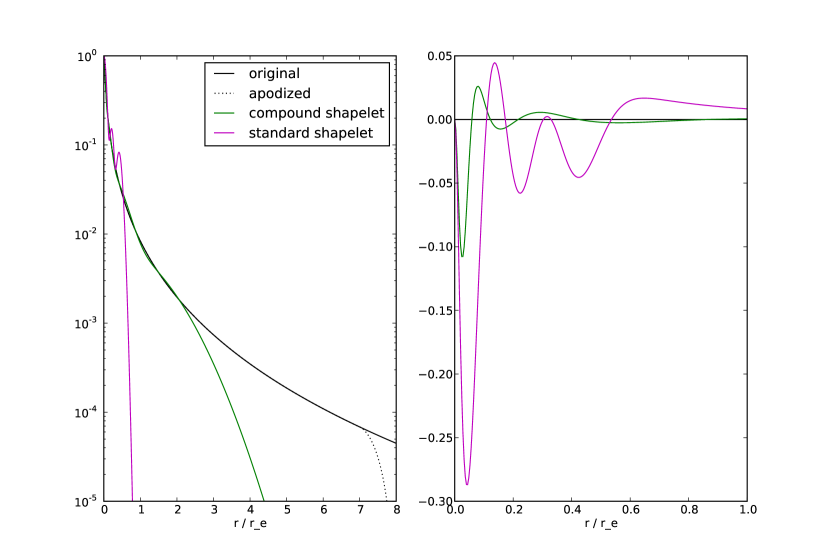
Figure 4: Standard and compound shapelet fits to a modified de Vaucouleurs (Sérsic $n=4$) profile, where the modification is a polynomial truncation at $r_{e}=8$ (the same prescription as used in the SDSS galaxy modeling). As in Figure 3, the standard shapelet approximation is 8th order, while the compound shapelet fit uses only 4 zeroth-order (Gaussian) profiles (but the relative scales of the Gaussians is different from Figure 3). Note that the difference panel on the right uses a different radius range than that of Figure 3. While even the compound shapelet approximation truncates much earlier than the original profile, it does a good job in the region we are likely to have data.

4 Dimensionality Reduction

Because the radii and shapelet orders must be chosen in advance, a compound basis will typically have a fixed number of elements, and unlike the standard shapelet basis, there is no consistent way to increase or decrease the size of the basis to match the signal-to-noise ratio (S/N) and resolution of the image data being modeled.

Given a training sample, one can attempt to mitigate some of these problems by changing the weight matrices $\bm{M}$, eliminating those linear combinations of basis functions which do not play an important role in fitting the training sample. This can be used to produce a “reduced” compound basis, in which the number of basis functions can be much smaller than the number of shapelet basis functions used to build it. Quantifying the “importance” of a basis function is difficult, however, and may vary between different modeling applications and datasets.

In spite of this, we expect some sort of dimensionality reduction to be a crucial part of any computationally feasible weak-lensing or morphological analysis technique based on compound shapelets, and we will explore this more fully in a future paper. It may also be an important step in using the training sample to determine the optimal scales and shapelet orders of the component expansions; while we have discussed the two problems separately here, constructing a basis from a training sample involves optimizing $s_{j}$, $N^{(j)}_{\Phi}$, and $\bm{M}^{(j)}$ together.

5 Priors and Linear Constraints

The problem of building a basis from a training sample is also closely linked to the problem of building an empirical coefficient prior to go with it. In an ideal sense, the problem is to characterize the intrinsic distribution of galaxy morphologies, using an arbitrary linear basis; we then wish to project to a new basis that somehow simplifies that distribution. The standard method for basis selection, principal components analysis (PCA), would treat this distribution as Gaussian, and identify the most important basis functions as the directions with the largest variance. We can imagine extending this to a mixture-of-Gaussians clustering approach that could handle multimodal distributions. As we have noted, a Gaussian or mixture of Gaussians is not appropriate as a coefficient prior on its own, as it does not account for the steep slope of the prior as a function of flux. We may be able to use a Gaussian or Gaussian mixture distribution in the normalized coefficients (i.e. $\tfrac{\alpha}{\lVert\alpha\rVert}$), however, and this would naturally work well with the importance distribution of equation 111.

The first roadblock to such efforts is the need to “bootstrap” the initial distribution using some other, non-optimal basis. We have had some success modeling simulated galaxies using a simple basis consisting of a few Sérsic profile approximations (such as those of Figures 3 and 4), along with a single second-order shapelet expansion to provide desirable ellipse degeneracies. To build a distribution from a training sample, however, we require a much more flexible basis, such as the combinations of higher-order shapelet functions listed in Table 1. A more flexible basis has greater need for an informative prior, however, unless the data quality is extremely good. We have sidestepped this in the next section by simply using a maximum-likelihood fit, which may also be an option in the bootstrap phase of building a basis and corresponding prior.

Even if we must start with a flat prior, however, we can make use of linear inequality constraints to reduce the volume of the space that prior includes, and reject unphysical models. We can view these constraints as part of the prior; they essentially define a polytope in parameter space, with the prior set to zero outside this region. Highly flexible compound shapelet models can suffer from severe extrapolation problems without such constraints, as a compound basis can easily have flexibility well beyond the maximum radius constrained by the data. These are easily addressed through positivity and monotonicity constraints, which can be written as linear inequality constraints on the coefficients (and do not depend on $\bm{\phi}$). To avoid removing too much flexibility, we can even define a smoothed monotonicity constraint, in which we require a smoothed radial profile to be monotonic. These constraint-based flat priors should be viewed as a temporary solution, however; the real goal is an empirical prior.

5 Demonstration and Results

To demonstrate the improvements that compound and elliptical shapelets offer relative to more standard shapelet techniques, we apply the compound shapelet models to the Frei et al. (1996) sample of nearby galaxies. This data set has high S/N and a very small PSF relative to the galaxy sizes, and spans a wide range of morphologies. Even though these conditions are not typical of most weak-lensing observations, this is an ideal data set for testing the suitability of our basis functions in fitting the true, unconvolved morphologies of galaxies, even with application to shear measurement. While the distribution of morphologies for the moderate- and high-redshift galaxies used in weak-lensing measurements is not identical to the distribution of morphologies in our sample, the same morphological types will be present in both, and a nearby galaxy sample affords relative image quality that is significantly better than even the best space-based or adaptive optics imaging of more distant galaxies.

$\beta$	0.25	0.50	1.00	2.00	4.00
__8__	-	-	8	-	-
_44_4	-	4	4	-	4
_444_	-	4	4	4	-
4_4_4	4	-	4	-	4
4_44_	4	-	4	4	-
206_3	2	0	6	-	3
2063_	2	0	6	3	-
026_3	0	2	6	-	3
0263_	0	2	6	3	-

Table 1: Shapelet order at five different radii for the nine demonstration basis sets.

Of the 113 galaxies in the sample, 82 were observed in $R$ and $B_{j}$, and the other 31 in $g$, $r$, and $i$. We limit our attention to the $B_{j}$ and $g$ images (the two filters are very similar). We fit each of the 113 galaxies in the sample with both the elliptical and circular forms of each basis described below, but discard the 31 galaxies in which the fit did not converge in one or more cases (these failures are mostly due to large gradients in the background present in some of the images).

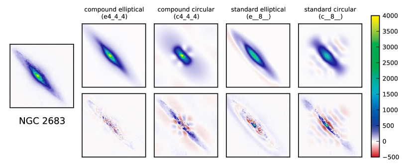
Figure 5: Image, shapelet models (upper), and residuals (lower) for NGC 2683, a typical edge-on spiral galaxy in our test sample. Each model has 45 free parameters, equivalent to an 8th-order standard circular shapelet fit. This example clearly illustrates the artifacts introduced in circular shapelet fits to high-ellipticity galaxy images; in this case, the circular models actually have negative flux in certain regions. As expected, the compound and standard shapelet fits perform similarly at moderate radii, but the compound basis is noticeably better at representing structure at small and large scales, modeling the core well while reducing or eliminating the “ringing” residuals present in the wings of the standard basis fits. The basis labels are defined in Table 1, and the data and fitting procedure are described in section 5.

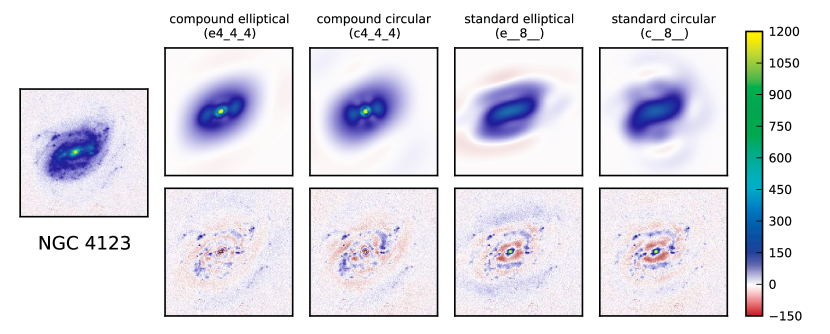
Figure 6: Image, circular shapelet models (upper), and residuals (lower) for NGC 4123, a typical face-on spiral galaxy in our test sample. The elliptical compound basis models the core, bar, and ring structure reasonably well, but none of the models capture much of the spiral arm structure. This is generally the case for the face-on spirals in our sample.

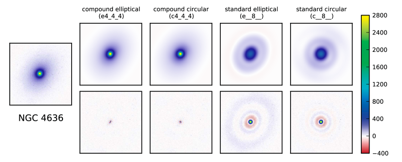
Figure 7: Image, shapelet models (upper), and residuals (lower) for NGC 4636, a typical massive elliptical galaxy in our test sample. The difference between the compound basis fits and the standard basis fits is striking, particularly in the oscillating residuals and in the core of the galaxy, which is not fit at all by the standard basis. Both circular fits show residuals which are clearly circular, rather than matched to the ellipticity of the galaxy, and the standard circular shapelet model is quite clearly circular at large radii, even though the galaxy is not; the limited basis simply does not have the modeling power to apply the correct shear at both moderate and large radii.

We consider nine compound basis sets, including a single-scale standard shapelet basis, each with 45 basis functions (before circularization). These are summarized in Table 1. For elliptical shapelet fits (e prefix), we circularize the basis and fit for the coefficients and ellipse parameters simultaneously using the Levenberg–Marquardt nonlinear least-squares optimizer. The initial ellipse parameters are determined from the unweighted moments of the image. For circular shapelet fits (c prefix), we fix the centroid and size to the results from the elliptical fit, and perform a linear least-squares fit using the uncircularized basis. In each case, there are 45 free parameters. We use a simple circular Gaussian PSF model (with FWHM as given in the image headers).

1 Results

The results for three representative galaxies are shown in Figures 5, 6, and 7. As expected, the edge-on spiral galaxy (Figure 5) demonstrates most clearly the improvement from circular to elliptical shapelets, both for the compound basis (4_4_4) and the standard basis (__8__). The difference can also be seen in the c__8__ fit to the elliptical galaxy (Figure 7). Because the standard shapelet expansion already has such difficulty representing the de Vaucouleurs profile, it cannot afford to “spend” coefficients on matching the ellipticity of the galaxy. The compound basis provides better fits to both the inner radii and outer radii of all the galaxies shown, and eliminates the “ringing” residuals except at very small radii; this is particularly dramatic for NGC 4636. None of the basis sets provide enough flexibility to fit the spiral arms of NGC 4123 (Figure 6) well, and this is generally the case for the face-on spirals in the sample. The compound basis fits do provide a reasonably good approximation to the bar and ring structure, and all the fits do a moderately good job of fitting the overall profile of the spiral galaxies.

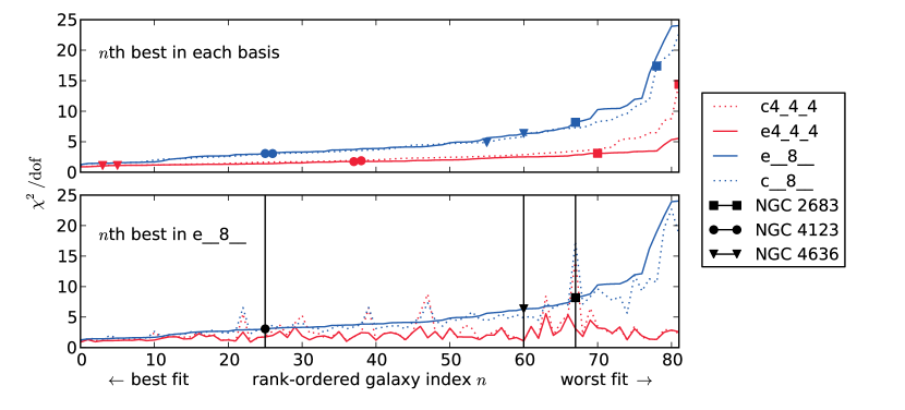
Figure 8: Rank-ordered goodness of fit for 82 galaxies from the Frei et al. (1996) sample of nearby galaxies, for selected elliptical and circular shapelet basis sets. In the upper plot, the galaxies are rank-ordered by reduced $\chi^{2}$ for each basis separately; each point on the $x$-axis thus corresponds to the $n$th best-fit galaxy for each basis. In the lower plot, the reduced $\chi^{2}$ from the e__8__ fit is used to set the galaxy rank index for all bases; a point on the $x$-axis thus corresponds uniquely to a single galaxy. The goodness of fit for the galaxies shown in Figures 5, 6, and 7 are given by the square, circle, and triangle points, respectively. The circular standard basis actually produces slightly lower average and worst-case residuals than the elliptical standard basis, but the compound elliptical basis is significantly better than either. The high-ellipticity edge-on spirals (such as NGC 2683) that present a particular problem for the circular shapelet expansion can be clearly seen in the lower plot as spikes in the circular basis goodness-of-fit.

These tendencies are quantified in Figure 8, which shows the goodness-of-fit distribution for the 82 galaxies successfully fit with all basis sets. The elliptical compound basis consistently has the lowest residuals, and even the circular compound basis generally outperforms both the elliptical and circular standard shapelet basis. The elliptical standard shapelet basis is not uniformly better than the circular standard shapelet basis, but the cases where it is – high-ellipticity edge-on spirals, like NGC 2683 – stand out clearly as spikes in the lower plot, in which the galaxy index is consistent across all the fits. It is also worth noting that when the compound basis is used, featureless, low-ellipticity early-type galaxies like NGC 4636 have some of the lowest residuals in the sample. In contrast, these have moderately large residuals compared to the rest of the sample for the standard shapelet basis fits, demonstrating that using a compound basis essentially solves the problem of fitting de Vaucouleurs profiles with shapelets, at least from a goodness-of-fit standpoint.

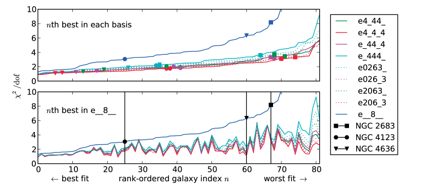
Figure 9: Goodness-of-fit comparison for all elliptical basis sets. The rank-ordered indexing and galaxy sample are the same as in Figure 8, but the $y$-axis scale has been changed to show more detail. All of the compound shapelet basis sets outperform the standard shapelet basis for all galaxies but one, in which the results are comparable, and the compound bases show considerably better worst-case performance. Between compound basis sets, those with components at both the largest and smallest radii (4_4_4 and 206_3) consistently have the lowest residuals.

Figure 9 similarly shows the distribution goodness-of-fit for all elliptical basis sets. The most obvious result is that all the compound shapelet bases tested outperform the standard shapelet basis, both in aggregate and (with one slight exception) for every galaxy individually. Between the compound basis sets, those with shapelet expansions at both $\beta=0.25$ and $\beta=4.0$ tend to perform slightly better, especially compared to basis sets that contain neither, suggesting that compound bases are most effective when constructed with shapelet orders at radii that differ by more than a factor of two. This provides a partial answer to the question of how to choose the radii and orders of the component shapelet bases that is both frustrating and somewhat comforting: while there is no clear choice for an optimal combination of radii and orders, any reasonable choice that samples the radial range of significant morphology is still a marked improvement over the standard shapelet basis.

6 Summary and Future Work

Despite the problems discussed in section 2, shapelets have become one of the most important tools in galaxy modeling, particularly in weak lensing. The inability of the standard shapelet basis to represent morphologies with high ellipticity or steep profiles puts limits on the accuracy of shapelet-based shear estimators, however, and likely degrades the performance of shapelet-based morphological analyses. We have presented here two techniques to address these limitations.

The first is a convolution relation for elliptical shapelets. This eliminates the need to use the lossy shapelet-space shear operator, and allows ellipse-parameterized shapelets to be used in place of a circular basis parameterized only by centroid and radius. While the elliptical basis requires five nonlinear parameters to be fit instead of three, the two additional parameters more than pull their weight in modeling power, particularly for high-ellipticity galaxies. Perhaps most importantly, an exact elliptical shapelet convolution allows shapelet-based shear estimators to be constructed that do not suffer from the “shear artifact” bias discussed in section 1. The results of section 5 do not demonstrate the advantages of the elliptical convolution formula; while we used it in fitting the galaxies, the size of our test galaxies relative to the PSF makes the difference between our exact convolution and the approximation of NB07 negligible. However, this formula can be immediately put to use in existing elliptical shapelet shear–measurement methods, such as that of NB07, eliminating one source of bias for galaxies near the resolution limit.

To address the difficulties of the standard shapelet basis in fitting galaxies with high Sérsic indices, we have introduced the concept of a “compound” shapelet basis – a basis composed of multiple low-order shapelet expansions with different scale radii. Even with simple, ad-hoc choices for the radii and orders of the component shapelet expansions, the compound basis is significantly better than a single higher-order shapelet expansion at fitting realistic galaxy morphologies, particularly in its worst-case performance. By combining low-order shapelet basis functions at multiple radii, a compound basis can compactly represent both the sharp cores and extended wings of galaxies with high Sérsic indices. As we have seen, this can make a significant difference even in spiral galaxies with relatively low Sérsic indices, and almost completely eliminates the oscillatory artifacts often present in standard shapelet fits. This should reduce the underfitting shear bias for shapelet-modeling shear measurement methods, but whether the bias can be reduced to acceptable levels for future surveys is a question we reserve for a future paper. Morphological analyses such as those of Kelly & McKay (2004) and Andrae et al. (2010) should also benefit from utilizing compound shapelet basis sets, as the more compact compound shapelet representation essentially gives classification and clustering algorithms a head start in reducing the dimensionality of the problem.

Unlike the elliptical convolution formula, further work is needed to make full use of the compound shapelet concept in a complete shear measurement or morphological analysis method. While we have demonstrated success in fitting nearby galaxies with unoptimized basis sets and a simple fitting algorithm, more challenging modeling problems may require techniques that tune the parameters and weights of a compound basis using a training sample of galaxies. Such a basis of “eigenmorphologies”, built from analytically tractable shapelet building blocks, would be an extremely powerful tool, not only for morphological analysis, but also in further quantifying and reducing underfitting biases in model-based shear measurement techniques.

Chapter 3 Applications

1 Photometry

Measuring the fluxes and colors of astronomical objects using the methods we have developed is fairly straightforward. The total flux of the model is a simple linear operator on the coefficients $\bm{\alpha}$:

flux $$=\int\!d\bm{\theta}g[\bm{\theta},\bm{\phi},\bm{\alpha}]$$ (1)

$$=\int\!d\bm{\theta}\sum_{i=1}^{N}\tilde{\Psi}_{i}[\bm{\theta},\bm{\phi}]\alpha_{i}$$ (2)

$$=\sum_{i=1}^{N}\alpha_{i}\bigl{|}\bm{T}[\bm{\phi}]\bigr{|}\int\!d\bm{\theta}\Psi_{i}\!\left[\bm{T}[\bm{\phi}]^{-1}(\bm{\theta}-\hat{\bm{\theta}}[\bm{\phi}])\right]$$ (3)

$$=\sum_{i=1}^{N}\alpha_{i}\int\!d\bm{\theta}^{\prime}\Psi_{i}\!\left[\bm{\theta}^{\prime}\right]$$ (4)

$$=\bm{v}^{T}\bm{\alpha}$$ (5)

$$v_{i} \equiv\int\!d\bm{\theta}^{\prime}\Psi_{i}[\bm{\theta}^{\prime}]$$ (6)

Because the model is multiplied by the determinant of of the ellipse transform $\bm{T}$, we can change variables to remove the dependence on $\bm{\phi}$, and as a result the flux operator $\bm{v}$ does not depend on the ellipse parameters. The weighted sample $\{\bm{v}^{T}\bm{\alpha}_{[n,m]},w_{[n,m]}\}$ is thus representative of the posterior distribution of the flux. Similarly, we can apply a logarithm transform to our sample to obtain the posterior distribution of the magnitude.

This has some clear advantages over the more common procedure of estimating “best-fit” fluxes with symmetric variance-based error bars. While the magnitude system does not permit negative fluxes, “best-fit” fluxes can be negative (and their lower bounds based on symmetric error bars are very often negative). These do not transform easily to the magnitude system, necessitating the development of alternate definitions such as the hyperbolic arcsin magnitudes used by the SDSS (Lupton et al., 1999), and making the transformation of uncertainties to regular magnitudes somewhat problematic. While arcsinh magnitudes have other advantages, it is worth noting that the negative flux problem is limited to non-Bayesian techniques. Any reasonable prior will assign zero probability to a model with an unphysically negative flux, and this will naturally carry over to the posterior. This may present some problems in terms of publishing (asymmetric) confidence limits in public catalogs, but it is clearly a better reflection of reality.

The photometric measurements produced by our Monte Carlo sampling approach also differ from standard photometric measurements in that they cannot easily be related to an aperture magnitude. Most maximum likelihood modeling methods for measuring flux can be seen in some sense as an aperture method by viewing the profile of the model as a continuous aperture; while the slope and radius of the profile model may be allowed to vary, the flux is measured with these fixed at their maximum-likelihood values. With our approach, the flux is marginalized over the other parameters of the model, so the effective profile is the posterior-weighted average of the profile at all the Monte Carlo sample points. This provides a much more complete and robust accounting of the uncertainties involved in measuring the flux, but it may also make it difficult to compare our measurements with historical measurements, or more importantly, to calibrate our measurements to a standardized magnitude system. This should be viewed as a challenge, not a disadvantage; we should not a reject careful and robust treatment of uncertainties to make our results match up with expectations.

This challenge is perhaps most evident in the question of how to measure galaxy colors. Because of the intrinsic difficulty in measuring the absolute magnitude of a galaxy, quality estimates of flux ratios across different filters (colors) are generally more important. Historically galaxy colors have been measuring by applying the same aperture (or equivalently, a model with all parameters but amplitude fixed) to data from each filter. We do not have a single set of parameters to “fix” a model at in our paradigm, however. The closest approximation would be to run our algorithm on one canonical band, and use the exact same Monte-Carlo points in other bands, allowing only the amplitude of the model to vary and changing the weights accordingly. Real galaxies have different morphologies at different wavelengths, however, producing color gradients that inevitably make the choice of aperture a factor in the measured color. There is no “magic” aperture or model that produces correct colors; the real reason we use the same aperture or model in different bands is simply because it ensures consistency. Measuring colors with maximum likelihood modeling techniques that allow the profile parameters to vary across different bands lacks this needed consistency simply because the modeling technique is not robust – fluxes are not marginalized over uncertainties in the profile parameters, and can change significantly when the best-fit profile parameters are perturbed by noise. With our more robust modeling methods, this consistency should be easier to achieve, but it is still crucial to require the models to be similar in different bands, simply because the S/N may be extremely low in some bands and large in others due to the spectrum of the object. This can be achieved by fitting to all filters simultaneously, and allowing the object to have different linear parameters $\bm{\alpha}$ on different filters but the same nonlinear parameters $\bm{\phi}$. We can then use the prior on the linear parameters to ensure that the colors are reasonable and the morphologies in different filters are similar.

We can use a similar approach when fitting variable objects, using a single set of nonlinear parameters and a different set of linear parameters for each exposure. Most variable astronomical objects are point sources, so this results in only one linear parameter per exposure. For point sources, the nonlinear parameters will generally model stellar motions, rather than the ellipse of an extended object; sharing those parameters across exposures allows us to construct models for variable stars with proper motion and parallax. Just as with fitting galaxies to multiple bands, we can define a coefficient prior for the variable point source model that will ensure the variability levels are physically reasonable.

In some cases, we may wish to use more complex models that connect these multiple observations in place of a simple prior. When modeling galaxies, for instance, we could evaluate the posterior of a photometric redshift model in place of the coefficient prior. This would entail adding additional nonlinear parameters to account for the redshift and spectrum of the object, which must be explored in the outer stage. In the inner stage, we would evaluate the posterior of the photometric redshift model using the fluxes defined by the linear coefficients as the data. Similarly, we could fit a light curve model directly to the pixel values when modeling variable objects, rather than allow the fluxes to vary independently on different exposures. These proposals may be significantly more computationally expensive than the methods used today, but they would provide better measurements for the faintest objects, as well as a more robust accounting of uncertainties. The question of how much better is an open one, however, and it is likely that we could obtain similar results just by making use of the full flux posteriors when modeling redshifted galaxy spectra or light curves, even if we do not apply them directly to the pixels.

Finally, we should note that almost all of these methods require the final photometric calibration to be in place before the modeling algorithms are run. The photometric calibration sets the weights of individual exposures, and these are combined with the rest of the inputs in a complex way by the modeling algorithm. For the case of galaxy modeling, in which a single set of linear parameters are shared across multiple exposures, there is no way to correct the outputs of the algorithm for changes in the photometric calibration without recomputing all the Monte Carlo weights (which would require reevaluating the model at all of the nonlinear parameter points). For variable objects, the situation is slightly better, as we can identify a single set of linear parameters that correspond to each exposure. This breaks down if we make use of scientifically interesting priors on the variability, or simultaneously fit nonvariable and variable objects. While we could use a different set of linear parameters for each exposures even for nonvariable objects, this would entail a significant increase in the degrees of freedom of the model and would thus make any measurements based on the model much noisier, especially in the short-exposure limit.

2 Astrometry

We have already mentioned the possibility of including proper motion and parallax among the nonlinear parameters when fitting stars to multiple exposures simultaneously. This approach has already been demonstrated with a non-Monte Carlo modeling method by Lang et al. (2009). It is particularly valuable for stars that are too faint to appear in individual exposures, a regime where both coadd-based approaches and single-exposure modeling are completely inadequate; while we may still rely on the coadd for detection, we cannot measure motion there, and we cannot even measure centroids on individual exposures. This does present some problems for our adaptive importance sampling algorithm; unlike the galaxy models, we cannot adapt our importance distribution to an approximate coadd-based posterior before switching to more expensive multi-exposure modeling. This could require more iterations of importance sampling, or perhaps initialization with a greedy optimizer. Point source models are significantly faster to evaluate than PSF-convolved galaxy models, however, so this may not be impractical, even at large scales.

3 Shear Estimation

Weak gravitational lensing is one of the most important – and most demanding – applications of large multi-epoch surveys. Our goal here is limited to measuring an unbiased ellipticity for each lensing source galaxy. A lack of bias is by far the most important requirement; the lensing shear is a small fraction of the observed ellipticity of a typical galaxy, so we must spatially average the ellipticities of thousands of galaxies to obtain a measurable lensing signal. Any spatially correlated or constant bias in the ellipticity measurement will thus be amplified many times, potentially dwarfing the lensing effect, especially in the extremely weak regime of lensing by large-scale structure. The PSF is the main source of difficulties in weak lensing measurements; the spatial variation in the ellipticity of the PSF can easily mimic a physical shear signal. Furthermore, even convolution by an isotropic PSF will modify the observed ellipticity, usually decreasing it.

Simply using a forward-fitting modeling technique (in which we convolve the model with the PSF) corrects for both of these problems, assuming the PSF model is adequate. Basing the ellipticity measurement on an imperfect model introduces its own systematic effects, however, and some of these are exacerbated by the PSF convolution. The most obvious are underfitting biases, in which the model is not flexible enough to match the data. These do not fit easily into the standard picture of ellipticity measurement as a process that depends only on low-order morphological information, and hence can be performed on faint and barely-resolved galaxies. One of the reasons modeling biases are difficult to address is that higher-order morphological information in the model is transferred to lower spatial frequencies by the PSF convolution, making the observable ellipticity dependent on aspects of the model that are naturally hard to constrain from the data.

We have already discussed underfitting problems with standard shapelet models in Chapter 2, and demonstrated that they can be greatly mitigated by using multi-scale elliptical shapelets. When a model is flexible enough to represent realistic galaxy profiles, however, it is likely it will often be under-constrained by the likelihood, and the prior may have a significant effect on the result. This is an improvement over the underfitting problem, however, as long as we marginalize our ellipticity measurements over the other parameters in the model, and make use of the full resulting ellipticity distribution. Most ellipticity measurement algorithms do not marginalize, however, and most weak lensing techniques do not even make use of any uncertainty estimate for the ellipticities of individual galaxies, let alone the full distribution. This likely accounts for some of the success of the shear estimation method of Miller et al. (2007), which does make use of the full ellipticity distribution. This cannot fully account for the fact that some aspects of our model are unconstrained by the data, however, and the prior will necessarily impact the measurement. We can choose a prior that reduces any biases we measure in simulations, but this is little better than the current practice of applying an empirically-determined “fudge-factor” to our measurements, as it is still subject to differences between our simulated distribution of morphologies and the real distribution.

Bernstein (2010) approaches this problem from another perspective. We can add a weight function to the ellipticity measurement operators defined in section 2, and define this measurement in Fourier space, as an operator that acts on the Fourier transform of the model. Because convolving the model with the PSF destroys high spatial frequency features of the model, we can define a Fourier-space weight function that ignores these high spatial frequency features and hence does not depend on features of the model that have been censored by the PSF. The practical implementation proposed by Bernstein (2010) involves using a standard shapelet decomposition to generate a Fourier-space representation of the data that the Fourier-space weight function can be applied to. As a result, the method is still subject to some of the limitations of the shapelet basis in representing real galaxies that we discuss in section 2. The final problem with this method is that it creates a different definition of ellipticity for each galaxy, as the weight function depends on the relative sizes of the galaxy and the PSF. This complicates the procedure of estimating the shear from a catalog of ellipticity measurements, because the meaning of each measurement – and hence its sensitivity to the lensing effect – is slightly different.

Our compound-shapelet galaxy models can also be easily Fourier-transformed, and should represent a much better way to generate the Fourier-space realization needed by the modified weight function. Moreover, by applying this ellipticity measurement to our full Monte Carlo sample of parameter vectors, we can more correctly account for the full uncertainty distribution of the ellipticity, and hence address model biases that are not strictly due to the convolution; these will generally be much less severe than those imposed by the convolution, but they should not be ignored entirely. This may also allow us to relax the truncation of the ellipticity weight function at large spatial frequency, which would make the definition of the ellipticity for different galaxies more similar.

With this general approach, a number of other features of our modeling method provide additional advantages for weak lensing measurements. First, by marginalizing over the centroid parameters of the model, we can eliminate the “centroid bias” that allows PSF spatial variation to print through to ellipticity measurements in a subtle way (Kaiser, 2000). Essentially, an elongation in the PSF in one direction increases the noise in the centroid in that same direction; meanwhile, an error in the centroid produces an error in the estimated ellipticity if the centroid is held fixed rather than marginalized.

By fitting multiple objects simultaneously, we can also reduce the effects of neighboring objects on shear measurements. While we may not be able to obtain usable measurements from severely blended objects, we should be able to reduce any small biases that result from slight overlaps. This should be particularly important for cluster and galaxy-galaxy lensing, in which source galaxies close to the line of sight of the center of the mass distribution are of course more likely to be at least partially obscured by foreground galaxies associated with that mass distribution.

Finally, we should note that making full use of many of the ideas in this section will require a fundamental change in how we view “higher-level” weak lensing measurements. Current methods typically make use of catalogs of ellipticities; future methods should be prepared to deal with catalogs of ellipticity distributions, with the added complication that these ellipticities may each have a slightly different definition. Some weak lensing studies already make use of Bayesian methods, and may be easy to adapt to these different ellipticity measurements. Others – the 2-point functions (and higher-order statistics) commonly used in cosmic shear studies in particular – may be harder to adapt.

4 Morphology and Classification

The flexibility of our galaxy model is also important for studies of galaxy morphologies. While morphological studies of based on poorly-resolved or low S/N galaxies are always difficult, a generative modeling approach at least has the potential to avoid strong systematic effects due to the PSF and low surface brightness. Many popular automated morphological estimators (Abraham et al., 1994; Bershady et al., 2000; Lotz et al., 2004) make use of direct statistics on the observed image, and such estimates are inherently biased by the image quality (as are morphological classifications based on visual inspection). Traditional methods thus almost always tend to find more complicated morphologies as data improves, and correcting for this known bias is a difficult problem. This may be true in the modeling case as well – we still lose high spatial frequency information due to the PSF, and our best-fit models may be systematically smoother and less cuspy as a result. Similarly, our model may lack low surface brightness features when these are buried in the noise – but by characterizing the full posterior and using a sufficiently flexible model we can at least “know how much we don’t know” in a robust sense; when the data is poor, we may not choose more complicated morphologies as the best fit, but we can establish when they cannot be ruled out. And as we have discussed, if we can train an informative prior on a small sample of higher-quality data, we can essentially make the right guesses when we are forced to consider the parts of the model we cannot constrain with the data.

A galaxy model with many linear parameters is a natural fit to a machine learning approach to morphological classification, and studies based on standard shapelets have already made some progress in this area (Kelly & McKay, 2004; Andrae et al., 2010). We believe these were limited by the use of a non-elliptical shapelet basis, as much of the variance in the measured shapelet coefficients was simply due to variations in ellipticity. As a result, both studies were able to easily distinguish edge-on and face-on spiral galaxies, and showed some ability to distinguish both from ellipticals, but could not go much further. Improving upon these efforts is central to the question of building an optimal basis and training an empirical prior on the basis coefficients. As we have discussed, such a basis and accompanying prior would have great potential for improving the models, but it is extremely challenging. The work so far on automated morphological classification using linear galaxy models is still in a “proof of concept” phase, limited to convenient, magnitude-limited datasets and the most basic properties of galaxies, but the stage is set for much more advanced work that makes use of larger, more representative samples, more flexible models, and a more robust accounting of modeling errors.

Robust modeling also has an important role to play in the much simpler question of how to distinguish stars from galaxies. Most Bayesian model selection methods make use of the evidence ratio of the two models (see, for example, chapter 4 of Sivia & Skilling 2006), which we naturally compute as part of our modeling algorithm. We can construct other estimators using other properties of the model as well, such as the half-light radius of the galaxy model, or by comparing the measured flux in both models. An important feature for any of these is our robust accounting of the model uncertainties; any naive classifier based on the PSF model that does not take into account its uncertainty will fail when that uncertainty is large, as will any classifier based on estimated galaxy size when we lack the ability to put rigorous confidence limits on the measured radii.

Finally, Bayesian modeling methods can play an important role in classifying objects that are actually “garbage”, or have significant data quality issues on one or more exposures. This is an important part of automated data quality assessment – we should not expect a perfect set of masks as input, especially when the evidence also provides a powerful way to indicate the goodness-of-fit and hence discover bad data. Unlike a high $\chi^{2}$, a low evidence does not merely indicate large residuals; it can also flag good fits with “unlikely” combinations of parameter values, indicated by a low overlap of the prior with the likelihood. This is also indicative of a problem with the data (or possibly a new class of astronomical object). While the evidence for a single object is difficult to interpret, we will fit many objects with similar brightness and size, and we can flag outliers in the evidence for additional inspection after binning along these axes.

5 Deblending

We have emphasized throughout that our modeling algorithm can be applied to multiple astronomical objects simultaneously. This is an important part of analyzing crowded fields, but it is not a complete solution by itself; we also require a way of generating a deblending hypothesis for how many objects are present, roughly where they are, and what types they may be. While our modeling technique may allow us to rigorously compare these hypotheses, it is easy to imagine even simple blends producing an unwieldy number of hypotheses. With just three objects and two types of models (variable point sources with proper motions and static galaxies, for instance), we would need to fit the system $2^{3}$ times to account for all possibilities. In addition, complex deblending models will have many more parameters than single-object models, making each system significantly more expensive. Happily, much of the additional expense will be in additional adaptive importance sampling iterations that should be performed on the coadd. Still, as survey depth increases, more objects will overlap, and it may be that most objects will be fit in pairs or triplets. It will become increasingly important to have a deblender that can generate good hypotheses and reject in advance highly unlikely permutations of object types, to reduce the number of deblending models that must be fit.

Additional computational expense aside, simultaneous modeling provides some significant scientific advantages for dealing with blended objects. The primary advantage is that our rigorous Monte Carlo characterization of the uncertainties allows us to marginalize over neighboring objects we do not care about, correcting measurements for the presence of undesirable foreground or background objects. When multiple objects in a blended set are of interest, the Monte Carlo samples correctly account for the correlations between their measured properties.

When fitting multiple exposures simultaneously, our models also allow us to take advantage of additional time domain information when assigning flux to different sources. The classic example in this case is strong gravitational lensing of quasars by galaxies. By fitting a static galaxy model simultaneously with a set of variable point-source models, we can better measure both the light curves of the quasars and the profile of the galaxy. If we marginalize over uncertainties in the PSF model rather than hold it fixed, we can even use this additional information to make up for deficiencies in the PSF model. We can also use this technique to deblend supernovae from their host galaxies, particularly if we put an informative prior on the light curve. Finally, if we fit multiple filters simultaneously, we can use a strong prior on the colors of objects to aid in deblending as well. While this may make it more difficult to find rare objects with extreme colors, it would provide an improvement in the photometry of most blended objects, and may represent the only way to attempt to separate severely blended objects.

The current state-of-the-art in deblenders, represented by the SDSS deblender (Lupton, 2005), operates entirely separately from the measurement process, assigning a fraction of each pixel’s flux to each object in such a way that all of the flux in each pixel is accounted for. Measurement algorithms, including modeling methods, then operate on these fractional pixel values, making it unnecessary to fit multiple objects simultaneously. Accounting for all the flux is clearly an attractive feature, and the pixelized, symmetry-based models used by the SDSS deblender are much more flexible than we expect our shapelet models to be. Unfortunately, generalizing these models to the multi-exposure case is difficult, and while they can still be used to generate a deblending hypothesis on the coadd, they cannot be used directly to divide per-pixel flux on individual exposures. While we may be able to develop a procedure to transform these sort of pixelized models to the individual exposures (by convolving them with the difference kernel between the coadd and each exposure, for instance), we argue that it will be better not to divide per-pixel fluxes before the modeling stage. Clearly simultaneous modeling provides much better control over the uncertainty; dividing the pixel fluxes essentially ignores uncertainty in deblending that may in fact be the dominant source of error in the measurements. The only way avoiding simultaneous modeling will produce better results – aside from performance questions, which admittedly may be a factor – is if the models used to divide pixel fluxes are a significantly better fit to the data than the measurement models, to the extent that the measurement models cannot be used to reconstruct most of the data. This is certainly possible if the measurement models are too simple, but this situation would also produce large modeling biases in our measurements even when deblending is not a factor, so we view improving the measurement models as the best solution to this problem.

6 Public Catalogs

All of our approaches to measurement have focused on characterizing the full posterior distribution of quantities by applying measurement operators to our Monte Carlo sample of parameter vectors. This is only possible while we actually have the Monte Carlo sample available, and thus requires that we know the desired measurements in advance (and can reduce their posterior distributions to a few descriptive numbers), or that we store the Monte Carlo sample and make it available as one of the data products of the survey.

Ignoring for a moment the question of whether the latter proposal is practical, consider the advantages:

• We do not need to realize nearly as many concrete measurements, making catalog database tables much “thinner”. Because we can efficiently compute most measurements on the fly, we do not need to anticipate all catalog-like measurements in advance.

• Users will be able to make use of the full posterior distribution of any measurement, including much higher-level measurements that are usually based on catalog entries for many objects, with full control over how to marginalize over other model parameters and neighboring objects.

• New operations that would have otherwise required access to the image data will be able to make of the model samples instead, potentially reducing the costs of image access and public compute resources.

• New data from outside sources can be correctly combined with the measurements, by using the same models and multiplying the posteriors.

Because the priors are shared and easily stored, this also allows users to use a slightly different prior, simply by multiplying the weights by the ratio of the new prior to the original one. As discussed by Hogg & Lang (2011), a probabilistic approach involving generative models, like this one, is simply the correct way to view the outputs of an astronomical survey; catalogs are at best convenient approximations.

Unfortunately, this approach may also be totally impractical – while we do not have good estimates of either the size of the Monte Carlo samples needed or the number of linear parameters, the uncompressed size of the samples could easily approach the size of the imaging data. Whether the samples could be compressed efficiently is an open question, however, and we can always reduce the sample size by extracting a random subsample. If we choose such a subsample by resampling with the weights, we will draw more points from the regions with higher probability, and possibly decrease the sample size without increasing the variance. And if making the samples available to the user does reduce direct image access, this change might be viewed as a trade-off between compute resources and storage resources.

Regardless, while providing direct access to the full modeling results is a challenging technical problem, and it represents a paradigm shift in how public surveys publish their data, it is almost certainly a positive paradigm shift, and the challenge should be viewed as one worth some technical effort.

Chapter 4 Implementation

1 Pipeline Overview

A complete discussion of the data flow and dependencies for a full survey reduction pipeline is beyond the scope of this paper, but it is worth spending some time to discuss how our measurement methods will interact with the rest of the pipeline. Figure 1 is a high-level diagram of the idealized data flow and dependencies. It includes several circular dependencies, reflecting the fact that reduction is an iterative process; measurements feed into self-calibration procedures that are used to improve the measurements. A practical pipeline diagram would involve decisions regarding which relationships to ignore, and which iterative procedures should loop until a condition is met and which should simply be performed a fixed number of times.

A few aspects of Figure 1 require some additional discussion and/or explanation. The numbers below refer to the numbers in the figure.

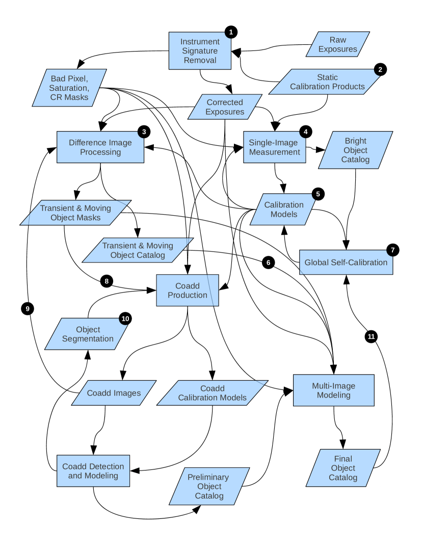
Figure 1: Idealized data reduction pipeline data flow and dependencies. Most processes and relationships are self-explanatory; numbered items are described in the text.

1. “Instrument Signature Removal” (a name taken from the LSST pipelines) refers simply to the basic image reduction operations that operate on entire images: de-bias, flat-field, fringe removal, etc. Here we also assume it includes cosmic ray and saturation detection.

2. “Static Calibration Products” are inputs to calibration models that do not depend on the pipeline outputs (or depend so weakly that they are updated on an entirely different schedule). These include detector correction images like bias frames, as well as global astrometric and photometric standard catalogs.

3. “Difference Image Processing” is a stage in which a coadd is convolved to match an individual exposure and subtracted from it, allowing transient, moving, and variable objects to be detected. This generates a catalog of objects (after the detections from each exposure are matched and reconciled). We can also build a mask to avoid including pixels affected by moving objects and transients in the coadd and during multifit.

4. In “Single-Image Measurement”, we detect and measure the properties of objects that are bright enough to appear in individual exposures, using only one exposure at a time. We also generate the first version of the calibration models for the PSF, background, astrometric solution and photometric solution.

5. By “Calibration Models”, we mean exactly those quantities we have included in our modeling algorithm as nuisance parameters: the PSF and background models for each exposure, as well as the relative astrometric and photometric calibrations. It is only the relative calibrations that participate in the dependency cycles; changes to the absolution calibration can be easily applied to the final catalogs with no need for iteration.

6. We do not limit multifit to just those objects that are detected on the coadd; we also want to include transient objects that are detected only in the difference images (and often deblend them from the static and slow-moving objects found on the coadd). Extremely fast-moving objects like asteroids can be fit in a multi-epoch sense as well, though this may present a challenge for organizing the image data efficiently.

7. In “Global Self-Calibration”, the relative astrometric and photometric models are improved by requiring measurement consistency across all overlapping sets of exposures (e.g. Padmanabhan et al. 2008). We also envision a global PSF modeling step such as the PCA approach developed by Jarvis & Jain (2004). All of these operations are formally global, as the entire survey must be tied together, but an implementation that operates on large subsets of the data may be sufficient for some iterations, as long as these are in agreement at the end. Unfortunately, global calibration steps may also introduce small inter-exposure covariance terms in the uncertainties of the calibrations, which would complicate slightly the marginalization algorithm in section 3.

8. When building a coadd, there are several options on how to handle time-domain information. One option is to use masks from the difference image processing to try to leave such objects out of the coadd entirely. We can also use an outlier rejection method to attempt to remove the objects without using masks. On the other hand, it may be useful to define the coadd as a strict mean that includes time-domain objects. Our tentative recommendation would be to build coadds that include variable and slow-moving objects (i.e. those that move less than a typical PSF over the course of the survey) in the coadd, while removing true transients and fast-moving objects. The best measurements for all faint time-domain objects will have to come from a multi-epoch modeling procedure, but a coadd defined this way will maximize the usefulness of the coadd in setting up those models. Using outlier rejection is an attractive possibility due to its lack of dependency on the difference imaging, but it makes the construction of a PSF model for the coadd much more difficult, as the effective weights of different exposures differ from pixel to pixel in a way that depends on the noise.

9. A coadd is a necessary ingredient in the sort of difference imaging we imagine (though it may be necessary to start by differencing pairs of individual exposures). The choices we discussed above in how to handle time-domain objects in the coadd have important implications for what difference image detections and measurements mean, and play a role in how deciding how best to resolve the circular relationship between coadds and difference images.

10. As we have discussed, an optimal coadd cannot have masked pixels, image edges, or a variable PSF within any pixel region that contains an astronomical object of interest. This means we should segment the sky based on the locations of objects, and “round-off” all defects and edges on individual exposures to the nearest segmentation boundary. This segmentation can only be built by detecting on a full-depth coadd, however, making at least two phases of coadd production necessary if coadd measurements need to be high-quality.

11. If we expect to use faint objects in our self-calibration procedures, the final self-calibration stage must occur after the multifit procedure. However, we cannot fully make use of improved calibration models without performing the multi-epoch modeling after the final self-calibration. This is one of the most difficult cycles to resolve. Ideally, we would be able to meet our self-calibration goals using only bright objects that are measured on individual exposures. If not, all the options are poor: we can either perform a second multifit step (faster than the first, since we only need to recompute the weights, but still expensive), or we can correct the measurements for the changes in the calibration at the end. This would require fitting different measurements on all exposures even for galaxy models, dramatically reducing the S/N of those measurements while dramatically increasing the size of the catalogs.

2 Scaling and Parallelization

Implementations of the algorithm and modeling procedures we have described are not yet mature enough for concrete performance measurements to be anything but misleading. However, it is useful to note briefly how the algorithm scales along certain axes, and discuss some of the options for parallelization.

First, it is worth noting that in the many-exposure limit, the number of pixels will be far larger than the number of linear or nonlinear parameters, even for small objects. It is thus very important that the worst-case complexity of the model in the number of pixels (and similarly, the number of exposures) is linear, except in the case of variable objects (in which the number of coefficients scales with the number of exposures). Happily, we expect to fit variable objects with simple point source models, so the computational expense involved in evaluating those models on each exposure is also considerably less. Since each set of coefficients only affects one exposure, the model matrix is also sparse in a block sense, and has exactly as many nonzero elements as the matrix for a nonvariable model. For galaxies, we expect the dominant computational expense to be evaluating the models on each exposure, even though we perform many operations with worse than linear complexity in the number of linear parameters for each model evaluation.

To evaluate a (compound) convolved shapelet model on a single exposure, we must evaluate the ellipse-transformed shapelet basis functions on each pixel; the order of the convolved basis is equal to the sum of the PSF order and the intrinsic galaxy model order, and the number of elements in the basis is proportional to the square of the convolved basis order. Reducing the order of the shapelet bases involved in modeling galaxies and PSFs is thus an important avenue for optimization; many low-order bases with different orders can easily outperform fewer high-order bases when convolution is involved. We expect the total number of basis functions to be between 10 and 50, so the size of these basis matrices also virtually ensures that the algorithm will be limited by memory or (most likely) CPU constraints, rather than I/O constraints. For each segmented region containing a single galaxy, we will need to evaluate perhaps 20-30 outer-stage Monte Carlo points; for each of these, we must evaluate a matrix with 10-50 times more elements than the number of data pixels.

Any modeling procedure for individual astronomical objects can easily be parallelized along the catalog axis; we simply assign each segmentation region to a different processor. While multi-object deblending segmentations will take longer, this parallelization requires virtually no communication between nodes. Our nested Monte Carlo procedure suggests two more fine-grained natural parallelization axes that may also prove useful. For a more traditional (e.g. multicore CPU) computing environment, parallelizing along outer-stage Monte Carlo points is an attractive option, requiring synchronization only when updating the outer-stage importance function. Each core would then be responsible for a single model matrix evaluation, as well as sampling from the corresponding inner-stage importance function. In a manycore (i.e. GPU) environment, we should parallelize along individual pixels when computing the model matrices; each exposure maps easily to a block of lightweight threads, and the shapelet recurrence relations are exactly the sort of math-heavy, single-instruction multiple-data operations that GPU processors excel at. The remainder of the operations are essentially dense linear algebra operations, and would also naturally translate extremely well to a manycore implementation.

Chapter 5 Related Work

We have already touched on several modeling methods that have features in common with the one we have developed here. In this chapter, we will discuss a few of these in detail, emphasizing the advantages and disadvantages of their approach relative to ours.

1 Shapelets and Sérsiclets

Gauss-Laguerre and Gauss-Hermite functions first started to see extensive use modeling galaxies following Bernstein & Jarvis (2002) and Refregier (2003). The latter coined the term “shapelets” to refer to both sets of basis functions, which have since been used in a variety of applications. Our approach is most similar to Nakajima & Bernstein (2007), who also transform the basis functions by transforming the input coordinates rather than using shapelet-space operators, and also convolve the model with the PSF before comparing it with data. Unlike a full generative model approach, however, their “forward fitting” algorithm iterates until a constraint similar to equation 40 is met, rather than maximizing the full likelihood or posterior. They also use an approximate convolution using shapelet shear operators, but the exact convolution relation we have derived in section 3 could easily be used instead in their algorithm and would likely improve the results.

The failure of shapelet models to fit realistic galaxy profiles has led to the proposal of similar basis sets based on general Sérsic profiles by Ngan et al. (2009) and Andrae et al. (2011), which they have called Sérsiclets. While they do provide much better fits to typical galaxies, these basis functions do not have many of the convenient properties of shapelets. In particular, they do not have an analytic convolution relation, making them inconvenient to use in generative models, which must be convolved efficiently with a PSF model. While building an approximate Sérsiclet basis using compound shapelet basis techniques may provide a way around that problem, the Sérsiclet basis functions do not provide any benefits beyond an empirically reasonable profile at zeroth order and an orthogonal set of higher-order functions; there is no reason to believe the first or second-order Sérsiclet basis functions are more useful than higher-order terms. We can much more easily obtain a compound shapelet basis with these properties simply by using the Cholesky orthogonalization method introduced in section 1.

2 Lensfit

The Lensfit code of Miller et al. (2007) and Kitching et al. (2008) was the first to apply Bayesian methods to the shear estimation problem. The success of this method, both with the GREAT08 simulations (Bridle et al., 2010) and the CFHTLS lensing survey, is one of the primary reasons we believe Bayesian methodology and a robust accounting of uncertainties based on generative models have an important role to play in shear estimation.

The Lensfit algorithm is different from ours in several respects, however. First, they sample the likelihood on a grid, rather than using Monte Carlo methods. This provides a more deterministic accounting of errors, but does not scale well to higher dimensions (i.e. large numbers of parameters). This has two important implications. First, the Lensfit models are relatively simple; they use a fixed Sérsic profile, and allow only the ellipse parameters to vary. These models are probably sufficient for most lensing source galaxies in terms of information content, but they may impose a small systematic modeling bias in the shear estimate; Voigt & Bridle (2010) have shown that Sérsic model biases are not negligible when fit with maximum-likelihood methods, and it is not clear whether this persists with the more sophisticated Bayesian modeling approach. Lensfit also makes use of a clever Fourier-space method to marginalize over the centroid automatically, which reduces the dimensionality of the grid.

This automatic marginalization may be problematic in the many-short-exposures limit, however. Lensfit combines data from multiple exposures by simply multiplying the likelihoods at each grid point. This means the centroid marginalization is carried out before combining the likelihoods, effectively considering the model to have a different centroid on each exposure. When each exposure has sufficient depth to effectively measure a centroid using data from that exposure alone, this increase in the number of degrees of freedom is relatively unimportant, and it may even help account for errors in the astrometry. When we have many short exposures, however, the centroid likelihood on an individual exposure is broad, and marginalizing over these broad distributions individually (instead of marginalizing over their much narrower product once) will produce a significant degradation in the ellipticity measurement.

3 Coadd-Based Shear Estimation

Prospects for effectively measuring ellipticities for weak-lensing on image coadds are not as bleak as they were once thought to be, thanks largely to a practical procedure for building a PSF model for the coadd due to Jee & Tyson (2011). Combined with a practical implementation of the Kaiser optimal coadd algorithm mentioned earlier, under certain conditions a coadd-based modeling method should be equivalent to a multi-exposure modeling method. None of these conditions will be exactly met in realistic conditions, but most will be nearly met most of the time:

• The PSF must not be spatially varying; in practice, this is almost always a safe approximation on the spatial scales of a single source galaxy image.

• No pixels must be masked out, and there must be no edges to images in the modeling region. In practice, this means we must discard images with bad pixels, cosmic ray hits, saturation, or image boundaries near an object of interest; this would then require a separate coadd for each object (or blended group of objects) to avoid throwing away too much data. We would suffer a small loss in signal-to-noise, and building these multiple coadds will be more expensive than a single coadd (because some overlap regions may be coadded many times). In contrast, with multi-exposure modeling we discard bad data pixel-by-pixel, instead of exposure-by-exposure.

• Image noise must be stationary. In practice, this means we must be in the sky-noise-dominated limit, which will generally be the case for most lensing source galaxies, but will not be true for brighter foreground galaxies and stars that may be nearby.

• Calibration models must have negligible uncertainties. While we cannot say that correctly marginalizing over calibration uncertainties is impossible with a coadd-based approach, no method for doing so exists, so at present we must require that calibration models be well-determined enough that their uncertainties do not contribute significantly to the total error budget.

Because coadd-based methods cannot be used at all for variable or moving objects, multi-exposure methods should also be considered necessary when deblending galaxies from possibly variable or moving stars.

These stringent requirements, along with the fact that we must use multi-exposure methods when fitting stars, may suggest that we should simply avoid coadd-based procedures. But fitting on a coadd – even the per-object coadds discussed above – can be orders of magnitude faster than fitting to multiple exposures, especially if most of the computation time is spent evaluating and convolving the model. We have already discussed the importance of using a coadd for most iterations of our adaptive importance sampling algorithm, in which we do as little work as possible in “multifit mode”. In the same vein, we should consider the possibility that for some objects all of the above conditions will be met satisfactorily, and we may not need a final multifit step. We should thus view the coadd generation process as an important one, and our goal should be the best possible coadd-based measurement (rather than simply a “quick and dirty” measurement needed to bootstrap a lengthy multifit procedure). Even if we can only rarely skip the multifit step, doing so is a powerful optimization. If we cannot skip the multifit step, better characterization of the importance distribution on the coadd will still allow us to save time in the multifit stage.

Chapter 6 Conclusion and Future Work

The methodology we have described in this paper is essentially an ambitious proposal to change how we build astronomical catalogs from photometric survey data. In the ideal case, it is even a proposal to change what we consider “catalog” to mean. It is also, necessarily, an incomplete proposal. The core of this work – the Monte Carlo algorithm described in Chapter 1, and the shapelet-based approach to build and convolve galaxy models in Chapter 2 – constitutes a full prescription for a method to robustly model galaxies. But testing and iterative improvement is a necessary part of making any method practical, and we have proposed many other ideas that require significant further development.

Perhaps the most important piece is simply the idea of a Bayesian approach to survey data reduction. We are not the first to advocate this approach, but very little work has been done to make the idea practical. There are two important aspects of a Bayesian approach. First, we should rigorously characterize the actual distribution of uncertainties on measurements, including correlations between measurements. This does not mean we must avoid, for instance, Fisher matrix methods – but we must validate such approximations. Second, we should consider uncertainties in calibration models, and include them in our measurements, ideally through marginalization. This is the crucial step in moving from generative models for individual astronomical objects to a single self-consistent generative model for an entire survey. In both cases, the crucial point is not that approximations are to be avoided – the concern is that when we do not take these steps, we tend to systematically underestimate uncertainties. Most real-world distributions have broader tails than Gaussians, and marginalization of a nuisance parameter rarely tightens a constraint.

When we cannot approximate some distributions with Gaussians, or ignore the impact of calibration parameters on our measurements, data reduction is almost inevitably more computationally expensive. We cannot rely on Moore’s Law and the rapid improvement in hardware capabilities, however – these same forces drive the increase in astronomical data volumes, and we must instead look to algorithmic improvements. Moreover, these complex algorithms are more important from a science standpoint as data volumes grow, as the increase in sample sizes leads to a decrease in stochastic sources of error, which makes understanding and addressing systematic errors more important.

The nested Monte Carlo importance sampling algorithm we have developed provides an example of both the challenge and the sort of algorithmic research needed. Even with a highly-optimized implementation, it will almost certainly be slower than an optimized version of most modeling methods commonly used today, but it does much more, marginalizing over calibration parameters and supporting an extremely flexible and general class of models, all while making very few assumptions about the behavior of the likelihood or prior distributions. By using a linear model and taking advantage of the near-Gaussianity of the marginal likelihood, we can draw many Monte Carlo points for each model evaluation, decreasing the number of expensive multi-exposure model evaluations needed to produce reasonable estimates.

It remains to be seen whether a compound shapelet approach will be the most effective way to provide convolvable models for this algorithm and others like it. Shapelet methods seem well positioned with regard to certain trends in hardware architectures (namely GPU-based computing), in which a simple, highly-parallelizable brute-force method may be more efficient than a more complex and memory-intensive lookup-table approach, but such trends are difficult to predict, and of course actual performance tests will have to decide. The shapelet convolution relation and “compound basis” techniques we have developed provide simple solutions to the biggest drawbacks of current shapelet methods, but the compound shapelet approach in particular could benefit greatly from further study. While we can construct usable compound shapelet models from combinations of Sérsic-profile components, and fit these with the flat, linear-constraint priors we have described, the method has a great deal more potential with an empirically-trained basis and informative prior.

This is where perhaps the most scientifically interesting future work is needed. Current efforts to characterize galaxy morphologies using linear basis functions have focused almost exclusively on shapelets and shapelet-inspired bases so far, and have been limited by the flexibility of those models and, frankly, the extreme difficulty of the problem. PCA and machine-learning methods have been powerful in similar classification and dimensionality reduction problems in other areas of astronomy and cosmology, however, and our ellipse-transformed galaxy models and robust handling of the PSF may provide the necessary boost to make these approaches more useful in quantifying galaxy morphologies. This is an interesting topic in its own right, but it also provides a way to take advantage of both narrow space-based surveys and wider ground-based surveys. By training a galaxy basis and a prior on higher-resolution space-based data, we can better infer the properties of much larger samples of galaxies observed from the ground.

Tying these galaxy modeling methods into a larger pipeline must also be the subject of a great deal of future work. We cannot make use of algorithms that handle calibration uncertainties unless those uncertainties are themselves well-characterized. This is in some respects a more difficult challenge than modeling galaxy morphologies; calibration models must essentially be able to model all the myriad ways the optical system can (mis)behave, or at least provide a way to reject data from modes that cannot be modeled. We must also deal with the fact that many of the steps in a survey pipeline have intrinsically circular dependencies, including the measurement and calibration modeling stages; these must be resolved by a carefully study of the implications of changes in ordering and the number of iterations. Finally, we should put serious effort into addressing the challenge of making a full characterization of the generative models for astronomical objects available to the public. We have proposed doing this by making the actual Monte Carlo samples and weights our algorithm produces the actual “catalog” users see (along with indices for searching and filtering some common measurements, of course). This may not be necessary, and it may not be the most efficient way to accomplish this goal – but the information we do make available in catalog form should be equivalent in terms of information content, or at least represent a conservative rather than optimistic characterization of the uncertainties. While this may be more expensive than standard catalog access, it allows us to provide support for Bayesian analyses without requiring users to access the raw pixel data.

The topics addressed in these thesis have often been at the boundary of astronomy, and have considerable overlap with more “methodological” fields such as computer science, applied mathematics, and statistics. These topics are extremely important for astronomy, however, and must be addressed at least in part by astronomers and physicists. They also must be addressed in advance; many of the ideas in this thesis are most applicable to the LSST, which is nearly a decade away from operation, though they will also be applied to smaller surveys in the interim. Yet this is likely scarcely enough time for some of these ideas to be fully realized, requiring us to work on simulation data or precursor surveys that have already been mined for their most important results. Efforts to improve data reduction algorithms – and build practical software implementations of them – are an integral part of building a public survey facility, and while they may sometimes seem removed from the high-level science questions that drive the fields of astronomy and astrophysics as a whole, they is no less important to the march of scientific progress.

Appendices

Chapter 7 Ellipse Parameterizations

Ellipses are widely used in astronomy to represent the shapes of extended objects, and can be parameterized in a number of ways, usually involving exactly five numbers. Almost all of these use a center coordinate point to indicate the position, leaving three numbers to define the ellipticity, radius, and orientation of the ellipse. The most familiar form uses the semimajor axis $a$, the semiminor axis $b$, and the position angle $\varphi$ (we will measure $\varphi$ as the angle from the $x$-axis to the major axis).

Another common form, which we will call the “quadrupole” or “moments” representation with parameters $\{q_{xx},q_{yy},q_{xy}\}$, is more easily related to the moments of a function $f[x,y]$:

$$q_{0} \equiv\int\!dx\,dy\,f[x,y]$$ (1)

$$q_{x} \equiv\frac{1}{q_{0}}\int\!dx\,dy\,x\,f[x,y]$$ (2)

$$q_{y} \equiv\frac{1}{q_{0}}\int\!dx\,dy\,y\,f[x,y]$$ (3)

$$q_{xx} \equiv\frac{1}{q_{0}}\int\!dx\,dy\,(x-q_{x})^{2}\,f[x,y]$$ (4)

$$q_{yy} \equiv\frac{1}{q_{0}}\int\!dx\,dy\,(y-q_{y})^{2}\,f[x,y]$$ (5)

$$q_{xy} \equiv\frac{1}{q_{0}}\int\!dx\,dy\,(x-q_{x})(y-q_{y})\,f[x,y]$$ (6)

When $f[x,y]$ is a noisy image, it is necessary to include an apodizing weight function in the integrals. As we discuss in sections 2 and 3, this is less important and takes on a different role when $f[x,y]$ is a model. Not all weight functions define an ellipse that transforms properly under changes of coordinates, however; we must choose a weight function for which the ellipse measurement operation commutes with the operation of applying a linear coordinate transform. We refer the reader to Bernstein & Jarvis (2002) and Nakajima & Bernstein (2007) for further discussion of which weight functions are appropriate.

Viewing $f[x,y]$ as a probability distribution, we can see that these are simply the elements of the covariance matrix:

$$\bm{\Sigma}=\left[\begin{array}[]{c c}q_{xx}&q_{xy}\\ q_{xy}&q_{yy}\end{array}\right]$$ (9)

It is natural then to relate the moments definition of an ellipse to the “axes” definition by defining $a$, $b$, and $\varphi$ by the 1-$\sigma$ contour of a Gaussian distribution with this covariance matrix. The direct conversions are:

$$q_{xx} =a^{2}\cos^{2}\varphi+b^{2}\sin^{2}\varphi$$ (10)

$$q_{yy} =a^{2}\sin^{2}\varphi+b^{2}\cos^{2}\varphi$$ (11)

$$q_{xy} =(a^{2}-b^{2})\cos\varphi\sin\varphi$$ (12)

$$a =\sqrt{\frac{1}{2}\left(q_{xx}+q_{yy}+\sqrt{(q_{xx}-q_{yy})^{2}+4q_{xy}^{2}}\right)}$$ (13)

$$b =\sqrt{\frac{1}{2}\left(q_{xx}+q_{yy}-\sqrt{(q_{xx}-q_{yy})^{2}+4q_{xy}^{2}}\right)}$$ (14)

$$\varphi =\frac{1}{2}\arctan\!\left[\frac{2q_{xy}}{q_{xx}-q_{yy}}\right]$$ (15)

The ellipse transform matrix defined in equation 1 is a square root of the covariance matrix $\bm{\Sigma}$:

$$\bm{\Sigma} =\bm{T}\bm{T}^{T}=\left[\begin{array}[]{c c}\cos{\varphi}&-\sin{\varphi}\\ \sin{\varphi}&\cos{\varphi}\end{array}\right]\left[\begin{array}[]{ c c }a^{2}&0\\ 0&b^{2}\end{array}\right]\left[\begin{array}[]{c c}\cos{\varphi}&\sin{\varphi}\\ -\sin{\varphi}&\cos{\varphi}\end{array}\right]$$ (22)

The axes representation of the ellipse is thus simply a diagonalization of the covariance matrix. Note that we can define many other ellipse transform matrices other than the one we have chosen, by adding another orthogonal matrix on the right side of equation 1. The shear transform used by Bernstein & Jarvis (2002) does just this, adding a rotation by $-\varphi$ on the right. Unlike our form, this does not consistently identify one axes of an ellipse-transformed basis function with the major axes of the ellipse.

In weak gravitational lensing, it is common to use a complex ellipticity and radius parameterization. There are many definitions of ellipticity, and two primary definitions of radius (other than the semimajor and semiminor axes). The radius definitions are based on the two most important scalar functions of a matrix, the trace and determinant, applied to $\bm{\Sigma}$:

$$r_{\text{tr}} \equiv\frac{1}{2}\sqrt{\operatorname{tr}[\bm{\Sigma}]}=\frac{1}{2}\sqrt{q_{xx}+q_{yy}}=\frac{1}{2}\sqrt{a^{2}+b^{2}}$$ (23)

$$r_{\text{det}} \equiv\left(\det[\bm{\Sigma}]\right)^{1/4}=\left(q_{xx}q_{yy}-q_{xy}^{2}\right)^{1/4}=\sqrt{ab}$$ (24)

Both of these radii reduce to the conventional radius for a circle. The two radii are most different in the opposite limit; when the ellipse approaches a line segment, the determinant radius approaches zero while the trace radius approaches half the length of the line segment. The square of the determinant radius is proportional to the area, regardless of the ellipticity.

All definitions of complex ellipticity use the same definition of the phase, but define the magnitude of the ellipticity differently. Any of these can be combined with any definition of radius and a center to form a complete parameterization of an ellipse. Using the terminology of Bernstein & Jarvis (2002), these are the reduced shear $g$, the distortion $\delta$, and the conformal shear $\eta$. The relations between these and the axes and quadrupole parameterizations are:

$$g=\frac{a-b}{a+b}=\tanh{\frac{\eta}{2}}=\frac{1-\sqrt{1-\delta^{2}}}{\delta}=\sqrt{g_{+}^{2}+g_{\times}^{2}}$$ (25)

$$g_{+}=g\cos{2\varphi}=\frac{q_{xx}-q_{yy}}{q_{xx}+q_{yy}+2\sqrt{q_{xx}q_{yy}-q_{xy}^{2}}}$$ (26)

$$g_{\times}=g\sin{2\varphi}=\frac{2q_{xy}}{q_{xx}+q_{yy}+2\sqrt{q_{xx}q_{yy}-q_{xy}^{2}}}$$ (27)

$$\delta=\frac{a^{2}-b^{2}}{a^{2}+b^{2}}=\tanh{\eta}=\frac{2g}{1+g^{2}}=\sqrt{\delta_{+}^{2}+\delta_{\times}^{2}}$$ (28)

$$\delta_{+}=\delta\cos{2\varphi}=\frac{q_{xx}-q_{yy}}{q_{xx}+q_{yy}}$$ (29)

$$\delta_{\times}=\delta\sin{2\varphi}=\frac{2q_{xy}}{q_{xx}+q_{yy}}$$ (30)

$$\eta=\ln\frac{a}{b}=2\operatorname{arctanh}{g}=\operatorname{arctanh}\delta=\sqrt{\eta_{+}^{2}+\eta_{\times}^{2}}$$ (31)

$$\eta_{+}=\eta\cos{2\varphi}$$ (32)

$$\eta_{\times}=\eta\sin{2\varphi}$$ (33)

Both reduced shear and distortion have a maximum magnitude of one (corresponding to a line segment); a line segment corresponds to an infinite reduced shear. While the former are easier to compute from image moments, the infinite domain of the latter makes it generally a better choice for approximating a probability distribution with an analytic function such as a Gaussian or Student distribution.

Chapter 8 Gauss-Hermite Functions

Appendix 8.A Normalized Hermite Polynomials

The normalized Hermite polynomials are simply the product of the standard Hermite polynomials with the Gauss–Hermite normalization factor

$$\mathcal{H}_{n}\!\left[x\right]\equiv\left(\sqrt{\pi}\,2^{n}\,n!\right)^{-1/2}H_{n}\!\left[x\right].$$ (18)

Like the standard Hermite polynomials, these can be efficiently evaluated using recurrence relations

$$\mathcal{H}_{0}[x]=\pi^{-1/4}$$ (1)

$$\mathcal{H}_{n}[x] = x\sqrt{\frac{2}{n}}\mathcal{H}_{n-1}[x]-\sqrt{\frac{n-1}{n}}\mathcal{H}_{n-2}[x]$$ (2)

$$= x\sqrt{\frac{2}{n}}\mathcal{H}_{n-1}[x]-\frac{1}{\sqrt{2n}}\frac{d{\mathcal{H}_{n-1}[x]}}{d{x}}$$ (3)

$$\frac{d{\mathcal{H}_{n}[x]}}{d{x}}=\sqrt{2n}H_{n-1}[x]$$ (4)

These recurrence relations are more numerically stable than those for the standard Hermite polynomials, which suffer from round-off error at high order.

Appendix 8.B Triple Product Integral

In section 3, we defined the elliptical shapelet convolution formula equation 31 in terms of the triple product integral

$$B_{l,m,n}[\alpha,\beta,\gamma]=\frac{1}{\sqrt{\alpha\beta\gamma}}\int^{\infty}_{-\infty}\mathcal{H}_{l}\!\bigl{[}\tfrac{x}{\alpha}\bigr{]}\,\mathcal{H}_{m}\!\bigl{[}\tfrac{x}{\beta}\bigr{]}\,\mathcal{H}_{n}\!\bigl{[}\tfrac{x}{\gamma}\bigr{]}\,e^{-\frac{1}{2}\left(\frac{x^{2}}{\alpha^{2}}+\frac{x^{2}}{\beta^{2}}+\frac{x^{2}}{\gamma^{2}}\right)}dx$$ (5)

with $\alpha=\beta=\sqrt{2}$ and $\gamma=1$. The recurrence relation given by Refregier & Bacon (2003) to compute this integral suffers from the same round-off error problems as the standard Hermite polynomial recurrence relations. Using the normalized Hermite polynomials, we present here a more stable relation. Let

$$B_{l,m,n}[\alpha,\beta,\gamma]=\frac{\sqrt{2}v}{\sqrt{\alpha\beta\gamma}}\mathcal{L}_{l,m,n}[a,b,c],$$ (6)

with

$$v^{-2}=\alpha^{-2}+\beta^{-2}+\gamma^{-2},\;a=\sqrt{2}\frac{v}{\alpha},\>b=\sqrt{2}\frac{v}{\beta},\>c=\sqrt{2}\frac{v}{\gamma}$$ (7)

$$\mathcal{L}_{0,0,0}=\pi^{-1/4}$$ (8)

$$\mathcal{L}_{l,m,n} = \sqrt{\frac{l-1}{l}}(a^{2}-1)\mathcal{L}_{l-2,m,n}+\sqrt{\frac{m}{l}}\,ab\,\mathcal{L}_{l-1,m-1,n}+\sqrt{\frac{n}{l}}\,ab\,\mathcal{L}_{l-1,m,n-1}$$ (9)

$$= \sqrt{\frac{l}{m}}\,ab\,\mathcal{L}_{l-1,m-1,n}+\sqrt{\frac{m-1}{m}}(b^{2}-1)\mathcal{L}_{l,m-2,n}+\sqrt{\frac{n}{m}}\,bc\,\mathcal{L}_{l,m-1,n-1}$$ (10)

$$= \sqrt{\frac{l}{n}}\,ac\,\mathcal{L}_{l-1,m,n-1}+\sqrt{\frac{m}{n}}\,bc\,\mathcal{L}_{l,m-1,n-1}+\sqrt{\frac{n-1}{n}}(c^{2}-1)\mathcal{L}_{l,m,n-2}$$ (11)

Note that while our $B$ is the same as that defined by Refregier & Bacon (2003), our $\mathcal{L}$ is not the same as their $L$:

$$\mathcal{L}_{l,m,n}[a,b,c]=\left(2^{l+m+n}\,l!\,m!\,n!\,\pi^{3/2}\right)^{-1/2}\,L_{l,m,n}[a,b,c]$$ (12)

Appendix 8.C Inner Product Integral

We define the 1-d Gauss-Hermite inner product integral as

$$\mathcal{P}_{m,n}[a,b]\equiv\int^{\infty}_{-\infty}\!\mathcal{H}_{m}\!\left[ax\right]\,\mathcal{H}_{n}\!\left[bx\right]\,e^{-\frac{1}{2}(a^{2}+b^{2})x^{2}}\,dx$$ (13)

The orthogonality of the Gauss-Hermite functions requires $\mathcal{P}_{m,n}[a,a]=\frac{\delta_{m,n}}{a}$, but we need to be able to evaluate this integral for $a\neq b$ when computing the compound basis inner product matrix defined by equation 37. This can be computed using the recurrence relation below.

$$\mathcal{P}_{0,0}[a,b]=\sqrt{\frac{2}{a^{2}+b^{2}}}$$ (14)

$$\mathcal{P}_{m,n}[a,b] =\frac{2ab}{a^{2}+b^{2}}\sqrt{\frac{m}{n}}\mathcal{P}_{m-1,n-1}[a,b]+\frac{b^{2}-a^{2}}{b^{2}+a^{2}}\sqrt{\frac{n-1}{n}}V_{m,n-2}[a,b]$$ (15)

$$=\frac{2ab}{a^{2}+b^{2}}\sqrt{\frac{n}{m}}\mathcal{P}_{m-1,n-1}[a,b]+\frac{a^{2}-b^{2}}{a^{2}+b^{2}}\sqrt{\frac{m-1}{m}}V_{m-2,n}[a,b]$$ (16)

Because the Hermite polynomials are all strictly odd or strictly even, we also have $\mathcal{P}_{m,n}=0$ whenever $m+n$ is odd.

References

- Abraham et al. (1994) Abraham, R. G., Valdes, F., Yee, H. K. C., & van den Bergh, S. 1994, ApJ, 432, 75
- Andrae et al. (2010) Andrae, R., Melchior, P., & Bartelmann, M. 2010, A&A, 522, A21+, arXiv:1002.0676
- Andrae et al. (2011) Andrae, R., Melchior, P., & Jahnke, K. 2011, ArXiv e-prints, arXiv:1106.6045
- Bernstein (2010) Bernstein, G. M. 2010, MNRAS, 861, arXiv:1001.2333
- Bernstein & Jarvis (2002) Bernstein, G. M., & Jarvis, M. 2002, AJ, 123, 583, astro-ph/0107431
- Bershady et al. (2000) Bershady, M. A., Jangren, A., & Conselice, C. J. 2000, AJ, 119, 2645, astro-ph/0002262
- Bertin & Arnouts (1996) Bertin, E., & Arnouts, S. 1996, A&AS, 117, 393
- Bosch (2010) Bosch, J. 2010, AJ, 140, 870, arXiv:1007.1681
- Bridle et al. (2010) Bridle, S., et al. 2010, MNRAS, 405, 2044, arXiv:0908.0945
- de Vaucouleurs (1948) de Vaucouleurs, G. 1948, Annales d’Astrophysique, 11, 247
- Frei et al. (1996) Frei, Z., Guhathakurta, P., Gunn, J. E., & Tyson, J. A. 1996, AJ, 111, 174, astro-ph/9510062
- Goobar & Leibundgut (2011) Goobar, A., & Leibundgut, B. 2011, Annual Review of Nuclear and Particle Science, 61, arXiv:1102.1431
- Hirata & Seljak (2003) Hirata, C., & Seljak, U. 2003, MNRAS, 343, 459, astro-ph/0301054
- Hogg & Lang (2011) Hogg, D. W., & Lang, D. 2011, in EAS Publications Series, Vol. 45, EAS Publications Series, 351–358, arXiv:1008.0738
- Ivezic et al. (2008) Ivezic, Z., et al. 2008, arXiv e-prints, arXiv:0805.2366
- Jarvis & Tyson (1981) Jarvis, J. F., & Tyson, J. A. 1981, AJ, 86, 476
- Jarvis & Jain (2004) Jarvis, M., & Jain, B. 2004, arXiv e-prints, astro-ph/0412234
- Jee & Tyson (2011) Jee, M. J., & Tyson, J. A. 2011, PASP, 123, 596, arXiv:1011.1913
- Kaiser (2000) Kaiser, N. 2000, ApJ, 537, 555, astro-ph/9904003
- Kaiser (2004) —. 2004, Addition of Images with Varying Seeing, Tech. rep., University of Hawaii at Manoa
- Kelly & McKay (2004) Kelly, B. C., & McKay, T. A. 2004, AJ, 127, 625, astro-ph/0307395
- Kitching et al. (2008) Kitching, T. D., Miller, L., Heymans, C. E., van Waerbeke, L., & Heavens, A. F. 2008, MNRAS, 390, 149, arXiv:0802.1528
- Lang et al. (2009) Lang, D., Hogg, D. W., Jester, S., & Rix, H.-W. 2009, AJ, 137, 4400, arXiv:0808.4004
- Lotz et al. (2004) Lotz, J. M., Primack, J., & Madau, P. 2004, AJ, 128, 163, astro-ph/0311352
- Lupton (2005) Lupton, R. H. 2005, SDSS Image Processing I: The Deblender, Tech. rep., Princeton University
- Lupton et al. (1999) Lupton, R. H., Gunn, J. E., & Szalay, A. S. 1999, AJ, 118, 1406, astro-ph/9903081
- Massey & Refregier (2005) Massey, R., & Refregier, A. 2005, MNRAS, 363, 197, astro-ph/0408445
- Massey et al. (2004) Massey, R., Refregier, A., Conselice, C. J., & Bacon, D. J. 2004, MNRAS, 348, 214, astro-ph/0301449
- Melchior et al. (2010) Melchior, P., Böhnert, A., Lombardi, M., & Bartelmann, M. 2010, A&A, 510, A75+, arXiv:0906.5092
- Miller et al. (2007) Miller, L., Kitching, T. D., Heymans, C., Heavens, A. F., & van Waerbeke, L. 2007, MNRAS, 382, 315, arXiv:0708.2340
- Nakajima & Bernstein (2007) Nakajima, R., & Bernstein, G. 2007, AJ, 133, 1763, astro-ph/0607062
- Ngan et al. (2009) Ngan, W., van Waerbeke, L., Mahdavi, A., Heymans, C., & Hoekstra, H. 2009, MNRAS, 396, 1211, arXiv:0809.3465
- Padmanabhan et al. (2008) Padmanabhan, N., et al. 2008, ApJ, 674, 1217, astro-ph/0703454
- Press et al. (2002) Press, W. H., Teukolsky, S. A., Vetterling, W. T., & Flannery, B. P. 2002, Numerical Recipes in C++: The Art of Scientific Computing (Cambridge, UK: Cambridge University Press)
- Refregier (2003) Refregier, A. 2003, MNRAS, 338, 35, astro-ph/0105178
- Refregier & Bacon (2003) Refregier, A., & Bacon, D. 2003, MNRAS, 338, 48, astro-ph/0105179
- Roat et al. (2004) Roat, C., Wittman, D., & Tyson, A. J. 2004, in Bulletin of the American Astronomical Society, Vol. 36, American Astronomical Society Meeting Abstracts, 147.18–+
- Sérsic (1963) Sérsic, J. L. 1963, Boletin de la Asociacion Argentina de Astronomia La Plata Argentina, 6, 41
- Shane & Wirtanen (1967) Shane, C. D., & Wirtanen, C. A. 1967, Publications of the Lick Observatory, XXII
- Sivia & Skilling (2006) Sivia, D., & Skilling, J. 2006, Data analysis: a Bayesian tutorial, Oxford science publications (Oxford University Press)
- Skrutskie et al. (2006) Skrutskie, M. F., et al. 2006, AJ, 131, 1163
- Szalay et al. (2000) Szalay, A. S., Kunszt, P. Z., Thakar, A., Gray, J., Slutz, D., & Brunner, R. J. 2000, SIGMOD Rec., 29, 451
- Treu (2010) Treu, T. 2010, ARA&A, 48, 87, arXiv:1003.5567
- Tyson (1986) Tyson, J. A. 1986, Journal of the Optical Society of America A, 3, 2131
- Tyson et al. (2008) Tyson, J. A., Roat, C., Bosch, J., & Wittman, D. 2008, in Astronomical Society of the Pacific Conference Series, Vol. 394, Astronomical Data Analysis Software and Systems XVII, ed. R. W. Argyle, P. S. Bunclark, & J. R. Lewis, 107–+, arXiv:0808.3425
- Voigt & Bridle (2010) Voigt, L. M., & Bridle, S. L. 2010, MNRAS, 404, 458, arXiv:0905.4801
- Wraith et al. (2009) Wraith, D., Kilbinger, M., Benabed, K., Cappé, O., Cardoso, J.-F., Fort, G., Prunet, S., & Robert, C. P. 2009, Phys. Rev. D, 80, 023507, arXiv:0903.0837
- York et al. (2000) York, D. G., et al. 2000, AJ, 120, 1579, astro-ph/0006396