Diquark-Antidiquark Interpretation of Mesons

We study the spectroscopy of the states which defy conventional $c\bar{c}$ charmonium and $b\bar{b}$ bottomonium interpretation respectively, and are termed as exotic states. In August $2003$ a state $X(3872)$, was discovered [K. Abe et al. (Belle Collaboration), Phys. Rev. Lett.  91, 262001 (2003) [arXiv:hep-ex/0309032]] and in December $2007$ a state $Y(10890),$ was reported [K. F. Chen et. al. [Belle Collaboration], Phys. Rev. Lett. 100, 112001 (2008) [arXiv:0710.2577]. One possible interpretation of such exotic state is that they are tetraquark (diquark-antiquark) states. Applying knowledge of non-relativistic constituent quark model, we calculate the spectrum of hidden charm and bottom exotic mesons within diquark-antidiquark model. We investigate that $X(3872)$ is $1^{++}$ state of the kind $X_{\left[cq\right]}=([cq]_{S=1}[\bar{c}\bar{q}]_{S=0})_{S\mathrm{-wave}}$, and $Y(10890)$ is $1^{--}$ state of the kind $Y_{[bq]}=([bq]_{S=0}[\bar{b}\bar{q}]_{S=0})_{\mathrm{P-wave}}$ and calculate the decay modes of these exotic states, further supporting $X(3872)$  and $Y(10890)$ as tetraquark (diquark-antidiquark) states and resolve the puzzling features of the data. We study the radiative decays of these states, using the idea of Vector Meson Dominance (VMD), which we hope will increase an insight about these tetraquark states.

Chapter 1 Introduction

In Heavy Quark physics one of the interesting problems is to determine the properties of newly discovered particles. It becomes very appealing when these particles do not fit into the existing models. Quark model provides a convenient framework in the classification of hadrons. Most experimentally observed hadronic states fit in it nicely. The states which are beyond  the quark model are termed as exotic. To interpret these particles many new hypothesis are created. Non-quark model mesons include:

1. exotic mesons, which defy conventional $q\bar{q}$ interpretation;

2. glueballs or gluonium, which have no valence quarks at all;

3. tetraquarks, there are two configurations in tetraquark picture, molecular models and Diquark-antiquark model;

4. hybrid mesons, which contain a valence quark-antiquark pair and one or more gluons.

The exotic states in the charmonium spectrum have been found  experimently, few of them are labelled as $X$, $Y$ and $Z$ states. In $2003$ a particle temporarily called $X(3872)$, was discovered by the Belle experiment in Japan [1]. These exotic states refuse to obey conventional $c\bar{c}$ charmonium interpretation [2, 3]. So, many theories came: molecular models [4, 5], more general 4-quark interpretations including a diquark-antiquark model [6]-[10], hybrid models [11] etc. To explain the nature of the $X\left(3872\right),$ it was suggested as a tetraquark candidate. The name $X$ is a temporary name, indicating that there are still some questions about its properties which need to be tested. The number in the parenthesis is the mass of the particle in MeV. There are two configurations in tetraquark picture. In the first configuration, binding each quark to an antiquark $\left[q_{\alpha}\bar{q}^{\alpha}\right]$ and allowing interaction between the two color neutral pairs $\left[q_{\alpha}\bar{q}^{\alpha}\right]\left[q_{\beta}\bar{q}^{\beta}\right]$. This is what we call the molecular model. In particular the $X\left(3872\right)$ happens to have a mass very close to the $D\bar{D}^{\ast}$ threshold. The binding energy left for the $X\left(3872\right)$ is consistent with $E\thicksim 0.25\pm$ $0.40$ MeV, thus making this state very large in size: order of ten times bigger than the typical range of strong interactions. These questions apply to other near-to-threshold hypothetical molecules and have induced thinking to find alternative explanations for the $X\left(3872\right)$ and its relatives. In the second configuration, binding the two quarks in a colored configuration called diquark $\left[qq\right]_{\alpha}$, with antidiquark $\left[\bar{q}\bar{q}\right]^{\alpha}$. This configuration is what is called diquark-antiquark model where diquark is a fundamental object. The $X(3872)$ is a $[cq]_{S=1}[\bar{c}\bar{q}]_{S=0}$ tetraquark. The work of this dissertation is to discuss the lowest lying exotic meson $X\left(3872\right)$ and higher mass exotic state $Y_{b}(10890)$ in the frame work of diquark-antidiquark model.

In the diquark-antidiquark model the mass spectra are computed as in the non-relativistic constituent quark model. In the constituent quark model hadron masses are described by an effective Hamiltonian that takes as input the constituent quark masses and the spin-spin couplings between quarks. By extending this approach to diquark-antidiquark bound states it is possible to predict tetraquark mass spectra. The mass spectrum of tetraquarks $[\acute{q}q][\overline{\acute{q}}\bar{q}]$ with $q=u$, $d$ and $\acute{q}=c$, $b$ neutral states can be described in terms of the constituent diquark masses, $m_{\mathcal{Q}}$, spin-spin interactions inside the single diquark, spin-spin interaction between quark and antiquark belonging to two diquarks, spin-orbit, and purely orbital term [6].

In the sceond chapter, we briefly discuss the Quark Model, hadron spectroscopy and the concept of tetraquark. As diquark is the fundamental object in the diquark-antidiquark model, a complete section is devoted to understand its characteristics, especially parity, color etc.

In chapter 3, we give a formulism of diquark-antiquark model. The exotic state$\ X\left(3872\right)$ is the focus of study in this chapter. We calculate the spectrum of hidden charm states using this model, which automatically shows that the $1^{++}$ state is the $X\left(3872\right).$ In the last section we discuss the concept of isospin symmetry breaking which helps to understand the finer structure of the $X\left(3872\right)$ and finally we calculate the decay widths of $X\left(3872\right)$. We calculate the radiative decay widths of $X\left(3872\right)$ by exploiting the idea of Vector Meson Dominance (VMD).

In December $2007$, the Belle collaboration working at the KEKB $e^{+}e^{-}$ collider in Tsukuba, Japan, reported the first observation of the processes $e^{+}e^{-}\rightarrow Y_{[bq]}\rightarrow\Upsilon(1S,2S)\;\pi^{+}\pi^{-}$ near the peak of the $\Upsilon(5S)$ resonance at the center-of-mass energy of about $10.87$ $GeV$ [12]. In the conventional Quarkonium theory, there is no place for such a nearby additional $b\bar{b}$ resonance having the quantum numbers of $\Upsilon(5S).$ An important issue is whether the puzzling events seen by Belle stem from the decays of the $\Upsilon(5S)$, or from another particle $Y_{b}$ having a mass close enough to the mass of the $\Upsilon(5S).$ The puzzling features of these data are that, if interpreted in terms of the processes $e^{+}e^{-}\rightarrow\Upsilon(5S)\rightarrow\Upsilon(1S)\;\pi^{+}\pi^{-},\Upsilon(2S)\;\pi^{+}\pi^{-}$, the rates are anomalously larger than the expectations from scaling the comparable $\Upsilon(4S)$ decays to those of $\Upsilon(5S)$.

In the last chapter, we modify the formulism of diquark-antiquark model to calculate the spectrum of hidden bottom states for $L=1$. We are able to show that $Y_{b}$ is $J^{PC}=1^{--}$ state, with $Y_{[bq]}=([bq]_{S=0}[\bar{b}\bar{q}]_{S=0})_{\mathrm{P-wave}},$ with the value $M_{Y_{[bq]}}^{(1)}$ $($for $q=u,d)$ equal to $10890$ MeV We identify this with the mass of the $Y_{b}$ from Belle [13], apart from the $\Upsilon(5S)$ and $\Upsilon(6S)$ resonances. We calculated the leptonic, hadronic and radiative decay widths of the $Y_{b}$ that may solve the puzzling features of the data.

Chapter 2 THE QUARK MODEL AND BEYOND

2.1 Quarks

2.1.1 An Overview

A quark is an elementary particle and a fundamental constituent of matter. Quarks combine to form composite particles called hadrons. Due to a phenomenon known as color confinement, quarks are never found in isolation; they can only be found within hadrons. For this reason, much of what is known about quarks has been drawn from observations of the hadrons themselves [14]. Quarks possess a property called color charge. There are three types of color charge, arbitrarily labeled blue, green, and red. Each of them is complemented by an anticolor—antiblue, antigreen, and antired. Every quark carries a color, while every antiquark carries an anticolor. The theory that describes strong interactions is called Quantum Chromodynamics (QCD).

The quarks which determine the quantum numbers of hadrons are called valence quarks; apart from these, any hadron may contain an indefinite number of virtual (or sea) quarks, antiquarks, and gluons which do not influence its quantum numbers [15]. There are two families of hadrons: baryons, with three valence quarks, and mesons, with a valence quark and an antiquark. The existence of ”exotic” hadrons with more valence quarks, such as tetraquarks (qqq̄q̄) and pentaquarks (qqqqq̄), have been conjectured but not proven [16].

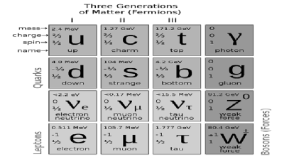
Figure 2.1: Six of the particles in the Standard Model are quarks. Each of the first three columns forms a generation of matter.

In modern particle physics, local gauge symmetries—a kind of symmetry group—determine interactions between particles. Color SU(3) (commonly abbreviated to SU_c(3)) is the gauge symmetry that generated by three color charges which a quark carry and is the defining symmetry for QCD. The requirement that SU_c(3) should be local, i.e its transformations be allowed to vary with space and time—determines the properties of the strong interaction, in particular the existence of eight gluons to act as its force carriers [17].

Properties

The Table 2.1 summarizes the key properties of the six quarks. Flavor quantum numbers ( isospin $(I_{z})$, charmness $(C)$, strangeness $(S$, not to be confused with spin$)$, topness $(T)$, and bottomness $(B)$) are assigned to certain quark flavors, and denote qualities of quark-based systems and hadrons. The baryon number ($\acute{B}$) is $+1/3$ for all quarks, as baryons are made of three quarks. For antiquarks, the electric charge $(Q)$ and all flavor quantum numbers$(B,I_{z},C,S,T,$ $and$ $B)$ are of opposite sign. Quarks are strongly interacting fermions with half integer spin. Quarks have positive intrinsic parity, and are spin 1/2 particles. There are additive flavor quantum numbers for three generations of quarks. Antiquarks have the opposite flavor sign. The charge $Q$ and these quantum numbers are related through the Gell-Mann-Nishijima relation:

$$Q=I_{z}+\frac{\acute{B}+S+C+B+T}{2}$$ (2.1)

where $\acute{B}=1/3,$ is the baryon number for each quark [18].

Table 2.1: Properties of quarks

$Quark\ \backslash\ \Pr operties$ $Q$ $I$ $I_{z}$ $S$ $C$ $B$ $T$ $\acute{B}$ $d$ $-\frac{1}{3}$ $\frac{1}{2}$ $-\frac{1}{2}$ $0$ $0$ $0$ $0$ $\frac{1}{3}$ $u$ $+\frac{2}{3}$ $\frac{1}{2}$ $+\frac{1}{2}$ $0$ $0$ $0$ $0$ $\frac{1}{3}$ $s$ $-\frac{1}{3}$ $0$ $0$ $-1$ $0$ $0$ $0$ $\frac{1}{3}$ $c$ $+\frac{2}{3}$ $0$ $0$ $0$ $+1$ $0$ $0$ $\frac{1}{3}$ $b$ $-\frac{1}{3}$ $0$ $0$ $0$ $0$ $-1$ $0$ $\frac{1}{3}$ $t$ $+\frac{2}{3}$ $0$ $0$ $0$ $0$ $0$ $+1$ $\frac{1}{3}$

                                                                        

2.2 Quark Model

The quark model is a classification scheme for hadrons in term of their valence quarks.

2.2.1 Hadrons

According to the quark model, the properties of hadrons are primarily determined by their valence quarks. Although quarks also carry color charge, hadrons must have zero color charge because of a phenomena called color confinement. That is, hadrons must be ”colorless” or ”white”. There are two ways to accomplish this: three quarks of different colors, or a quark of one color and an antiquark carrying the corresponding anticolor. Hadrons based on the former are called baryons (half odd integer spin), and those based on the latter are called mesons (integer spin). This is possible because of the remarkable property that a singlet exists in $3\otimes 3\otimes 3=1\oplus 8\oplus 8\oplus 10$ as well as in $3\otimes\bar{3}=1\oplus 8$. All hadrons are labelled by quantum numbers. One set comes from the Poincaré symmetry- $J^{PC}$, where $J$, $P$  and  $C$  stand for the total angular momentum, Parity, and Charge-symmetry respectively. Hadrons with same $J^{P}$ (lowest lying as well as higher mass states) are distinguished from each other by some internal quantum numbers. These are flavor quantum numbers such as the isospin, strangeness, charm, and so on. All quarks carry an additive, conserved quantum number called a baryon number, which is +1/3 for quarks and -1/3 for antiquarks. This means that baryons (groups of three quarks) have B = 1 while mesons have B = 0. Hadrons have excited states known as resonances. Each ground state hadron may have several excited states. Resonances decay extreme quickly (within about $10^{-24}$ seconds) via the strong nuclear force [16].

2.2.2 Baryons

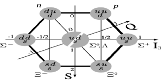
Figure 2.2: Combinations of three $u,d$ or $s$ quarks forming baryons with a spin $1/2$ form the $uds$ baryon octet.

Figure 2.3: Combinations of three $u,d$ or $s$ quarks forming baryons with a spin $3/2$ from the $uds$ baryon decuplet.

2.2.3 Exotic Baryons

Exotic baryons are hypothetical composite particles which are bound states of 3 quarks and additional elementary particles. The additional particles may include quarks, antiquarks or gluons. One such exotic baryon is the pentaquark, which consists of four quarks and an antiquark (B́= 1), but their existence is not generally accepted. Theoretically, heptaquarks (5 quarks, 2 antiquarks), nonaquarks (6 quarks, 3 antiquarks), etc. could also exist. Another exotic baryon which consists only of quarks is the H dibaryon, which consists of two up quarks, two down quarks and two strange quarks. Unlike the pentaquark, this particle might be long lived or even stable. There have been unconfirmed claims of detections of pentaquarks and dibaryons [19].

2.2.4 Mesons

The main difference between mesons and baryons is that mesons are bosons (which obey Bose-Einstein statistics) while baryons are fermions (which obey Fermi-Dirac statistics). Since mesons are composed of quarks, they participate in both the weak and strong interactions. Mesons with net electric charge also participate in the electromagnetic interaction. They are classified according to their quark content, total angular momentum, parity, and various other properties such as $C-$parity and $G-$parity. They are also typically less massive than baryons, meaning that they are more easily produced in experiments, and exhibit higher energy phenomena sooner than baryons would. For example, the charm quark was first seen in the J/Psi meson ($J/\Psi$) in 1974, and the bottom quark in the upsilon meson ($\Upsilon$) in $1977$ [20].

Classification Of Mesons

The mesons are classified in $J^{PC}$ multiplets. The allowed quantum numbers for $L$ smaller than $3$ are given in table. Interestingly, for $J$ smaller than $3$, all allowed $J^{PC}$ except $2^{--}$  have been observed [16].

Table 2.2: Classification of mesons

$L$ $S$ $J^{PC}$ $L$ $S$ $J^{PC}$ $L$ $S$ $J^{PC}$ $0$ $0$ $0^{-+}$ $1$ $0$ $1^{+-}$ $2$ $0$ $2^{-+}$ $0$ $1$ $1^{--}$ $1$ $1$ $0^{++}$ $2$ $1$ $1^{--}$ $1$ $1$ $1^{++}$ $2$ $1$ $2^{--}$ $1$ $1$ $2^{++}$ $2$ $1$ $3^{--}$

Particle physicists are most interested in mesons with no orbital angular momentum $(L=0)$, therefore the two groups of mesons most studied are the $S=1;$ $L=0$ and $S=0;$ $L=0$, which corresponds to $J=1$ and $J=0$, although they are not the only ones. It is also possible to obtain $J=1$ particles from $S=0$ and $L=1$. How to distinguish between the $S=1,$ $L=0$ and $S=0,$ $L=1$ mesons is an active area of research in meson spectroscopy.

For lighter up, down, and strange quarks the suitable mathematical group is $SU(3)$. The quarks lie in the fundamental representation, $3$ (called the triplet) of flavor $SU(3)$. The antiquarks lie in the complex conjugate representation $\bar{3}$. The nine states (nonet) made out of a pair can be decomposed into the trivial representation, $1$ (called the singlet), and the adjoint representation, $8$ (called the octet). The notation for this decomposition is $3\otimes\bar{3}=8\oplus 1$. There are generalizations to larger number of flavors. Charm quark is icluded by extending$\ SU(3)$ to $SU(4)$ [16].

Types Of Mesons

The rules for classification are presented below, in Table 2.3 for simplicity [21].

Table 2.3: Types of mesons

$L$	$J^{PC}$	$Type$	$L$	$J^{PC}$	$Type$
$0$	$0^{-+}$	$pseudoscalars$	$1$	$0^{++}$	$scalars$
$0$	$1^{--}$	$vectors$	$1$	$1^{++},1^{+-}$	$axial\text{ }vectors$
			$1$	$2^{++}$	$tensors$

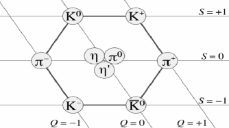
Figure 2.4: Combinations of one $u,$ $d$ or $s$ quarks and one $u$, $d$ or $s$ antiquark in $J^{P}=0^{-}$ configuration form a nonet.

Figure 2.5: Combinations of one $u,$ $d$ or $s$ quarks and one $u$, $d$ or $s$ antiquark in $J^{P}=1^{-}$ configuration form a nonet.

Flavorless mesons are mesons made of quark and antiquark of the same flavor (all their flavor quantum numbers are zero. Flavorful mesons are mesons made of pair of quark and antiquarks of different flavors.

2.3 Mesons And Symmetries

Most of the symmetries in elementary-particle physics are continuous. A typical example is the symmetry generated by rotations around an axis, where the angle of rotation can assume any value between $0$ and $2\pi$. In addition to continuous symmetries, there are also discrete symmetries, for which the possible states assume discrete values classified with the help of a few integers. In elementary-particle physics there are three discrete symmetries of basic importance: parity, charge conjugation and time-reversal.

Spin (quantum number $S$) is a vector quantity that represents the ”intrinsic” angular momentum of a particle. Since quarks are fermi particles of spin $1/2$ $(S=1/2)$ and mesons are made of one quark and one antiquark, they can be found in triplets and singlets spin states. The orbital angular momentum (quantum number L), that comes in increments of $1\hslash$, represent the angular moment due to quarks orbiting around each other. The total angular momentum (quantum number J) of a particle is the combination of intrinsic angular momentum (spin) and orbital angular momentum. It can take any value from $J=|L-S|$ to $J=|L+S|$, in increments of $1$.

2.3.1 C- and P- parity, and Isospin

An important property of any quark state is the behavior of its wave-funtion under certian transformations. One important transformation is the replacement of particle with anti-particle, called C-cojugation. An other one, called P-transformation, is the switching the signs of all coordinates. Many states, but not all, are eigenstates of these two transformations. This means that:

$$\Phi^{\prime} = C\Phi=\lambda_{C}\Phi$$

$$\Phi^{\prime} = P\Phi=\lambda_{P}\Phi$$

The former is possible for the states which are flavor neutral, e.g. electrically neutral. These numbers, $\lambda_{C}$ and $\lambda_{P}$, are called the $C$-parity and $P$- parity of the particular quark state respectively. These transformations have one special property:

$$C^{2}\Phi = \lambda_{C}^{2}\Phi=\Phi$$ (2.2)

$$P^{2}\Phi = \lambda_{P}^{2}\Phi=\Phi$$ (2.3)

It follows that the particular quark state may have $C$

or $P-$parity either $+1$ or $-1$. For example, the $P-$parity of $\pi-$mesons is $-1$:

$$P\pi^{0}=-\pi^{0},P\pi^{+}=-\pi^{+},P\pi^{-}=-\pi^{-}$$

Here $\pi$ stands for the $\pi-$meson wavefuntion. The $C-$parity for $\pi^{0}$ is $+1$, $C\pi^{0}=+\pi^{0};$ but $\pi^{+}$ and $\pi^{-}$ do not have definite $C-$parity, i.e. $C\pi^{+}=+\pi^{-},$ $C\pi^{-}=+\pi^{+}.$

For the system of a quark and an antiquark $(q\bar{q})_{L}$ [note that $q$ and $\bar{q}$ have opposite intrinsic parities], one has

$$P=(-1)\left(-1\right)^{L},\text{ }C=\left(-1\right)^{L+S}\text{\ \ \ \ }$$ (2.4)

For states composite of integer spin bosons these formulae are different. For example, for $\pi^{+}\pi^{-}$ system where pions have zero spin and same intrinsic parities.

$$P=C=\left(-1\right)^{L}$$ (2.5)

An important property of  $C$ and $P-$parities is that they are conserved in the strong and electromagnetic interactions [22]. A generalization to $C-$parity is $G-$parity $G=\left(-1\right)^{L+S+I}$ for mesons. The isospin of $u$ and $d$ quarks is equal to $1/2$, with $u$ quark having positive isospin projection $I$ ${}_{z}=1/2$, and $d$ quark with $I$ ${}_{z}=-1/2$. All other quarks have zero isospin and same holds for a state which is made up of these quarks. For example the isospin of any charmonium state is zero. In particular, isospin becomes crucial when we discuss the possible assignment for the $X\left(3872\right),$ which is assumed to tetraquark state. Isospin $I$ is another property of quark-antiquark system, which is conserved in strong interactions and follow the same algebraic rules as the regular spin $S$. Hadron with nearly same mass can be put into isospin multiplets:

Table 2.4: Isospin Multiplets

$I=\frac{1}{2}$ $\left(\begin{tabular}[]{l}$p$\\ $n$\end{tabular}\right),$ $\ \left(\begin{tabular}[]{l}$K^{+}$\\ $K^{0}$\end{tabular}\right)$ $I_{z}=+\frac{1}{2}$ $\ \ =-\frac{1}{2}$ $I=1$ $\left(\begin{tabular}[]{l}$\Sigma^{+}$\\ $\Sigma^{0}$\\ $\Sigma^{-}$\end{tabular}\right),$  $\left(\begin{tabular}[]{l}$\pi^{+}$\\ $\pi^{0}$\\ $\pi^{-}$\end{tabular}\right)$ $I_{z}=1$ $\ \ \ =0$ $\ \ \ =-1$

Isospin is conserved in strong interaction and as such in that limit, member of each multiplet will have the same mass. The small difference then arises due to electromagnetic interaction, which still conserves $I_{z}$, since $Q=I_{z}+isoscalar$ and charge conservation then implies $I_{z}$ conservtion and/or $m_{u}$ $\neq m_{d}$. This is illustrated by the following decay.

$$\Sigma^{0}|I=1,I_{3}=0\rangle\rightarrow\Lambda\gamma|I=0,I_{3}=0\rangle$$

Isospin and its third component are not conserved in the weak interaction, as demonstrated in the decay:

$$\Lambda|0,0\rangle\rightarrow\pi^{-}p|1,-1\rangle|\frac{1}{2},-\frac{1}{2}\rangle=\sqrt{\frac{1}{3}}|\frac{3}{2},\frac{1}{2}\rangle-\sqrt{\frac{2}{3}}|\frac{1}{2},-\frac{1}{2}\rangle$$

2.3.2 Isospin Symmetry

Isospin symmetry, which is an exact symmetry as for as strong interaction is concerned, is broken by electromagnetic interaction and/or $m_{u}$ $\neq m_{d}$. Thus QCD Lagrangian has isospin symmetry. If $m_{u}$ $=m_{d}=0$ the QCD Lagrangian has chiral symmetry. Since $m_{u}\approx m_{d}<<\Lambda_{QCD}$, the symmetry of the QCD lagrangian is broken when $m_{u}$ $=m_{d}\neq 0$.

2.3.3 Isospin, Charge and Flavor Quantum Numbers

The pion particle had three “charged states”, it was said to be of isospin $I=1$. Its “charged states” $\pi^{+}$, $\pi^{0}$, and $\pi^{-}$, corresponded to the isospin projections $I_{z}=+1,$ $I_{z}=0,$ and $I_{z}=-1$ respectively. Another example is the “rho particle”. Isospin projections were related to the up and down quark content of particles by the relation

$$I_{z}=\frac{1}{2}[(n_{u}-n_{\bar{u}})-(n_{d}-n_{\bar{d}})]$$ (2.6)

where the n’s are the number of up and down quarks and antiquarks.

It was noted that charge $(Q)$ was related to the isospin projection ($I$ _z), the baryon number $(B)$ and flavor quantum numbers $(S,C,\acute{B},T)$ by the Gell-Mann–Nishijima formula. Strangeness flavor quantum number $S$ (not to be confused with spin). Flavor quantum numbers of composites are related to the number of strange, charm, bottom, and top quarks and antiquark according to the relations:

$$S = -(n_{s}-n_{\bar{s}})$$

$$C = +(n_{c}-n_{\bar{c}})$$

$$\acute{B} = -(n_{b}-n_{\bar{b}})$$

$$T = +(n_{t}-n_{\bar{t}})$$

This implies that the Gell-Mann–Nishijima formula is equivalent to the expression of charge in terms of quark content [23].

$$Q=\frac{2}{3}[(n_{u}-n_{\bar{u}})+(n_{c}-n_{\bar{c}})+(n_{t}-n_{\bar{t}})]-\frac{1}{3}[(n_{d}-n_{\bar{d}})+(n_{s}-n_{\bar{s}})+(n_{b}-n_{\bar{b}})]$$ (2.7)

2.4 Exotic Meson

From the quantum numbers in Table 2.1-2.3, there are several combinations which are missing:

$$0^{+-},0^{--},1^{-+}\text{ \ \ and }2^{+-}$$

These are not possible for simple $q\bar{q}$ systems and are known as ”exotic” states. Beyond the simple quark model picture of mesons, there are different frameworks suggested to accomodate these states with exotic quantum numbers. Non-quark model mesons include:

1. glueballs or gluonium, which have no valence quarks at all;

2. tetraquarks, which have two valence quark-antiquark pairs; and

3. hybrid mesons, which contain a valence quark-antiquark pair and one or more gluons.

All of these can be classfied as mesons, because they carry zero baryon number. Of these, glueballs must be flavor singlets; that is, have zero isospin, strangeness, charm, bottomness, and topness. Like all particle states, they are specified by the quantum numbers $J^{PC}$ and by the mass. One also specifies the isospin $I$ of the meson. It is an old idea that the light scalar mesons a($980$) and f($980$) may be 4-quark bound states. The idea was more or less accepted in the mid-seventies but then it losts momentum, due to contradictory results. If the lightest scalar mesons are diquark-antidiquark composites as shown below, it is natural to consider analogous states with one or more heavy constituents, to be discussed in the following section.

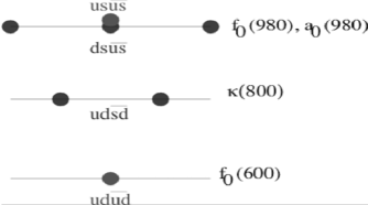
Figure 2.6: Identities and classification of possible tetraquark mesons. First horizontal line denotes I = 0 states, second, I = 1/2 and third one, I = 1. The vertical axis is the mass.

2.5 Diquarks: An Introduction

The notion of the diquark usually means the system of two rather tightly bounded quarks with a small size of$\ 0.1-0.3$ Fermi [25]. This section is devoted to diquarks and their role in understanding exotics in QCD. Diquarks are not new, they are almost as old as QCD. Gell-Mann mentions it prominently in his first paper on quarks in $1964$ [26].

Baryons can be constructed from quarks by using the combinations $(qqq),$ $(qqqq\bar{q})$ etc, while mesons are made out of $\ (q\bar{q}),$ $(qq\bar{q}\bar{q}),$ etc. The lowest baryon configuration $(qqq)$ gives just the representations $1,$ $8,$ and $10$ that have been observed, while the lowest meson configuration $(q\bar{q})$ similarly gives just $1$ and $8$.

The constituents of the tetraquarks, diquarks and antidiquarks, have well-defined properties, characterized by their color and electromagnetic charges, spin and flavor quantum numbers. The tetraquark hadrons are singlets in color (pictured white), and hence they participate as physical states in scattering and decay processes. This is not too dissimilar a situation from the well-known mesons, which are color singlet (white) bound states of the confined colored quarks and antiquarks.

We follow the suggestion by Jaffe and Wilczek $(1977)$ of having diquark as building blocks [15]. Diquark correlations in hadrons suggest qualitative explanations for many of the puzzles of exotic hadron spectroscopy. Operators that will create a diquark of any (integer) spin and parity can be constructed from two quark fields and insertions of the covariant derivative. We are interested in potentially low energy configurations, so we omit the derivatives. There are eight distinct diquark multiplets (in color$\times$flavor$\times$spin), which are enumerated by R. L.Jaffe. Since each quark is a color triplet, the pair can form a color $\bar{3}_{c}$, which is antisymmetric, or $6_{c}$, which is symmetric. The same is true in SU(3)-flavor. The constructions look more familiar if we represent one of the quarks by the charge conjugate field: $qq\rightarrow\bar{q}_{c}q$, where $\bar{q}_{c}=-iq^{T}\sigma^{2}\gamma_{5}$. Then the classification of diquark bilinears is analogous to the classification of $q\bar{q}$ bilinears. There are only two favored configurations. The most attractive channel in QCD seems to be the color antitriplet, flavor antisymmetric (which is the $\bar{3}_{f}$ for three light flavors), spin singlet with even parity: $[qq]^{\bar{3}_{c},\bar{3}_{f},0^{+}}.$ This channel is favored by one gluon exchange and by instanton interactions [27]. It will play the central role in the exotic drama.

$$|\{qq\}\bar{3}_{c}(A)\bar{3}_{f}(A)0^{+}(A)\rangle\text{ \ \ good diquarks}$$ (2.8)

$$|\{qq\}\bar{3}_{c}(A)6_{f}(S)1^{+}(S)\rangle\text{ \ \ bad diquarks}$$ (2.9)

Both of these configurations are important in spectroscopy. Now we can construct the operators for ”good” scalar diquarks and ”bad” vector diquarks [9]. Heavy-light diquarks can be the building blocks of a rich spectrum of states which can accommodate some of the newly observed charmonium-like resonances not fitting a pure $c\bar{c}$ assignment.

$$\mathbf{Q}_{ia} = \epsilon_{ijk}\epsilon_{abc}(i\sigma_{2})q^{jb}q^{kc}=\epsilon_{ijk}\epsilon_{abc}(\bar{q}_{c}^{jb}\gamma_{5}q^{kc})$$ (2.10)

$$\mathbf{\acute{Q}}_{a}^{ij} = \epsilon_{abc}(\bar{q}_{c}^{jb}\vec{\gamma}q^{ic}+\bar{q}_{c}^{ib}\vec{\gamma}q^{jc})$$ (2.11)

Both represent positive parity, $0^{+}$ and $1^{+}$, states. We work out the diquark masses in quark model, in which all residual quark interactions are incorporated. Diquarks are, of course, colored states, and therefore not physical. The good (scalar) and bad (vector) diquarks configurations are our main interest.

2.6 Tetraquark

A tetraquark is a hypothetical meson composed of four valence quarks. In principle, a tetraquark state may be allowed in Quantum chromodynamics, the modern theory of strong interactions. Examining the color algebra of the system reveals there are two independent tetraquark singlet states: $3\otimes\bar{3}\otimes 3\otimes\bar{3}$ $=27\oplus 10\oplus 10\oplus 8\oplus 8\oplus 8\oplus 8\oplus 1\oplus 1$. But they can be obtained in four different ways, depending on the intermediate color states: the singlet scheme (or molecule), the octet scheme, the triplet scheme and the sextet scheme.

Figure 2.7: Singlets can be obtained via four different schemes (only two are independent): octet, singlet (or molecule), sextet and triplet.

A diquark is either in symmetric color state $6_{c}$ or color antisymmetric state $\bar{3}_{c}$. The antidiquark is either in antisymmetric color state $\bar{6}_{c}$ or color symmetric state $3_{c}$. Now

$$6_{c}\otimes\overline{6}_{c} = 35_{c}\oplus 1_{c}$$

$$\overline{3}_{c}\otimes 3_{c} = 8_{c}\oplus 1_{c}$$

$$\overline{3}_{c}\otimes\overline{6}_{c} = \overline{10}_{c}\oplus 8_{c}$$

$$6_{c}\otimes 3_{c} = 10_{c}\oplus 8_{c}$$

Hence only $6_{c}\otimes\overline{6}_{c}$ and $\overline{3}_{c}\otimes 3_{c}$ give color singlet state.

Now diquark are either in symmetric or antisymmetric in flavor:

$$\left[qq\right] = \frac{1}{\sqrt{2}}(q_{i}q_{j}-q_{j}q_{i})\text{ \ }i,\text{ }j=u\text{, }d,\text{ }s,\text{ }c$$

$$\left\{qq\right\} = \frac{1}{\sqrt{2}}(q_{i}q_{j}+q_{j}q_{i})$$

For antisymmetric color state $\overline{3}_{c}$ or $3_{c}$, Pauli principle requires, overall wave function of diquark or antidiquark to be symmetric in flavor, in space and spin: (s, denote the spin of diquark or antidiquark)

$$\left[qq\right]_{L=0,\text{ }s=0}\text{ \ \ \ };\text{ }P = 1\text{ \ \ \ \ }\left[qq\right]_{L=1,\text{ }s=1}\text{ \ \ \ };\text{ }P=-1$$

$$\left\{qq\right\}_{L=0,\text{ }s=1}\text{ \ \ \ };\text{ }P = 1\text{ \ \ \ \ }\left\{qq\right\}_{L=1,\text{ }s=0}\text{ \ \ \ };\text{ }P=-1$$

$$\left[\bar{q}\bar{q}\right]_{L=0,\text{ }s=0}\text{ \ \ \ };\text{ }P = 1\text{ \ \ \ \ }\left[\bar{q}\bar{q}\right]_{L=1,\text{ }s=1}\text{ \ \ \ };\text{ }P=-1$$

$$\left\{\bar{q}\bar{q}\right\}_{L=0,\text{ }s=1}\text{ \ \ \ };\text{ }P = 1\text{ \ \ \ \ }\left\{\bar{q}\bar{q}\right\}_{L=1,\text{ }s=0}\text{ \ \ \ };\text{ }P=-1$$

We have a nonet of low lying scalar mesons $0^{+}$, composite of tetraquark viz

$$\left[qq\right]_{L=0,\text{ }s=0}\ \left[\bar{q}\bar{q}\right]_{L=0,\text{ }s=0}$$

As an example, we consider the following two tetraquark quarkonium states, with $L=0$:

$$\left(\left[qq\right]_{L=0,\text{ }s=0}\left\{\bar{q}\bar{q}\right\}_{L=0,\text{ }s=1}\pm\left\{qq\right\}_{L=0,\text{ }s=1}\left[\bar{q}\bar{q}\right]_{L=0,\text{ }s=0}\right)$$

The two states have $J^{PC\text{ }}=1^{++}$ and $\ 1^{+-}.$ For $q=c$ the $J^{PC\text{ }}=1^{++}$ meson is identified with the state $X(3872)$. This state was reported by the Belle in $2003$. It was suggested as a tetraquark candidate. This state was discovered in the $J/\Psi$ $\pi^{+}\pi^{-\text{ }}$ distribution.

In $2004$ the $D(2632)$ state, seen in the SELEX experiment, was suggested as a possible tetraquark candidate with quark contents $[cd][\bar{d}\bar{s}]$. In $2009$ Fermilab announced that they have discovered a particle temporarily called $Y(4140)$, which may also be a tetraquark with quark contents $[cs][\bar{c}\bar{s}]$ [24].

2.7 QCD, Quarkonia and Hadron Spectroscopy

2.7.1 The Important Physical Properties of QCD

Gluons

The gluons, being mediators of strong interaction between quarks, are vector particles and carry color; both of these properties are supported by hadron spectroscopy.

Color Confinement

Confinement which implies that potential energy between color charges increases linearly at large distances so that only color singlet states exist, a property not yet established but find support from lattice simulations and qualitative pictures. The reasons for quark confinement are somewhat complicated; no analytic proof exists that quantum chromodynamics should be confining, but intuitively, confinement is due to the force-carrying gluons having color charge.

Asymptotic Freedom

Asymptotic freedom which implies that the effective coupling constant $\alpha_{s}=\frac{g_{s}^{2}}{4\pi}$ decreases logarithmically at short distances or high momentum transfers, a property which has a rigorous theoretical basis. This is the basis for perturbative QCD which is relevant for processes involving large momentum transfers. we have

$$\alpha_{s}(Q^{2})=\frac{2\pi}{(11-\frac{2}{3}n_{f})\ln\frac{Q^{2}}{\Lambda_{QCD}^{2}}}$$ (2.12)

the running of $\alpha_{s}(Q^{2})$ with $Q^{2}.\Lambda_{QCD}$ is the QCD scale factor which effectively defines the energy scale at which the running coupling constant attains its maximum value. For $\frac{2}{3}n_{f}$ $<11$, it is clear that $\alpha_{s}(Q^{2})$ decreases as $Q^{2}$ increases and approaches zero as $Q^{2}\rightarrow\infty$ or $r\rightarrow 0$. This is known as the asympotic freedom property of QCD [22].

2.7.2 Quarkonia And Hadron Spectroscopy

Quarkonium designates a flavorless meson whose constituents are a quark and its own antiquark i-e $Q\bar{Q},$ $Q=c,b$, is called quarkonium e.g. charmonium $c\bar{c}$, bottomonium $b\bar{b}$ . Examples of quarkonia are the $J/\Psi$ and $\Upsilon(nS)$ . Because of the high mass of the top quark, a toponium does not exist, since the quark decays through the electroweak interaction before a bound state can form.

For many reasons the strong interactions of hadrons containing heavy quarks are easier to understand than those of hadrons containing only light quarks. The first is asymptotic freedom, the fact that the effective coupling constant of QCD becomes weak in processes with large momentum transfer, corresponding to interactions at short distance scales. At large distances, on the other hand, the coupling becomes strong, leading to nonperturbative phenomena such as the confinement of quarks and gluons on a length scale $R_{had}\sim 1/\Lambda_{QCD}\sim 1fm$, which determines the size of hadrons. Roughly speaking, $\Lambda_{QCD}\sim 0.2GeV\$is the energy scale that separates the regions of large and small coupling constant. When the mass of a quark $Q$ is much larger than this scale, $m_{Q}\gg\Lambda_{QCD}$, it is called a heavy quark.

The light degrees of freedom are blind to the flavor (mass). This is known as flavor symmetry. The heavy quark spin also decouples from the strong interaction. The decoupling of the spin in the heavy quark limit leads to the spin symmetry. These two symmetries have important consequences, especially for the decays of beauty hadrons to lighter hadrons. These symmetries are only true in the heavy quark limit and are violated at order $\frac{\Lambda_{QCD}}{m_{Q}}$.

Since quarks are fermions with spin $1/2$, the wave function is antisymmetric with the exchange of particles $Q$ and $\bar{Q}$. Under particle exchange, we get with space coordinates exchange, a factor $(-1)^{L}$, with spin coordinates exchange, a factor $(-1)^{S+1}$ and with charge exchange, a factor $C$ ($C$ is called $C$-parity). Hence Pauli principle gives

$$(-1)^{L+S+1}C=-1$$ (2.13)

In the spectroscopic notation, state is completely specified as

$$n\text{ }^{2S+1}L_{J}$$ (2.14)

where $n$ is the principal quantum number and $J$ is the total angular momentum. Thus for $L=0$, we have the following states

$$n\text{ }^{1}S_{0}\text{ \ \ }C = +1,\text{ \ \ }n=1,2,....$$

$$n\text{ }^{1}S_{0}\text{ \ \ }C = -1,\text{ \ \ }n=1,2,....$$

The ground state is therefore a hyperfine doublet $1^{1}S_{0}(0^{-+})$ and $1^{3}S_{1}(1^{--})$. For $L=1$, we have the following states

$$n\text{ }^{1}P_{J}\text{ \ \ }J = +1\text{ \ \ \ }C=-1\text{ \ \ }$$

$$n\text{ }^{3}P_{J}\text{ \ \ }J = 0,1,2\text{ \ \ \ }C=1\text{ \ \ }$$

Similarly we can write states for $L=2$.

It is noted that the state ${}^{3}D_{1}$ has the same quantum number as ${}^{3}S_{1}$, therefore they can mix. Most of these states have been discovered experimentally [22]. Some of the states are predicted, but have not been identified; others are unconfirmed.

The computation of the properties of mesons in Quantum chromodynamics (QCD) is a fully non-perturbative one. As a result, the only general method available is a direct computation using Lattice QCD (LQCD) techniques. However, other techniques are effective for heavy quarkonia as well. The speed of the charm and the bottom quarks in their respective quarkonia is sufficiently smaller, so that relativistic effects in these states are much less. This technique is called non-relativistic QCD (NRQCD).

All known hadrons are color singlets. The exchange of gluons can provide binding between quarks in a hadron. The two body one gluon exchange color electric potential is given by:

$$V_{ij} = k_{s}\frac{\alpha_{s}}{r}\text{ },k_{s}=\{-\frac{4}{3}\text{ }for\text{ }q\bar{q},\text{ }$$ (2.15)

$$V_{ij} = k_{s}\frac{\alpha_{s}}{r}\text{ },k_{s}=\{-\frac{2}{3}\text{ }for\text{ }qq$$ (2.16)

Here $i$, $j$ are flavor indices. Since the running coupling constant becomes smaller as we decrease the distance, the effective potential $V_{ij}$ in the lowest order as given by one-gluon exchange potential is a very good approximation for short distances. We conclude that for short distances, one can use the one gluon exchange potential, taking into account the running coupling constant $\alpha_{s}.$ The second regime, i.e. for large $r,$ QCD perturbation theory breaks down and we have the confinement of the quarks. One may look for the origin of this yet unsatisfactorily explained phenomena. There are many pictures which support the existence of a linear confining term. One of them is the string picture of hadrons.

An early, but still effective, technique uses models of the effective potential to calculate masses of quarkonia states. In this technique, one uses the fact that the motion of the quarks that comprise the quarkonium state is nonrelativistic to assume that they move in a static potential, much like nonrelativistic models of the hydrogen atom. One of the most popular potential models is the so-called Cornell potential

$$V(r)=\frac{a}{r}+br$$ (2.17)

where $r$ is the effective radius of the quarkonium state $a$ and $b$ are parameters. The first part, $a/r$ corresponds to the potential induced by one-gluon exchange between the quark and its anti-quark, and is known as the Coulombic part of the potential. The second part, $br$ the linear term is the phenomenological implementation of the confining force between quarks, and parameterizes the poorly-understood non-perturbative effects of QCD. Relativistic and other effects can be incorporated into this approach by adding extra terms to the potential.

Chapter 3 TETRAQUARKS: THE $X\left(3872\right)$

3.1 Facts About The $X\left(3872\right)$

The $X$ was found in an exclusive decay in August $2003$ [1].

$$B^{+}\rightarrow K^{+}X\left(3872\right)\rightarrow K^{+}J/\psi\pi^{+}\pi^{-}$$ (3.1)

Belle measured its mass:

$$m(X\left(3872\right))=3872.0\pm 0.6(stat.)\pm 0.5\text{ }MeV/c^{2}(syst.)$$ (3.2)

Belle also set a limit on its decay width:

$$\Gamma(X\left(3872\right))<2.3\text{ }MeV\text{ }$$ (3.3)

The most natural interpretation was a new coventional$\ c\bar{c}$ state. These exotic states refuse to obey conventional cc̄ charmonium interpretation [2, 3]. So many theories came: molecular models [4, 5], more general 4-quark interpretations including a diquark-antiquark model [6]-[10], hybrid models [11] etc, to explain the nature of the $X\left(3872\right).$ In this chapter we mainly focus on the diquark-antidiquark model.

3.1.1 Charmonium Hypothesis

The fact that the $X\left(3872\right)$ decays to $J/\psi\pi^{+}\pi^{-}$ suggests that it contains $c$ and $\bar{c}$ quarks, and the most natural choice to explain the $X\left(3872\right)$ is an unseen charmonium state. Charmonium system has been thoroughly studied in [30]. After the discovery of the $X\left(3872\right)$ more and more similar narrow resonances have been discovered and confirmed at electron-positron and proton-antiproton colliders. Twenty new unexpected charmonium-like particles have been found which have clear clashes with standard charmonium interpretations. Let us discuss the conventional charmonium states and the main objection for assigning them to the $X(3872).$

The lightest charmonium state is called $\eta_{c}.$ This is the S-state in which the spins of the quarks are antiparallel, so that the total spin is zero and the total angular momentum $J=0.$ The radial quantum number of the $\eta_{c}$ is $n=1$, so that the spectroscopic notation ($n$ ${}^{2S+1}L_{J^{PC}}$) for this state is $1^{1}S_{0}$ and the $J^{PC}$ is $0^{-+}.$ The next, a bit heavier, state is the $J/\psi.$ The next $c\bar{c}$ state $\chi_{c0}$ is a $P-$wave, more exactly $1^{3}P_{0}$, with $J^{PC}=0^{++}.$ This is a part of a triplet, three particles with the same $L$ and $S,$ but different $J.$ The other two particles in the triplet are $\chi_{c1}(1^{3}P_{1^{++}})$ and $\chi_{c2}(1^{3}P_{2^{++}}).$ We discuss the upper part of the spectrum. Only a few of the charmonia states with masses above the $D\bar{D}$ threshold are cosidered. There are a few interesting states e.g. ${}^{1}D_{2}$ and ${}^{3}D_{2}$. The decay of these states into $D\bar{D}$ is forbidden because of their spin-parity $J^{PC}=2^{-\pm}.$ Both $D$ and $\bar{D}$ have zero spin and the spin-parity of the $D\bar{D}$ system is determined by the same way as for two pions. The total even $J$ of $D\bar{D}$ system constrains the $C-$ and $P-$parities to be positive. Therefore these states cannot decay into $D\bar{D}$ and expected to have small widths.

As mentioned earlier that initially the $X\left(3872\right)$ was expected to be one of the so far unknown higher mass charmonium states. However, interpreting the $X\left(3872\right)$ as a conventional state is problematic. We go through all the $c\bar{c}$ states which are not yet identified and evaluate by their suitability for the $X\left(3872\right).$ The states $2S,$ $3P,$ $3D$ and higher are expected to be much heavy to associated with the $X\left(3872\right).$ We do not consider $1S,$ $1P$ and$\ 2S,$ because they are unambiguously identified already. Ten states remain, two of them are known: 1${}^{3}D_{1^{--}}$ is $\psi(3770)$ and $3^{3}S_{1^{--}}$ is $\psi(4040)$, so we will not consider them as serious candidates for the $X\left(3872\right).$ Now the eight states remain. The remaining eight states can not be interpreted as $X$  [18], as mention in the following Table. To be precise, $X\left(3872\right)$ is not a conventional charmonium state.

Table 3.1: Conventional charmonium states and the main objection for assigning them to the $X(3872).$

$1$	$2$	$3$	$4$
$n^{2S+1}L_{J^{PC}}$	Mass $MeV/c^{2}$	$\pi^{-}\pi^{+}$ $J^{PC}$	Main objections for the $X\left(3872\right)$ asignment
$1^{1}D_{2^{-+}}$ $1^{3}D_{2^{--}}$ $1^{3}D_{3^{--}}$	$\sim 3838$ $\sim 3838$ $\sim 3838$	$1^{--}$ $0^{++}$ $0^{++}$	expect $\eta_{c}\pi\pi\gg J/\psi\pi\pi$ not seen decay to $\chi_{c1}\gamma$ not seen decay to $\chi_{c2}\gamma$
$2^{1}P_{1^{+-}}$ $2^{3}P_{0^{++}}$ $2^{3}P_{1^{++}}$ $2^{3}P_{2^{++}}$	$\sim 3968$ $\sim 3932$ $\sim 4008$ $\sim 3966$	0++ 1– 1– 1–	wrong cos$\theta_{J/\psi}$ distribution $D\bar{D}$ not suppressed$\rightarrow$broad too large expected width to $J/\psi\gamma$ $D\bar{D}$ not suppressed$\rightarrow$broad
$3^{1}S_{0^{-+}}$	$\sim 4040$	1–	mass expected to be close to ${}^{3}S_{1}$

3.1.2 Weakly Bound $D-D^{\ast}$ State

There are two possibilities to form bound states out of two quarks and two anti-quarks: In this configuration, binding each quark to an anti-quark $\left[q_{\alpha}\bar{q}^{\alpha}\right]$ and allowing interaction between the two color neutral pairs $\left[q_{\alpha}\bar{q}^{\alpha}\right]\left[q_{\beta}\bar{q}^{\beta}\right]$. Other possible configuration will be discussed in the next section. The mainstream thought has been that of identifying most of these resonances as molecules of charm mesons. In particular the $X\left(3872\right)$ happens to have a mass very close to the $D\bar{D}^{\ast}$ threshold. The binding energy left for the $X\left(3872\right)$ is consistent with $E\thicksim 0.25\pm$ $0.40$ MeV, thus making this state very large in size: order of ten times bigger than the typical range of strong interactions. These questions apply to other near-to-threshold hypothetical molecules and have induced to think to alternative explanations for the $X\left(3872\right)$ and its relatives.

3.2 Diquark-Antidiquark Model

In the diquark-antidiquark model the mass spectra are computed as in the non-relativistic constituent quark model. In the constituent quark model hadron masses are described by an effective Hamiltonian that takes as input the constituent quark masses and the spin-spin couplings between quarks. By extending this approach to diquark-antidiquark bound states it is possible to predict tetraquark mass spectra. The mass spectrum of tetraquarks $\mathcal{Q\bar{Q}}$ with $\mathcal{Q}=[qq]$ can be described in terms of the constituent diquark masses, $m_{\mathcal{Q}}$, spin-spin interactions inside the single diquark, spin-spin interaction between quark and antiquark belonging to two diquarks, spin-orbit, and purely orbital term [6]. This model has been tested on standard charmonia and has a rather good behavior to determine the mass spectra.

3.3 Constituent Quarks and Spin-Spin Interactions

In the costituent quark model the Hamiltonian is [50]:

$$H=\sum\limits_{i}m_{i}+\sum\limits_{i<j}2\mathcal{K}_{ij}(\mathbf{S}_{i}\cdot\mathbf{S}_{j})$$ (3.4)

where the sum runs over the hadron constituents. The coefficient $\mathcal{K}_{ij}$ depends on the flavor of the constituents $i$, $j$ and on the particular color state of the pair. Couplings for color singlet combinations are determined from the scalar and vector light mesons. For the $L=0\$mesons, taking $u\bar{s}$ states, Eq.(3.4) gives

$$M=m_{q}+m_{s}+\mathcal{K}_{s\bar{q}}[J(J+1)-\frac{3}{2}]$$ (3.5)

$$M_{K}=m_{q}+m_{s}+\mathcal{K}_{s\bar{q}}[-\frac{3}{2}]$$

Similarly for the vector meson $K^{\ast}$

$$M_{K^{\ast}}=m_{q}+m_{s}+\mathcal{K}_{s\bar{q}}[1(1+1)-\frac{3}{2}]$$

$$M_{K^{\ast}}=m_{q}+m_{s}+\mathcal{K}_{s\bar{q}}[\frac{1}{2}]$$

$$M_{K^{\ast}}-M_{K}=2\mathcal{K}_{s\bar{q}},\ \mathcal{K}_{s\bar{q}}=195\ MeV$$

Adding the similar equations for $\pi-\rho$, $D-D^{\ast}$, $D_{s}-D_{s}^{\ast}$, $J/\psi-\eta_{c}$ complex we obtain the values of the spin-spin couplings, for quark-antiquark pairs in the color singlet state from known $L=0$ mesons.

Table 3.2: Constituent quark masses derived from the $L=0$ mesons and baryons.

Constituent mass (MeV)	$q$	$s$	$c$	$b$
Mesons	$305$	$490$	$1670$	$5008$
Baryons	$362$	$546$	$1721$	$5050$

Table 3.3: Spin-Spin couplings for quark-antiquark pairs in in the color singlet state from the known mesons.

Spin-spin couplings qq̄ sq̄ ss̄ cq̄ cs̄ cc̄ $(K_{ij})_{0}$(MeV) 318 200 129 71 72 59

Now spin-spin coupling for quark-quark in color $\bar{3}$ (antitriplet) state can be calculated from the known $L=0$ baryons. The $qq$ couplings are determined from the masses of the $qqq$ baryons ground $(J=1/2)$ and excited $(J=3/2)$ states. Lets take the uds states:$\Lambda$, $\Sigma$, $\Sigma^{\ast},$ which gives

$$M=2m_{q}+m_{s}+(\mathcal{K}_{qq})_{{}_{\bar{3}}}[S(S+1)-\frac{3}{2}]+(\mathcal{K}_{qs})_{{}_{\bar{3}}}[J(J+1)-S(S+1)-\frac{3}{4}]$$ (3.6)

Writing equations for $P,$ $\Delta^{+}$, involving only$\ (\mathcal{K}_{qq})_{{}_{\bar{3}}}$, and for $\Lambda_{c},\Sigma_{c},\Sigma_{c}^{\ast}$ , involving $(\mathcal{K}_{qq})_{{}_{\bar{3}}}$ and $(\mathcal{K}_{qc})_{{}_{\bar{3}}}$. Also we consider the three $\Xi_{c}\$states which give $(\mathcal{K}_{qc})_{{}_{\bar{3}}}$ and $(\mathcal{K}_{sc})_{{}_{\bar{3}}}$ couplings. These are given in Table 3.4 where one can see that the coupling strength decreases with increasing mass.

Table 3.4: Spin-Spin couplings for quark-quark in color $\bar{3}$ state from the known baryons.

Spin-spin couplings $qq$ $sq$ $cq$ $cs$ $(K_{ij})_{\bar{3}}$(MeV) $98$ $65$ $22$ $24$

It is observed that the diquark correlation decreases when one of the light quarks is strange. According to one gluon exchange (c.f  Eq.(2.15) and Eq.(2.16)), we have

$$(\mathcal{K}_{ij})_{\bar{3}}=\frac{1}{2}(\mathcal{K}_{ij})_{0}$$ (3.7)

This relates coupling of antitriplet to the singlet state.

The couplings corresponding to the spin-spin interactions have been calculated for the color singlet and color antitriplet only. The couplings are not necessarily in the singlet state but octet couplings $\left(\mathcal{K}_{c\bar{c}}\right)_{8}$ are also possible. The quantities $\mathcal{K}_{q\bar{q}}$, $\mathcal{K}_{c\bar{q}}$ and $\mathcal{K}_{c\bar{c}}$ involve both color singlet and color octet couplings between the quarks and antiquraks in a $\mathcal{Q\bar{Q}}$ system (A quark in the diquark $\mathcal{Q}$ could have a color octet spin-spin interaction with an antiquark in the antidiquark $\mathcal{\bar{Q}}$). For the diquark attraction in the $\bar{3}-$color state, we can write $\mathcal{Q}^{i}=[cq]^{i}=\epsilon^{ijk}c_{j}q_{k}$, where $i,\ j,\ k\$are color indices in the fundamental representation of $SU(3).$ The color singlet hadron is written as

$$[cq][\bar{c}\bar{q}]=\epsilon^{ijk}\epsilon_{ij^{\prime}k^{\prime}}(c_{j}q_{k})(\bar{c}^{j^{\prime}}\bar{q}^{k^{\prime}})=(c_{j}\bar{c}^{j})(q_{k}\bar{q}^{k})-(c_{j}\bar{q}^{j})(q_{k}\bar{c}^{k})$$ (3.8)

Rearranging the color indices in the last term by using $SU(N)$ identity for the Lie algebra generators

$$\sum\limits_{a=1}^{N^{2}-1}\lambda_{ij}^{a}\lambda_{kl}^{a}=2(\delta_{il}\delta_{jk}-\frac{1}{N}\delta_{ij}\delta_{kl})$$ (3.9)

where $N$ is the number of colors. A color octet $(N\ =3)$ $q\bar{q}$ state can be written as $\bar{q}^{i}\lambda_{ij}^{a}q^{j},$ and hence

$$(\bar{c}^{i}\lambda_{ij}^{a}c^{j})(\bar{q}^{k}\lambda_{kl}^{a}q^{l})=\sum\limits_{a=1}^{N^{2}-1}\lambda_{ij}^{a}\lambda_{kl}^{a}(c_{j}\bar{c}^{j})(q_{k}\bar{q}^{k})=2\left[(c_{j}q_{k})(\bar{c}^{j^{\prime}}\bar{q}^{k^{\prime}})-\frac{1}{N}(c_{j}\bar{c}^{j})(q_{k}\bar{q}^{k})\right]$$ (3.10)

Using Eq.(3.9) and Eq.(3.10), we extract the octet term as follows:

$$[cq][\bar{c}\bar{q}] = (c_{j}\bar{c}^{j})(q_{k}\bar{q}^{k})-\left[\frac{1}{2}(\bar{c}^{i}\lambda_{ij}^{a}c^{j})(\bar{q}^{k}\lambda_{kl}^{a}q^{l})+\frac{1}{3}(c_{j}\bar{c}^{j})(q_{k}\bar{q}^{k})\right]$$ (3.11)

$$= \frac{2}{3}(c_{j}\bar{c}^{j})(q_{k}\bar{q}^{k})-\frac{1}{2}(\bar{c}^{i}\lambda_{ij}^{a}c^{j})(\bar{q}^{k}\lambda_{kl}^{a}q^{l})$$ (3.12)

This formula gives information about the relative weights of a singlet and an octet color state in a diquark-antidiquark picture. We have three colors running in the sum $c_{i}\bar{c}^{i}$ whereas $a=1,...,8$ in $\bar{c}^{i}\lambda_{ij}^{a}c^{j}$. Therefore the probability of finding a particular $q\bar{q}$ pair in color singlet, for example $c\bar{c}$ in the color singlet state $c_{j}\bar{c}^{j}$, is half the probability of finding the same pair in color octet $\bar{c}\lambda^{a}c$ i-e, $3\times\ 2/3=1/2(8\times\ 1/2).$

We write for $\mathcal{K}_{c\bar{c}}$ [6]:

$$\mathcal{K}_{c\bar{c}}\left([cq][\bar{c}\bar{q}]\right)=\frac{1}{3}\left(\mathcal{K}_{c\bar{c}}\right)_{0}+\frac{2}{3}\left(\mathcal{K}_{c\bar{c}}\right)_{8}$$ (3.13)

where $\left(\mathcal{K}_{c\bar{c}}\right)_{0}$ is reported in Table 3.3. $\left(\mathcal{K}_{c\bar{c}}\right)_{8}$ can be derived from the one gluon exchange model by using the relation [7]:

$$\left(\mathcal{K}_{c\bar{c}}\right)_{\mathbf{X}}\sim\left(C^{2}\left(\mathbf{X}\right)-C^{2}\left(\mathbf{3}\right)-C^{2}\left(\mathbf{\bar{3}}\right)\right)$$ (3.14)

where $\mathbf{X}$ is the color representation of the two quark system, with $C^{2}\left(\mathbf{X}\right)=0$, $4/3$, $4/3$, $3$ for $\mathbf{X=0}$, $\mathbf{3}$, $\mathbf{\bar{3}}$, $\mathbf{8}$ respectively. It is found that

$$(\mathcal{K}_{c\bar{c}})_{0}\sim-\frac{8}{3}\ \ \ \ \ \ (\mathcal{K}_{c\bar{c}})_{8}\sim\frac{1}{3}=-\frac{1}{8}(\mathcal{K}_{c\bar{c}})_{0}$$ (3.15)

Finally, from Eq.(3.13), one has

$$\mathcal{K}_{c\bar{c}}\left([cq][\bar{c}\bar{q}]\right)=\frac{1}{4}\left(\mathcal{K}_{c\bar{c}}\right)_{0}$$

Now we have all the couplings and let us apply it to calculate the mass of light diquark for a simple case of $a_{0}(980)$:

$$a_{0}(980)=[sq]_{S=0}[\bar{s}\bar{q}]_{S=0}$$

Using the Eq.(3.5) and eigen state given in the above equation, we calculate the mean value

$$\langle a_{0}\left|H\right|a_{0}\rangle = 2m_{[sq]}+(\mathcal{K}_{sq})_{\bar{3}}[-\frac{3}{2}-\frac{3}{2}]=2m_{[sq]}-3(\mathcal{K}_{sq})_{\bar{3}}$$

$$m_{[sq]} = 595\ \ MeV$$

Similarly one can calculate the $m_{[ud]}=396\ \ MeV$ from $\sigma(481)$.

3.4 Spectrum Of Hidden Charm Diquark-antidiquark States

In the diquark-antidiquark model effective Hamiltonian takes the form:

$$H=2m_{\mathcal{Q}}+H_{SS}^{(\mathcal{QQ)}}+H_{SS}^{(\mathcal{Q\bar{Q}\mathcal{)}}}+H_{SL}+H_{LL}$$ (3.16)

where $m_{\mathcal{Q}}$ is the mass of diquark, $H_{SS}^{(\mathcal{QQ)}}$ is the spin-spin interaction inside the single diquark, $H_{SS}^{(\mathcal{Q\bar{Q}\mathcal{)}}}$ is the spin-spin interaction between quark and antiquark belonging to two diquarks, $H_{SL}$ is the spin-orbit, and $H_{LL}$ is purely orbital term [6] i.e

$$H_{SS}^{(\mathcal{QQ)}} = 2(\mathcal{K}_{cq})_{\bar{3}}[(\mathbf{S}_{c}\cdot\mathbf{S}_{q})+(\mathbf{S}_{\bar{c}}\cdot\mathbf{S}_{\bar{q}})],$$ (3.17)

$$H_{SS}^{(\mathcal{Q\bar{Q}\mathcal{)}}} = 2(\mathcal{K}_{c\bar{q}})(\mathbf{S}_{c}\cdot\mathbf{S}_{\bar{q}}+\mathbf{S}_{\bar{c}}\cdot\mathbf{S}_{q})+$$ (3.18)

$$2\mathcal{K}_{c\bar{c}}(\mathbf{S}_{c}\cdot\mathbf{S}_{\bar{c}})+2\mathcal{K}_{q\bar{q}}(\mathbf{S}_{q}\cdot\mathbf{S}_{\bar{q}}),$$

$$H_{SL} = 2A_{\mathcal{Q}}(\mathbf{S}_{\mathcal{Q}}\cdot\mathbf{L}+\mathbf{S}_{\mathcal{\bar{Q}}}\cdot\mathbf{L}),$$ (3.19)

$$H_{LL} = B_{\mathcal{Q}}\frac{L(L+1)}{2}.$$ (3.20)

The overall factor of $2$ is just a convention used in the literature. $A_{\mathcal{Q}},\ B_{\mathcal{Q}}\$are coefficients to be calculated by using known data. We will use these values in the next chapter.

To calculate the spin-spin interaction of the $\mathcal{Q\bar{Q}}$ states explicitly, we use the following non-relativistic notation for labelling the state

$$\left|S_{\mathcal{Q}}\text{,~{}}S_{\bar{\mathcal{Q}}};~{}J\right\rangle=\left|\Gamma\text{,~{}}\Gamma^{\prime};~{}J\right\rangle=(c^{a}\Gamma_{ab}u^{b})(\bar{c}^{c}\Gamma_{cd}^{\prime}\bar{u}^{d})$$ (3.21)

where, $S_{\mathcal{Q}}$ and $S_{\bar{\mathcal{Q}}}$ are the spin of diquark and antidiquark, respectively, $J$ is the total angular momentum and the $\Gamma^{\alpha}$ are $2\times 2$ matrices in spinor space. Using Pauli matrices these can be written as:

$$\Gamma^{0}=\frac{\sigma_{2}}{\sqrt{2}};~{}\Gamma^{i}=\frac{1}{\sqrt{2}}\sigma_{2}\sigma_{i}~{}$$ (3.22)

for spin 0 and 1, respectively. The matrices $\Gamma$ are normalised so that:

$$Tr[(\Gamma^{\alpha})^{\dagger}(\Gamma^{\beta})]=\delta^{\alpha\beta}$$

We define the spinor operators as:

$$\mathbf{S}_{u}\left|\Gamma\right\rangle\equiv\left|\Gamma\frac{1}{2}\sigma\right\rangle;\ \ \ \ \mathbf{S}_{c}\left|\Gamma\right\rangle\equiv\left|\frac{1}{2}\sigma^{T}\Gamma\right\rangle$$

since,

$$\sigma^{T}\sigma_{2}=-\sigma_{2}\sigma$$

We calculated formula for total spin operator as expected:

$$(\mathbf{S}_{u}\mathbf{+\ S}_{c})\left|\Gamma^{0}\right\rangle = 0$$ (3.23)

$$[\mathbf{(S}_{u}\mathbf{)}^{i}\mathbf{+(\ S}_{c}\mathbf{)}^{i}]\left|\Gamma^{j}\right\rangle = i\epsilon^{ijk}\left|\Gamma^{k}\right\rangle$$ (3.24)

We also find:

$$\langle 0|\ \mathbf{S}_{u}\left|1\right\rangle = -\langle 0|\ \mathbf{S}_{c}\left|1\right\rangle=\frac{1}{2};$$ (3.25)

$$\langle 1|\ \mathbf{S}_{u}\left|1\right\rangle = \langle 1|\ \mathbf{S}_{c}\left|1\right\rangle=\frac{1}{2}\langle 1|(\mathbf{S}_{u}\mathbf{+S}_{c})\left|1\right\rangle$$ (3.26)

We have used the following Pauli matrices properties:

$$[\sigma^{i},\sigma^{j}] = 2i\epsilon^{ijk}\sigma^{k}$$

$$Tr(\sigma^{i}\sigma^{i}) = Tr(I)=2$$

By using this information we now calculate the matrix elements of products of spin operators. There are two cases.

Same diquark, e.g.$S_{u}\cdot S_{c}.$

This operator is only a combination of Casimir operators and is diagonal in the basis.

$$2(\mathbf{S}_{u}\mathbf{\cdot S}_{c})=(\mathbf{S}_{cu}\mathbf{)}^{2}\mathbf{-(S}_{c}\mathbf{)}^{2}\mathbf{-(S}_{u}\mathbf{)}^{2}$$ (3.27)

Different diquarks, e.g.$S_{u}\cdot\ S_{\bar{u}}.$First we consider$\ J=0$ states, represented by

$$\left|0_{\mathcal{Q}},0_{\bar{\mathcal{Q}}};~{}0_{J}\right\rangle = \frac{1}{2}\left(\sigma_{2}\right)\otimes\left(\sigma_{2}\right),$$

$$\left|1_{\mathcal{Q}},1_{\bar{\mathcal{Q}}};~{}0_{J}\right\rangle = \frac{1}{2\sqrt{3}}\left(\sigma_{2}\sigma^{i}\right)\otimes\left(\sigma_{2}\sigma^{i}\right),$$

Using the basic definitions, we get:

$$2(\mathbf{S}_{u}\cdot\mathbf{\ S}_{\bar{u}})\left|0_{\mathcal{Q}},0_{\bar{\mathcal{Q}}};~{}0_{J}\right\rangle = \frac{1}{4}\left(\sigma_{2}\sigma^{i}\right)\otimes\left(\sigma_{2}\sigma^{i}\right)=\frac{\sqrt{3}}{2}\left|1_{\mathcal{Q}},1_{\bar{\mathcal{Q}}};~{}0_{J}\right\rangle$$ (3.28)

$$2(\mathbf{S}_{u}\cdot\mathbf{\ S}_{\bar{u}})\left|1_{\mathcal{Q}},1_{\bar{\mathcal{Q}}};~{}0_{J}\right\rangle = \frac{1}{4\sqrt{3}}\left(\sigma_{2}\sigma^{i}\sigma^{j}\right)\otimes\left(\sigma_{2}\sigma^{i}\sigma^{j}\right)$$ (3.29)

$$= \frac{\sqrt{3}}{2}\left|0_{\mathcal{Q}},0_{\bar{\mathcal{Q}}};~{}0_{J}\right\rangle-\left|1_{\mathcal{Q}},1_{\bar{\mathcal{Q}}};~{}0_{J}\right\rangle$$

which leads to the following matrices:

$$2(S_{u}\cdot\ S_{\bar{u}})=\left(\begin{array}[]{cc}0&\frac{\sqrt{3}}{2}\\ \frac{\sqrt{3}}{2}&-1\end{array}\right)$$ (3.30)

Now we consider$\ J=1$ states, given in the tensor basis:

$$\left|0_{\mathcal{Q}},1_{\bar{\mathcal{Q}}};~{}1_{J}\right\rangle = \frac{1}{2}\left(\sigma_{2}\right)\otimes\left(\sigma_{2}\sigma^{i}\right),$$

$$\left|1_{\mathcal{Q}},0_{\bar{\mathcal{Q}}};~{}1_{J}\right\rangle = \frac{1}{2}\left(\sigma_{2}\sigma^{i}\right)\otimes\left(\sigma_{2}\right),$$

$$\left|1_{\mathcal{Q}},1_{\bar{\mathcal{Q}}};~{}1_{J}\right\rangle = \frac{1}{2\sqrt{2}}\varepsilon^{ijk}\left(\sigma_{2}\sigma^{j}\right)\otimes\left(\sigma_{2}\sigma^{k}\right).$$ (3.31)

The normalisation of the Hamiltonian in Eq.(3.16), using the basis of states defined above with definite diquark and antidiquark spin and total angular momentum, will give the spectrum of diquark-antiquark states. There are two different possibilities: Lowest lying $[cq][\bar{c}\bar{q}]$ states $\left(L_{\mathcal{Q\bar{Q}}}=0\right)$ and higher mass $[cq][\bar{c}\bar{q}]$ states $\left(L_{Q\bar{Q}}=1\right)$.

3.4.1 Lowest Lying $[cq][\bar{c}\bar{q}]$ States

In the ground state the two diquarks interact only by spin couplings because the angular momentum is zero $(L_{\mathcal{Q\bar{Q}}}=0)$. An effective non-relativistic Hamiltonian can be written including spin-spin interactions within a diquark and between quarks in different diquarks. The states can be classified in terms of the diquark and antidiquark spin, $S_{\mathcal{Q}}$ and $S_{\bar{\mathcal{Q}}}$, total angular momentum $J$, parity, $P$ and charge conjugation, $C$. Considering both good $(S_{\mathcal{Q}}=0)$ and bad $(S_{\mathcal{Q}}=1)$ diquraks and having $L_{\mathcal{Q\bar{Q}}}=0$ we have six possible states which are listed below.

i. Two states with $J^{PC}=0^{++}$:

$$\left|0^{++}\right\rangle = \left|0_{\mathcal{Q}},0_{\bar{\mathcal{Q}}};~{}0_{J}\right\rangle;$$ (3.32)

$$\left|0^{++\prime}\right\rangle = \left|1_{\mathcal{Q}},1_{\bar{\mathcal{Q}}};~{}0_{J}\right\rangle.$$ (3.33)

ii. Three states with $J=1$:

$$\left|1^{++}\right\rangle = \frac{1}{\sqrt{2}}\left(\left|0_{\mathcal{Q}},1_{\bar{\mathcal{Q}}};~{}1_{J}\right\rangle+\left|1_{\mathcal{Q}},0_{\bar{\mathcal{Q}}};~{}1_{J}\right\rangle\right);$$ (3.34)

$$\left|1^{+-}\right\rangle = \frac{1}{\sqrt{2}}\left(\left|0_{\mathcal{Q}},1_{\bar{\mathcal{Q}}};~{}1_{J}\right\rangle-\left|1_{\mathcal{Q}},0_{\bar{\mathcal{Q}}};~{}1_{J}\right\rangle\right);$$ (3.35)

$$\left|1^{+-\prime}\right\rangle = \left|1_{\mathcal{Q}},1_{\bar{\mathcal{Q}}};~{}1_{J}\right\rangle.$$ (3.36)

All these states have positive parity as both the good and bad diquarks have positive parity and $L_{\mathcal{Q\bar{Q}}}=0$. The difference is in the charge conjugation quantum number, the state $\left|1^{++}\right\rangle$ is even under charge conjugation, whereas $\left|1^{+-}\right\rangle$ and $\left|1^{+-\prime}\right\rangle$ are odd.

iii. One state with $J^{PC}=2^{++}$:

$$\left|2^{++}\right\rangle=\left|1_{\mathcal{Q}},1_{\bar{\mathcal{Q}}};~{}2_{J}\right\rangle.$$ (3.37)

Keeping in mind that for $L_{\mathcal{Q\bar{Q}}}=0$ there is no spin-orbit and purely orbital term, the Hamiltonian of Eq.(3.16) takes the form

$$H=2m_{\mathcal{Q}}+H_{SS}^{(\mathcal{QQ)}}+H_{SS}^{(\mathcal{Q\bar{Q}\mathcal{)}}}$$ (3.38)

Thus,

$$H = 2m_{[qc]}+2(\mathcal{K}_{qc})_{\bar{3}}[(\mathbf{S}_{c}\cdot\mathbf{S}_{q})+(\mathbf{S}_{\bar{c}}\cdot\mathbf{S}_{\bar{q}})]+2\mathcal{K}_{q\bar{q}}(\mathbf{S}_{q}\cdot\mathbf{S}_{\bar{q}})$$ (3.39)

$$+2(\mathcal{K}_{c\bar{q}})(\mathbf{S}_{c}\cdot\mathbf{S}_{\bar{q}}+\mathbf{S}_{\bar{c}}\cdot\mathbf{S}_{q})+2\mathcal{K}_{c\bar{c}}(\mathbf{S}_{c}\cdot\mathbf{S}_{\bar{c}}).$$

The diagonalisation of the this Hamiltonian with the states defined above gives the eigenvalues which are needed to estimate the masses of these states. It is calculated that for the $1^{++}$ and $2^{++}$ states the Hamiltonian is diagonal with the eigenvalues

$$M\left(1^{++}\right) = 2m_{[cq]}-(\mathcal{K}_{cq})_{\bar{3}}+\frac{1}{2}\mathcal{K}_{q\bar{q}}-\mathcal{K}_{c\bar{q}}+\frac{1}{2}\mathcal{K}_{c\bar{c}},$$ (3.40)

$$M\left(2^{++}\right) = 2m_{[cq]}+(\mathcal{K}_{cq})_{\bar{3}}+\frac{1}{2}\mathcal{K}_{q\bar{q}}+\mathcal{K}_{c\bar{q}}+\frac{1}{2}\mathcal{K}_{c\bar{c}}.$$ (3.41)

All other quantities are now specified except the mass of the constituent diquark. The $X(3872)$ is a $[cq]_{S=1}[\bar{c}\bar{q}]_{S=0}$ tetraquark. By diagonalizing the Hamiltonian in Eq.(3.39) and, using the spin couplings derived above, the mass of the diquark $[cq]$ was fixed by using the mass of $X(3872)$ as input, yielding $m_{[cq]}=1.933$ $GeV$. The $1^{++}$ state is a good candidate to explain the properties of $X(3872).$ In order to reduce the experimental information needed we estimate the remaining diquark masses by substituting the costituent quark forming the diquark. We have

$$m_{[cs]} = m_{[cq]}-m_{q}+m_{s}$$ (3.42)

$$m_{[bq]} = m_{[cq]}-m_{c}+m_{b}$$ (3.43)

$$m_{[bs]} = m_{[bq]}-m_{q}+m_{s}$$ (3.44)

Table 3.5: Diquark masses

Diquark masses $[ud]$ $[sq]$ $[cq]$ $[cs]$ $[bq]$ $MeV$ $396$ $595$ $1933$ $2118$ $5119$

Now, we have all the input parameters to calculate the mass spectrum numerically. Putting masses of diquarks from Table (2.4) and values of couplings from Tables (2.2), (2.3) in Eq.(3.40), we get the mass for the hidden $c\bar{c}$ tetraquark $1^{++}$ state:

$$M\left(1^{++}\right)=3.872\text{ }GeV$$ (3.45)

Taking the $X\left(3872\right)$ as input we can also predict the existence of a $2^{++}$ state that can be associated to the  $X\left(3940\right)$ observed by Belle [46]:

$$M\left(2^{++}\right)=3.952\text{ }GeV.$$

For the corresponding $0^{++}$ and $1^{+-}$ (Labelled as $Z$ ) tetraquark states, the Hamiltonian is not diagonal and we calculated the following $2\times 2$ matrices, using the non-relativistic notation for labelling the state as in Eq.(3.30):

$$M\left(0^{++}\right)=\left(\begin{array}[]{cc}-3(\mathcal{K}_{cq})_{\bar{3}}&\frac{\sqrt{3}}{2}\left(\mathcal{K}_{q\bar{q}}+\mathcal{K}_{c\bar{c}}-2\mathcal{K}_{c\bar{q}}\right)\\ \frac{\sqrt{3}}{2}\left(\mathcal{K}_{q\bar{q}}+\mathcal{K}_{c\bar{c}}-2\mathcal{K}_{c\bar{q}}\right)&(\mathcal{K}_{cq})_{\bar{3}}-\left(\mathcal{K}_{q\bar{q}}+\mathcal{K}_{c\bar{c}}+2\mathcal{K}_{c\bar{q}}\right)\end{array}\right),$$

$$M\left(1^{+-}\right)=\left(\begin{array}[]{cc}-(\mathcal{K}_{cq})_{\bar{3}}+\mathcal{K}_{c\bar{q}}-\frac{\left(\mathcal{K}_{q\bar{q}}+\mathcal{K}_{c\bar{c}}\right)}{2}&\mathcal{K}_{q\bar{q}}-\mathcal{K}_{c\bar{c}}\\ \mathcal{K}_{q\bar{q}}-\mathcal{K}_{c\bar{c}}&(\mathcal{K}_{cq})_{\bar{3}}-\mathcal{K}_{c\bar{q}}-\frac{\left(\mathcal{K}_{q\bar{q}}+\mathcal{K}_{c\bar{c}}\right)}{2}\end{array}\right).$$

To estimate the masses of these two states, one has to diagonalise the above matrices. After doing this, the mass spectrum of these states is shown in Fig 3-1.

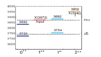
Figure 3.1: Lowest lying hidden charm spectrum.

3.5 Isospin Breaking and Decay Widths of the $J^{PC}=1^{++}$ Tetraquark

3.5.1 Isospin Breaking

In this section we discuss the isospin breaking effects which were neglected in the previous section. The isospin quantum number is related to the finer structure of the $X$ state. The two  flavor eigenstates $X_{u}$ and $X_{d}$ mix through self energy diagrams, which annihilate a $u\bar{u}$ pair and convert it into a $d\bar{d}$ pair through intermediate gluons. In the basis $\{X_{u},X_{d}\}$ the annihilation diagrams contribute equally to all the entries of the mass matrix, while the contribution of the quark masses is diagonal. The resulting $2\times 2$ mixing mass matrix is:

$$\left(\begin{array}[]{cc}2m_{u}+\delta&\delta\\ \delta&2m_{d}+\delta\end{array}\right)$$ (3.46)

where $\delta$ is the contribution from quark annihilation diagrams. At the scale determined by the $c\bar{c}$ pair the annihilation term $\delta$ is expected to be small and thus the mass eigenstates should coincide with  flavor eigenstates to a rather good extent. Isospin-breaking introduces a mass splitting and the mass eigenstates called $X_{[c,l]}$ and $X_{[c,h]}$ (for lighter and heavier of the two) become linear combinations of $X_{[cu]}$ and $X_{[cd]}$. One can put:

$$X_{[c,l]} = \cos\theta\ X_{[cu]}\;+\sin\theta\;X_{[cd]}$$ (3.47)

$$X_{[c,h]} = -\sin\theta\ X_{[cu]}+\cos\theta\ X_{[cd]}$$ (3.48)

The mass differences are estimated to be small, where $\theta$ is a mixing angle. The electromagnetic couplings of the tetraquarks $X_{[c,l]}$ and $X_{[c,h]}$ will depend on the mixing angle $\theta.$

$$\left(\begin{array}[]{c}X_{[c,l]}\\ X_{[c,h]}\end{array}\right)=R\left(\begin{array}[]{c}X_{[cu]}\\ X_{[cd]}\end{array}\right),\text{ }R=\left(\begin{array}[]{cc}\cos\theta&\sin\theta\\ -\sin\theta&\cos\theta\end{array}\right)$$

We get,

$$2m_{u} = M(X_{[c,l]})\cos^{2}\theta+M(X_{[c,h]})\sin^{2}\theta$$

$$2m_{d} = M(X_{[c,l]})\sin^{2}\theta+M(X_{[c,h]})\cos^{2}\theta$$

Take the difference:

$$M(X_{[c,h]})-M(X_{[c,l]})=2(m_{d}-m_{u})/\cos(2\theta)$$ (3.49)

Infact, there are two different states $X(3872)$ and $X(3875)$ which were not excluded from the experimental data [47, 48]. The isospin violation in the tetraquark picture is the possibility of $\omega-\rho^{0}$ mixing, as proposed in [9]. The observation in $2006$ of a state decaying to $D^{0}\bar{D}^{0}\pi$ with mass $3875$ $MeV$ favored the assignment: $X_{u}$ $=X(3875)$, decaying mainly into $J/\psi\pi^{+}\pi^{-}$ and $X_{d}=X(3872)$ decaying into $D^{0}\bar{D}^{0}\pi$. The mass ordering of these two neutral states seems to be reversed, since the $u$ quark is lighter than the $d$ quark and thus one would expect $X_{u}$ to be lighter than $X_{d}$. However the quarks which form the diquarks in the $X_{u}$ have the same electric charge and thus a consistent consideration of the electrostatic energy can perhaps change the order of the masses. Besides these two neutral states, two charged states arise as a natural prediction of the tetraquark picture $X^{+}=[cu][\bar{c}\bar{d}]$ $and$ $X^{-}=[cd][\bar{c}\bar{u}]$. The charged partners are $X^{\pm}$ are not observed [31].

3.5.2 Decay Widths of the $J^{PC}=1^{++}$

Originally the $X(3872)$ was found through its decay into $J/\psi\pi^{+}\pi^{-},$ but other decay modes were also investigate. The decay of a diquark-antidiquark bound state into a pair of mesons can occur through the exchange of a quark and an antiquark belonging respectively to the diquark and the antidiquark. There are indeed three different flavor configurations. Thus we need to introduce three amplitudes. Two of them account for $X\rightarrow D^{0}\bar{D}^{0\ast}$:

Third one the exchange of a light quark and a heavy quark accounts for, the charmonium channels i-e,

$$\text{{A}}\mathbf{([}cq][\bar{c}\bar{q}]\rightarrow[q\bar{q}][c\bar{c}]\mathbf{)}\equiv\text{A}$$ (3.50)

The only available ones are $J/\psi\rightarrow 2\pi$ and $J/\psi\rightarrow 3\pi$, dominated by $\rho^{0}$ and $\omega$ respectively and were confirmed experimentaly.

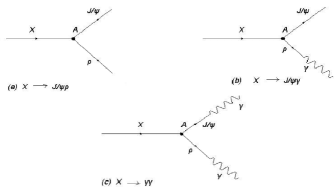
Figure 3.2: Radiative and Hadronic decay of the $X(3872)$ described with the same contact vertex A. The radiative decay proceeds through the hadronic transition.

3.5.3 Hadronic Decays

The decay rate for $X\rightarrow J/\psi+f,$ as shown in Figure 3-2(a) can be written as

$$\frac{d\Gamma(X_{[c,l]}\rightarrow\psi+f)}{ds}=\frac{2x_{l,V}\ |A|^{2}B_{(V\rightarrow f)}}{8\pi M_{X_{[c,l]}}^{2}}.\left[\frac{M_{V}\Gamma_{V}}{\pi}\frac{p(s)}{(s-M_{V}^{2})^{2}+(M_{V}\Gamma_{V})^{2}}\right]$$ (3.51)

with

$$f=\pi^{+}\pi^{-}(\pi^{+}\pi^{-}\pi^{0})\text{ \ for }V=\rho(\omega)$$

$p$ the decay momentum:

$$p(s) = \frac{\sqrt{\lambda(M_{X_{[c,l]}},\ M_{\psi},\ M_{V})}}{2M_{X_{[c,l]}}};$$ (3.52)

$$\lambda = (M_{X_{[c,l]}})^{4}+(M_{\psi})^{4}+(M_{V})^{4}-2(M_{X_{[c,l]}}M_{\psi})^{2}-2(M_{X_{[c,l]}}M_{V})^{2}$$ (3.53)

$$-2(M_{\psi}M_{V})^{2}$$

where the coefficient $x_{l,V}\$is:

$$x_{l,V}\ =\frac{(\cos\theta\ \pm\sin\theta)^{2}\;}{2}$$

and $A$ is taken to be $2.6$ $GeV\$[9]. Similarly we can derive all above equations for higher mass state $X_{[c,h]}.$ Numerical integration of

$$\langle p\rangle_{\rho}=\left(\frac{M_{\rho}\Gamma_{\rho}}{\pi}\right)\int_{(2m_{\pi})^{2}}^{\infty}ds\ \frac{p(s)}{(s-M_{\rho}^{2})^{2}+(M_{\rho}\Gamma_{\rho})^{2}}$$

$$\langle p\rangle_{\omega}=\left(\frac{M_{\rho}\Gamma_{\rho}}{\pi}\right)\int_{(3m_{\pi})^{2}}^{\infty}ds\ \frac{p(s)}{(s-M_{\omega}^{2})^{2}+(M_{\omega}\Gamma_{\omega})^{2}}$$

gives

$$\langle p\rangle_{\rho}=126\ MeV,\ \ \ \langle p\rangle_{\omega}=22\ MeV$$

$$\Gamma(X_{[c,l]}\rightarrow\psi+\pi^{+}\pi^{-})=\frac{2x_{l,\rho}\ |A|^{2}}{8\pi M_{X_{[c,l]}}^{2}}\langle p\rangle_{\rho}$$

$$\Gamma(X_{[c,l]}\rightarrow\psi+\pi^{+}\pi^{-}\pi^{0})=\frac{2x_{l,\omega}\ |A|^{2}}{8\pi M_{X_{[c,l]}}^{2}}\langle p\rangle_{\omega}$$

$$\Gamma(X_{[c,l]} \rightarrow \psi+\pi^{+}\pi^{-})=2x_{l,\rho}\cdot 2.3\ MeV=3.78\text{ }MeV$$ (3.54)

$$\Gamma(X_{[c,l]} \rightarrow \psi+\pi^{+}\pi^{-}\pi^{0})=2x_{l,\omega}\cdot 0.4MeV=0.66\text{ }MeV$$ (3.55)

Using these values of decay rates, we can get the information about the mixing angle $\theta$.

$$\left(\frac{\Gamma(3\pi)}{\Gamma(2\pi)}\right)_{X_{[c,l]}} = \frac{(\cos\theta\ +\sin\theta)^{2}}{(\cos\theta\ -\sin\theta)^{2}}\cdot\frac{\langle p\rangle_{\omega}}{\langle p\rangle_{\rho}}=0.802$$ (3.56)

$$\left(\frac{\Gamma(3\pi)}{\Gamma(2\pi)}\right)_{X_{[c,h]}} = \frac{(\cos\theta\ -\sin\theta)^{2}}{(\cos\theta\ +\sin\theta)^{2}}\cdot\frac{\langle p\rangle_{\omega}}{\langle p\rangle_{\rho}}=0.802$$ (3.57)

where from the Belle experiment we have

$$\left(\frac{\Gamma(3\pi)}{\Gamma(2\pi)}\right)_{Belle}=0.8\pm 0.3_{stat}\pm 0.1_{syst}$$

Putting every thing together we have $\theta\ =\pm 20^{0}$ , for $X_{[c,l]}$ and $X_{[c,h]}$ respectively. For the charged state $X^{\pm},$ that decay via $\rho$-exchange only: we have

$$\Gamma(X^{\pm}\rightarrow J/\psi\pi^{\pm}\pi^{0})=2|A^{2}|\frac{\langle p\rangle_{\rho}}{8\pi M_{X}^{2}}=4.6\text{ MeV}$$

3.5.4 Radiative Decays

The amplitude for the radiative decay $X$ $\rightarrow$ $J/\psi\gamma$ proceeds through the annihilation of a pair of light quarks into a photon, the hadronic part of the amplitude is the same as in the decay $X\rightarrow$ $J/\psi\pi^{+}\pi^{-}$. The radiative decay proceeds through the hadronic transition $X\rightarrow J/\psi\rho.$ Exploiting the Vector Meson Dominance (VMD), which describe interactions between photons and hadronic matter [32], one can write transition matrix from the Fig. 3-2(b) as:

$$\langle J/\psi\gamma|X\rangle=\langle\gamma|\rho\rangle\frac{1}{m_{\rho}^{2}}\langle J/\psi\rho|X\rangle=\frac{f_{\rho}}{m_{\rho}^{2}}A$$ (3.58)

Thus the partial decay width is:

$$\Gamma(X\rightarrow J/\psi\gamma)=2|A^{2}|\left(\frac{f_{\rho}}{m_{\rho}^{2}}\right)^{2}\frac{1}{8\pi M_{X}^{2}}\frac{\sqrt{\lambda(M_{X},\ M_{\psi},\ 0)}}{2M_{X}}$$ (3.59)

Using $f_{\rho}=0.152$ GeV² [10] we get,

$$\frac{\Gamma(X\rightarrow J/\psi\gamma)}{\Gamma(X\rightarrow J/\psi\pi^{+}\pi^{-})}\sim 0.44$$

which is in agreement with experimental value [28].

$$\frac{\Gamma(X\rightarrow J/\psi\gamma)}{\Gamma(X\rightarrow J/\psi\pi^{+}\pi^{-})}<0.40$$

Similarly it is easy to calculate other radiative decays. The experimental values for these radiative decays are [28]:

$$\frac{\Gamma(X\rightarrow\chi_{c1}\gamma)}{\Gamma(X\rightarrow J/\psi\pi^{+}\pi^{-})} \sim 0.89$$

$$\frac{\Gamma(X\rightarrow\chi_{c2}\gamma)}{\Gamma(X\rightarrow J/\psi\pi^{+}\pi^{-})} \sim 1.1$$

We exploit the result obtained for the width of $X$ $\rightarrow$ $J/\psi\gamma$ to give an estimate of the decay width into $J/\psi\gamma\gamma$. We compute the transition matrix element in terms of A using the coupling of the $J/\psi$ to the $\gamma$ for the Figure 3-2(c).

$$\langle\gamma\gamma|X\rangle=\langle\gamma|J/\psi\rangle\frac{1}{m_{J/\psi}^{2}}\langle J/\psi\gamma|X\rangle=\frac{f_{J/\psi}}{m_{J/\psi}^{2}}\langle J/\psi\gamma|X\rangle=\frac{f_{J/\psi}}{m_{J/\psi}^{2}}\frac{f_{\rho}}{m_{\rho}^{2}}A$$ (3.60)

Thus the partial decay width is:

$$\Gamma(X\rightarrow\gamma\gamma)=\frac{4}{3}|A^{2}|\left(\frac{f_{J/\psi}}{m_{J/\psi}^{2}}\right)^{2}\left(\frac{f_{\rho}}{m_{\rho}^{2}}\right)^{2}\frac{1}{8\pi M_{X}^{2}}\frac{\sqrt{\lambda(M_{X},\ 0,\ 0)}}{2M_{X}}$$ (3.61)

Using $f_{J/\psi}=1.254$ GeV² [10] we get,

$$\frac{\Gamma(X\rightarrow\gamma\gamma)}{\Gamma(X\rightarrow J/\psi\pi^{+}\pi^{-})}\sim 3\times 10^{-5}$$

that is greater than the upper limit provided in experimental data [49].

$$\frac{\Gamma(X\rightarrow\gamma\gamma)}{\Gamma(X\rightarrow J/\psi\pi^{+}\pi^{-})}<1.5\times 10^{-5}$$

The inconsistency of the theoretical prediction with respect to data is not dramatic if we take into account the very strong assumptions made to derive the Eq.(3.61).

Chapter 4 GROWING EVIDENCE OF TETRAQUARKS: THE $Y_{b}(10890)$

4.1 Introduction

Using the diquark-antidiquark model, in the previous chapter we learnt to derive the spectrum for lowest lying $[cq][\bar{c}\bar{q}]$ states with $q=u$, $d,$ and discuss the decays of $X(3872)$. This model can be easily applied to lowest lying $[bq][\bar{b}\bar{q}]$ states with $q=u$, $d$, $s$, and $c.$ In this chapter we will discuss the spectrum of the higher mass $[bq][\bar{b}\bar{q}]$ tetraquark states with $q=u$, $d.$ Particularly we are interested in the decays of higher tetraquark particles with $q=u$, $d$. First, there is evidence for $s\bar{s}$ bound state, $Y_{s}(2175)$ having the quantum numbers $J^{PC}=1^{--}$, first observed by BaBar in the initial state radiation $(ISR)$ process $e^{+}e^{-}\rightarrow\gamma_{\mathrm{ISR}}\;f_{0}(980),$ $\phi(1020)$, where $f_{0}(980)$ is the $0^{++}$ scalar state [33]. This was later confirmed by BES [34] and Belle [35]. In December $2007$, the Belle collaboration working at the KEKB $e^{+}e^{-}$ collider in Tsukuba, Japan, reported the first observation of the processes $e^{+}e^{-}\rightarrow Y_{[bq]}\rightarrow\Upsilon(1S,2S)\;\pi^{+}\pi^{-}$ near the peak of the $\Upsilon(5S)$ resonance at the center-of-mass energy of about $10.87$ $GeV$ [12]. Belle measurements near the $\Upsilon(5S)$, however, did not fall in line with theoretical expectations [12]. Their data were enigmatic in the partial decay widths for $\Upsilon(5S)$ $\rightarrow\Upsilon(1S)$ $\pi^{+}\pi^{-}$ and $\Upsilon(2S)$ $\pi^{+}\pi^{-}$ which were typically three orders of magnitude larger than anticipated in QCD [36]. Production and decays of the $\Upsilon(nS)$ states ($n$ being the principal quantum number) are popular theoretical laboratories to test QCD. In particular, the final states $\Upsilon(1S,2S)\;\pi^{+}\pi^{-}$ arising from the production and decays of the lower bottomonia states, such as $\Upsilon(4S)$ $\rightarrow$ $\Upsilon(1S)$ $\pi^{+}\pi^{-}$, have been studied in a number of experiments over the last thirty years and are theoretically well-understood in QCD [36]. In addition, the dipion invariant mass distributions in these events were distinctly different from theoretical expectations as well as from the corresponding measurements at the $\Upsilon(4S)$, undertaken previously by Belle.

In the conventional Quarkonium theory, there is no place for such a nearby additional $b\bar{b}$ resonance having the quantum numbers of $\Upsilon(5S).$ An important issue is whether the puzzling events seen by Belle stem from the decays of the $\Upsilon(5S)$, or from another particle $Y_{b}$ having a mass close enough to the mass of the $\Upsilon(5S)$. We will see that the interpretation of the Belle data is that the anomalous $\Upsilon(1S,2S)\;\pi^{+}\pi^{-}$ events are not due to the production and decays of the $\Upsilon(5S)$, but rather from the production of a completely different hadron species, tetraquark hadrons with the quark structure $Y_{[bq]}=[bq][\bar{b}\bar{q}]$ states with $q=u$, $d$ and their subsequent decays. A. Ali et. al. call this state a ”Brand New Form of Matter”. Identifying the $J^{PC}=1^{--}$ state $Y_{[bq]}(10900)$ seen in the energy scan of the $e^{+}e^{-}\rightarrow b\bar{b}$ cross section by BaBar [31] with the state $Y_{[bq]}(10890)$ seen by Belle [12].

Clearly, two aspects of the Belle data had to be explained:

(a) the anomalously large partial decay rates and

(b) the invariant mass distributions of the dipions.

A dynamical model based on the tetraquark interpretation of $Y_{[bq]}(10890)$ was presented in [38] where it was pointed that it is in agreement with the measured distributions in the decays $Y_{[bq]}\rightarrow\Upsilon(1S)\;\pi^{+}\pi^{-},\Upsilon(2S)\;\pi^{+}\pi^{-}$. They have argued that the decays $Y_{[bq]}\rightarrow\Upsilon(1S,2S)\pi^{+}\pi^{-}$ are radically different than the similar dipion transitions measured in the $\Upsilon(4S)$ and lower mass Quarkonia. Most resently the decays $Y_{[bq]}\rightarrow\Upsilon(1S)K^{+}K^{-}$ was investigated by A. Ali et al. [39] further supporting the Belle data. We will discuss in detail the anomalously large partial decay rates and not the invariant mass distributions of the dipions.

4.2 The Fifth Quark Flavor: Bottom Mesons

Fifth quark was discovered, when in $1977$ the upsilon meson  $\Upsilon(J^{PC}=1^{--})$ was found experimentally as a narrow resonance at Fermi Lab. with mass $\sim 9.5$ GeV. This was later confirmed in $e^{+}e^{-}$ experiments at DESY and CESR which determined its mass to be $9460\pm 10$ MeV and also its width. The updated parameters of this resonance are mass $9460.37\pm 0.21$ MeV and width $52.5\pm 1.8$ keV. Again the narrow width in spite of large phase space available suggests the existence of a fifth quark flavor called beauty, with a new quantum number $B=-1$ for the bottom $(b)$ quark. With this assignment the formula $Q=I_{3}+1/2(Y+B+C)$ would give the charge of $b$ quark the value $-1/3(I_{3}=0)$. The mass of $b$ quark is expected to be around $4.9$ GeV as suggested by the $\Upsilon$ mass which is regarded as a ${}^{3}S_{1}$ bound state of $b\bar{b}$.

One would also expect the particles with $B=\pm 1$, such as $b\bar{q}$ or $q\bar{b}$. The lowest lying bound states $b\bar{q}$ and $q\bar{b}$ have been found experimentally. The $B=-1$ states $(\bar{B}^{0},\,B^{-})\bar{B}_{s}^{0}$ form an SU(3) triplet $(\bar{3})$ and $B=+1$ states $({B}^{+},\,B^{0})B_{s}^{0}$ form another triplet $(3)$. For p-wave multiplets

$(q\bar{b})_{L=1}$	$J^{P}=2^{+},1^{+}$	$\left.\begin{tabular}[]{l}$({B}_{2}^{\ast+,0},\,B_{1}^{+,0})$\\ $({B}_{s_{2}}^{\ast 0},{B}_{s_{1}}^{\ast 0}\,)$\end{tabular}\right]_{j=3/2}$
	$J^{P}=1^{+},0^{+}$	$\left.\begin{tabular}[]{l}$({B}_{1}^{\ast+,0},\,B_{0}^{\ast+,0})$\\ $({B}_{s_{1}}^{\ast 0},{B}_{s_{0}}^{\ast 0})$\end{tabular}\right]_{j=1/2}$

The masses and decay time of B-mesons are given below

$${B}^{\pm} = 5279.16\pm 0.31\text{ }MeV,\text{ \ }\tau=(1.638\pm 0.11)\times 10^{-12}\sec$$

$${B}^{0} = 5279.53\pm 0.33\text{ }MeV,\text{ \ }\tau=(1.530\pm 0.069)\times 10^{-12}\sec$$

4.3 Spectrum Of Higher Mass $[bq][\bar{b}\bar{q}]$ States

For the orbital excitation $L_{Q\bar{Q}}=1$ we consider both good and bad diquarks. The orbital excitation $L_{Q\bar{Q}}=1$ leads to negative parity states,where $1^{--}$ multiplet is of main interest in this chapter. To estimate the masses, we repeat the diagonalization with the basis:

$$\left|1\right\rangle = \left|0_{\mathcal{Q}},0_{\bar{\mathcal{Q}}};~{}1_{J}\right\rangle$$

$$\left|2\right\rangle = \frac{1}{\sqrt{2}}\left(\left|0_{\mathcal{Q}},1_{\bar{\mathcal{Q}}};~{}1_{J}\right\rangle+\left|1_{\mathcal{Q}},0_{\bar{\mathcal{Q}}};~{}1_{J}\right\rangle\right)$$

$$\left|3\right\rangle = \left|1_{\mathcal{Q}},1_{\bar{\mathcal{Q}}};~{}1_{J}\right\rangle$$ (4.1)

Since for the both good and bad diquarks parity is positive as from Eq.(2.8) and Eq.(2.9) ($0^{+}$ and $1^{+}$ respectively), the state $\left|2\right\rangle$ has $P=C=-1$, provided that $L_{Q\bar{Q}}=1.$ Since

$$C_{Q\bar{Q}}(-1)^{L_{Q\bar{Q}}}(-1)^{S_{Q\bar{Q}}}=1$$

therefore for the states $\left|1\right\rangle$ and $\left|3\right\rangle,$ $C_{Q\bar{Q}}=-1$ provided that $S_{Q\bar{Q}}=0,$ $2$ and $L_{Q\bar{Q}}=1.$ First of all we have to change the Hamiltonian given in Eq.(3.16) by replacing the charm quark by bottom quark.

$$H=2m_{\mathcal{Q}}+H_{SS}^{(\mathcal{QQ)}}+H_{SS}^{(\mathcal{Q\bar{Q}\mathcal{)}}}+H_{SL}+H_{LL}$$ (4.2)

where:

$$H_{SS}^{(\mathcal{QQ)}} = 2(\mathcal{K}_{bq})_{\bar{3}}[(\mathbf{S}_{b}\cdot\mathbf{S}_{q})+(\mathbf{S}_{\bar{b}}\cdot\mathbf{S}_{\bar{q}})],$$ (4.3)

$$H_{SS}^{(\mathcal{Q\bar{Q}\mathcal{)}}} = 2(\mathcal{K}_{b\bar{q}})(\mathbf{S}_{b}\cdot\mathbf{S}_{\bar{q}}+\mathbf{S}_{\bar{b}}\cdot\mathbf{S}_{q})+2\mathcal{K}_{b\bar{b}}(\mathbf{S}_{b}\cdot\mathbf{S}_{\bar{b}})+2\mathcal{K}_{q\bar{q}}(\mathbf{S}_{q}\cdot\mathbf{S}_{\bar{q}}),$$ (4.4)

$$H_{SL} = 2A_{\mathcal{Q}}(\mathbf{S}_{\mathcal{Q}}\cdot\mathbf{L}+\mathbf{S}_{\mathcal{\bar{Q}}}\cdot\mathbf{L}),$$ (4.5)

$$H_{LL} = B_{\mathcal{Q}}\frac{L(L+1)}{2}.$$ (4.6)

To perform the digonalization we use the same shorthand notation as described in the previous chapter (c.f. Eq.(3.21) to Eq.(3.30)) for the basis vectors defined in Eq.(4.1). We derive the mass term shift $\Delta m_{SS}$ for higher mass $[bq][\bar{b}\bar{q}]$ states, due to the part of the Hamiltonian containing only spin-spin interaction terms, $H_{SS}.$ Let us first consider

$$(H_{SS})_{33}=\langle 1_{\mathcal{Q}},1_{\bar{\mathcal{Q}}};~{}1_{J}|(H_{SS}^{(\mathcal{QQ)}}+H_{SS}^{(\mathcal{Q\bar{Q}\mathcal{)}}})|1_{\mathcal{Q}},1_{\bar{\mathcal{Q}}};~{}1_{J}\rangle$$

( Here we use $\frac{1}{2}[s_{\mathcal{Q}}(s_{\mathcal{Q}}+1)-\frac{3}{2}]=\vec{S}_{\mathcal{Q}}.\vec{S}_{\mathcal{Q}}$)

$$(H_{SS})_{33} = \langle 1_{\mathcal{Q}},1_{\bar{\mathcal{Q}}};~{}1_{J}|H_{SS}^{(\mathcal{QQ)}}|1_{\mathcal{Q}},1_{\bar{\mathcal{Q}}};~{}1_{J}\rangle+\langle 1_{\mathcal{Q}},1_{\bar{\mathcal{Q}}};~{}1_{J}|H_{SS}^{(\mathcal{Q\bar{Q}\mathcal{)}}}|1_{\mathcal{Q}},1_{\bar{\mathcal{Q}}};~{}1_{J}\rangle$$

$$= 2\left(\mathcal{K}_{bq}\right)_{\bar{3}}(2-3/2)+2\mathcal{K}_{b\bar{q}}[(2-3/2)\frac{1}{2}+(2-3/2)\frac{1}{2}]$$

$$+2\mathcal{K}_{q\bar{q}}(2-3/2)\frac{1}{2}+2\mathcal{K}_{b\bar{b}}(2-3/2)\frac{1}{2}$$

$$= \left(\mathcal{K}_{bq}\right)_{\bar{3}}-\mathcal{K}_{b\bar{q}}-\frac{1}{2}\mathcal{K}_{q\bar{q}}-\frac{1}{2}\mathcal{K}_{b\bar{b}}$$ (4.8)

Similarly we can easily calculate $(H_{SS})_{11}$ and $(H_{SS})_{22}.$ All off diagonal elements are zero. Thus finally we have,

$$\Delta m_{SS}=\left(\begin{array}[]{ccc}-3\left(\mathcal{K}_{bq}\right)_{\bar{3}}&0&0\\ 0&\begin{array}[]{c}-\left(\mathcal{K}_{bq}\right)_{\bar{3}}-\mathcal{K}_{b\bar{q}}\\ +\left(\mathcal{K}_{q\bar{q}}+\mathcal{K}_{b\bar{b}}\right)/2\end{array}&0\\ 0&0&\begin{array}[]{c}\left(\mathcal{K}_{bq}\right)_{\bar{3}}-\mathcal{K}_{b\bar{q}}\\ -\left(\mathcal{K}_{q\bar{q}}+\mathcal{K}_{b\bar{b}}\right)/2\end{array}\end{array}\right)$$ (4.9)

The eigenvalues of the spin-orbit and angular momentum operators given in Eq.(4.5) and Eq.(4.6), were calculated by Polosa et al. [6], we have

$$A_{\mathcal{Q}} = 5\text{ MeV, for }q=u\text{, }d,$$

$$B_{\mathcal{Q}} = 408\text{ MeV, for }q=u\text{, }d,$$

We use these values in order to calculate the numerical values of these states. Hence the eight tetraquark states $[bq][\bar{b}\bar{q}]$ ($q=u,$ $d$) having the quantum numbers $1^{--}$ are:

$$M_{Y_{[bq]}}^{(1)}\left(S_{\mathcal{Q}}=0,~{}S_{\bar{\mathcal{Q}}}=0,~{}S_{\mathcal{Q\bar{Q}}}=0,~{}L_{\mathcal{Q\bar{Q}}}=1\right) = 2m_{\left[bq\right]}+\lambda_{1}+B_{\mathcal{Q}},$$ (4.10)

$$M_{Y_{[bq]}}^{(2)}\left(S_{\mathcal{Q}}=1,~{}S_{\bar{\mathcal{Q}}}=0,~{}S_{\mathcal{Q\bar{Q}}}=1,~{}L_{\mathcal{Q\bar{Q}}}=1\right) = 2m_{\left[bq\right]}+\Delta+\lambda_{2}-2A_{Q}+B_{\mathcal{Q}},$$ (4.11)

$$M_{Y_{[bq]}}^{(3)}\left(S_{Q}=1,~{}S_{\bar{Q}}=1,~{}S_{Q\bar{Q}}=0,~{}L_{Q\bar{Q}}=1\right) = 2m_{\left[bq\right]}+2\Delta+\lambda_{3}+B_{\mathcal{Q}},$$ (4.12)

$$M_{Y_{[bq]}}^{(4)}\left(S_{Q}=1,~{}S_{\bar{Q}}=1,~{}S_{Q\bar{Q}}=2,~{}L_{Q\bar{Q}}=1\right) = 2m_{\left[bq\right]}+2\Delta+\lambda_{3}-6A_{Q}+B_{\mathcal{Q}},$$ (4.13)

where $\lambda$’s are the diagonal elements of the matrix $\Delta M_{SS}$ given in Eq.(4.9). The quantity $\Delta,$ is the mass difference of the good and the bad diquarks i.e.

$$\Delta=m_{\mathcal{Q}}\left(S_{\mathcal{Q}}=1\right)-m_{\mathcal{Q}}\left(S_{\mathcal{Q}}=0\right).$$

and from Eq.(3.43)

$$m_{[bq]}=m_{[cq]}-m_{c}+m_{b}$$

Now one of the remaining unknowns in this calculation is the quantity $\Delta$, the mass difference of the good and the bad diquarks. Following Jaffe and Wilczek [19], the value of $\Delta$ for diquark $[bq]$ is $202$ MeV.

We recall previous chapter where we have used the known mesons and baryons to calculate the couplings of the spin-spin interaction. We can extend the same procedure to the $S=1$, $L=(0$, $1$) meson states $B^{\ast}$, $B_{1}\left(5721\right)$, $B_{2}\left(5747\right)$ to calculate the values:

Table 4.1: Spin-Spin couplings for quark-antiquark pairs in in the color singlet state from the known bottom mesons.

Spin-spin couplings	$q\bar{q}$	$b\bar{q}$	$b\bar{b}$
$\left(\mathcal{K}_{ij}\right)_{0}$(MeV)	$318$	$23$	$36$

Table 4.2: Spin-Spin couplings for quark-quark in color $\bar{3}$ state from the known bottom baryons.

Spin-Spin couplings	$qq$	$bq$
$\left(\mathcal{K}_{ij}\right)_{\bar{3}}$(MeV)	$98$	$6$

Ultimately by putting things together, the masses for the states given in Eqs.(4.10-4.13) are given in Table and can be compared with the ones estimated in refs. [40] using the QCD sum rules.

Table 4.3: Masses of the the $1^{--}$ neutral tetraquark states $M_{{Y}_{[bq]}}^{(n)}$ in GeV. The value $M_{{Y}_{[bq]}^{(1)}}$ (for $q=u,d$) is fixed to be 10.890 GeV, identifying this with the mass of the $Y_{b}$ from BELLE. 

.

$M_{Y_{[bq]}}^{(i)}$ $M_{Y_{[bq]}}^{(1)}$ $M_{Y_{[bq]}}^{(2)}$ $M_{Y_{[bq]}}^{(3)}$ $q=u,d$ $10890$ $11130$ $11257$ $M_{Y_{[bq]}}^{(4)}$ $11227$

Note that there are 8 electrically neutral self-conjugate $1^{--}$ tetraquark states $Y_{[bq]}^{(n)}$ with the quark contents $[bq][\bar{b}\bar{q}]$, with $q=u$, $d$ of which the two corresponding to $[bu][\bar{b}\bar{u}]$ and $[bd][\bar{b}\bar{d}]$, i.e., $Y_{[bu]}^{(n)}$ and $Y_{[bd]}^{(n)}$ are degenerate in mass due to the isospin symmetry. Their mass difference is induced by isospin splitting $m_{d}-m_{u}$, mixing angle $\theta$ and is estimated as $\Delta M(Y_{b})=(5.6\pm 2.8)$ MeV. Due to this small differnce in the following we will not distinguish between the lighter and the heavier of these states and denote them by the common symbol $Y_{b}.$ There are yet more electrically neutral $J^{PC}=1^{--}$ states with the mixed light quark content $[bd][\bar{b}\bar{s}]$ and their charge conjugates $[bs][\bar{b}\bar{d}]$. However, these mixed states don’t couple directly to the photons, $Z^{0}$ or the gluon, and are not of our main interest.

4.4 Decay Widths Of The $Y_{b}(10890)$

4.4.1 Leptonic Decay Widths

For bottomonium systems, the corresponding decay widths are determined by the wave functions at the origin for the $\Upsilon(nS)$, $\Psi_{b\bar{b}}(0)$, and by the derivative of these functions at the origin, $\Psi_{b\bar{b}}^{\prime}(0)$, for the P-waves. To take into account the possibly larger hadronic size of the tetraquarks compared to that of the $b\bar{b}$ mesons, we modify the Quarkonia potential, usually taken as a sum of linear (confining) and Coulombic (short-distance) parts. For example, the Buchmüller-Tye $Q\bar{Q}$ potential [41] has the asymptotic forms

$$V(r) \sim k_{Q\bar{Q}}\;r\text{ },\text{\ \ \ \ \ \ \ \ \ \ \ \ \ \ \ \ \ \ \ \ \ \ }(\text{for }r\rightarrow\infty)$$ (4.14)

$$V(r) \sim 1/r\ln(1/\Lambda_{\mathrm{QCD}}^{2}\;r^{2})\text{ },\text{\ \ \ \ \ \ }(\text{for }r\rightarrow 0)$$ (4.15)

where $k_{Q\bar{Q}}$ is the string tension and $\Lambda_{\mathrm{QCD}}$ is the QCD scale parameter. The bound state tetraquark potential $V_{\mathcal{Q\bar{Q}}}(r)$ will differ from the Quarkonia potential $V_{Q\bar{Q}}(r)$ in the linear part, as the string tension in a diquark $k_{\mathcal{QQ}}$ is expected to be different than the corresponding string tension $k_{Q\bar{Q}}$ in the $Q\bar{Q}$ mesons. The diquarks-antidiquarks in the tetraquarks and the quarks-antiquarks in the mesons are in the same $\bar{3}_{c}3_{c}$ color configuration, the Coulomb (short-distance) parts of the potentials will be similar. Defining,

$$\kappa=k_{\mathcal{Q\bar{Q}}}/k_{Q\bar{Q}}$$ (4.16)

we expect $\kappa$ to have a value in the range $\kappa\in[\frac{1}{2},\frac{\sqrt{3}}{2}]$ [42]. This will modify the tetraquark wave functions $\Psi_{\mathcal{Q\bar{Q}}}(0)$ from the corresponding wave functions of the bound $b\bar{b}$ systems, effecting the decay amplitudes and hence all the decay widths of the tetraquarks. The corresponding value for the tetraquark states $[bq][\bar{b}\bar{q}]$ is then calculated taking into account the ratio of the string tensions $\kappa$. As the linear part of the confining potential determines essentially the heavy Quarkonia wave functions, we find that to a good approximation:

$$\Psi_{\mathcal{Q\bar{Q}}}(0)\simeq\kappa\Psi_{b\bar{b}}(0)$$ (4.17)

which is what we can use in our derivations of the decay widths.

The partial electronic widths $\Gamma_{ee}(Y_{[b,l]})$ and $\Gamma_{ee}(Y_{[b,h]})$ are given by the well known Van Royen-Weisskopf formula for the P-states, which we write as:

$$\Gamma_{ee}=\frac{16\pi Q^{2}\alpha^{2}|\Psi_{\mathcal{Q\bar{Q}}}^{\prime}|^{2}}{M^{2}\omega^{2}},$$ (4.18)

where $Q=-2/3$ is the diquark charge in $Y_{bd}=[bd][\bar{b}\bar{d}]$ and $Q=+1/3$ is the charge of the diquarks in $Y_{bu}=[bu][\bar{b}\bar{u}]$, $\alpha=1/137$ is the electromagnetic coupling constant to lowest order and $\Psi_{\mathcal{Q\bar{Q}}}^{\prime}(\vec{r})=\psi(\phi,\theta)R^{\prime}(r)$ is the first derivative in $r$ of the wave function of the tetraquark, which needs to be taken at the origin i.e.,

$$\Psi_{\mathcal{Q\bar{Q}}}^{\prime}(\vec{r})=\sqrt{\frac{3}{4\pi}}R^{\prime}(0)$$ (4.19)

The wave function $\Psi_{b\bar{b}}^{\prime}(0)$ depends on the underlying potential model. Tetraquarks are bound state of diquarks-antidiquarks with the same internal color structure as the Quarkonia, i.e. both are $(\mathbf{3}$, $\mathbf{\bar{3}})$ bound states. Hence, they also depend, in principle, on the potential models. We will not distinguish between the lighter and the heavier of these states because their mass difference is induced by isospin splitting $m_{d}-m_{u}$ and a mixing angle and is estimated as $\Delta M(Y_{b})=(5.6\pm 2.8)$ MeV. So we denote them by the common symbol $Y_{b}.$

To calculate the radial wave function, we took the value calculated by using the QQ-onia package [27] yielding $\left|R^{\prime}(0)\right|^{2}=2.062GeV$. Since each derivative increases the energy dimension by and thus we need to normalize by kinetic energy $\omega\approx m_{\mathcal{Q}}$ of the diquark. For the lowest lying $1^{--}$ state we get,

$$\Gamma_{ee}\approx 0.12KeV$$ (4.20)

Since all the $1^{--}$ states are P-waves, the $R^{\prime}(0)$ value will not change because the masses of the diquarks remain the same. So the value of $\Gamma_{ee}$ only varies with the mass and therefore does not change significantly. This value is close to the experimental value given in [31].

4.4.2 Hadronic Decays

We discuss the two-body hadronic decays of the $Y_{b}(10890)$, $Y_{b}(q)\rightarrow B_{q}^{(\ast)}(k)\bar{B}_{q}^{(\ast)}(l)$ . The decays $Y_{b}\rightarrow\Upsilon(1S,2S)\;\pi^{+}\pi^{-}$ are also Zweig allowed. These decays $Y_{[bq]}\rightarrow\Upsilon(1S,2S)\;\pi^{+}\pi^{-}$ are too much phase space suppressed and require a dynamical model, which we will also discuss later.

The Vertices of the dominant two-body hadronic decays of the $Y_{b}(10890)$ are [43]:

$$Y_{b}\rightarrow B\bar{B}$$

(4.21)

The corresponding decay widths are respectively:

$$\;\Longrightarrow\;\;\Gamma\;$$

(4.22)

The decaying momentum $|\vec{k}|$ is as given in Eq.(3.52)

$$|\vec{k}|=\frac{\sqrt{M^{2}-(M_{k}+M_{l})^{2}}\sqrt{M^{2}-(M_{k}-M_{l})^{2}}}{2M},$$ (4.23)

where $M$ is the mass of the decaying particle and $M_{k}$, $M_{l}$ are the masses of the decay products. The matrix elements are obtained by multiplying the vertices by the polarization vectors $\varepsilon^{(i)\mu}$. The polarisation vectors $\varepsilon^{(i)\mu}$ satisfy the transversality condition with the polarisation sum

$$\sum\limits_{i}^{3}\varepsilon^{(i)\mu}(p)\varepsilon^{(i)\nu}(p)=-g^{\mu\nu}+\frac{p^{\mu}p^{\nu}}{p^{2}}$$ (4.24)

Thus, for the decay $Y_{[bq]}\rightarrow B_{q}\bar{B}_{q},$ the Lorentz-invariant matrix element is:

$$\mathcal{M}=\varepsilon_{\mu}^{[bq]}F(k^{\mu}-l^{\mu})$$ (4.25)

The decay constants $F$ are non-perturbative quantities, which are beyond the scope in our approximation. We estimate them using the known two-body decays of $\Upsilon(5S)$, which are described by the same vertices as given Eq.(4.21) [16]. We use the decay widths for the decays $\Upsilon(5S)\rightarrow B\bar{B},B\bar{B}^{\ast},B^{\ast}\bar{B}^{\ast}$ from the PDG, yielding the coupling constants, called $F_{\mathrm{PDG}}$ and $|\vec{k}|.$

Table 4.4: 2-body decays $\Upsilon(5S)\rightarrow B^{(\ast)}\bar{B}^{(\ast)}$, which we use as a reference, with the mass and the decay widths taken from PDG. The extracted values of the coupling constants $F$ and the centre of mass momentum $|\vec{k}|$ are also shown.

Process	$\Gamma_{PDG}\left[MeV\right]$	$F_{PDG}$	$|\vec{k}|\left[GeV\right]$
$\Upsilon(5S)\rightarrow B\bar{B}$	$<13.2$	$<2.15$	$1.3$
$\Upsilon(5S)\rightarrow B\bar{B}^{\ast}$	$15.4_{-6.6}^{+6.6}$	$3.7_{-0.9}^{+0.7}$	$1.2$
$\Upsilon(5S)\rightarrow B^{\ast}\bar{B}^{\ast}$	$48_{-11}^{+11}$	$1_{-0.12}^{+0.13}$	$1.0$

The different hadronic sizes of the $b\bar{b}$ Onia states and the tetraquarks $Y_{[bq]}$ are taken into account by the quantity $\kappa$, discussed earlier.

Table 4.5: Reduced partial decay widths for the tetraquarks $Y_{[bq]}^{(i)}$, the extracted value of the coupling constant $F$ and the centre of mass momentum $|\vec{k}|$. The errors in the entries correspond to the errors in the decay widths in Table 4-5.

Decay Mode	$\Gamma/\kappa^{2}[MeV]$	$F$	$|\vec{k}|[GeV]$
$Y_{[bq]}^{(1)}\rightarrow B\bar{B}$	$<15$	$2.15$	$1.3$
$Y_{[bq]}^{(1)}\rightarrow BB^{\ast}$	$18_{-8}^{+8}$	$3.7$	$1.2$
$Y_{[bq]}^{(1)}\rightarrow B^{\ast}\bar{B}^{\ast}$	$56_{-14}^{+14}$	$1$	$1.1$

Thus, the decay widths of $Y_{[bq]}^{(1)}$ are consistent with the corresponding measurements by Belle. The other three higher $1^{--}$ states have much larger decay widths and will be correspondingly more difficult to find.

4.4.3 Dynamical Model For $Y_{b}\rightarrow\Upsilon(1S,2S)\;\pi^{+}\pi^{-}$

(Introduction and results)

Explaining the larger decay rates for the transitions $Y_{b}(q)\rightarrow\Upsilon(p)+\pi^{+}(k_{1})+\pi^{-}(k_{2})$ was not so difficult, as the decays of $Y_{b}$ involve a recombination of the initial four quarks, as exemplified below by the process $Y_{[bu]}$ $=$ $[bu][\bar{b}\bar{u}]\rightarrow(b\bar{b})(u\bar{u}),$ with the subsequent projection $(b\bar{b})\rightarrow\Upsilon(1S)$ and $(u\bar{u})\rightarrow\pi^{+}\pi^{-}.$Such quark recombination processes do not require the emission and absorption of gluons, and are appropriately called Zweig-allowed, after the co-discoverer of the quark-model, George Zweig. The relevant diagrams for the decays $Y_{b}(q)\rightarrow\Upsilon(p)+\pi^{+}(k_{1})+\pi^{-}(k_{2})$.

The decays $Y_{b}\rightarrow\Upsilon(1S)\;\pi^{+}\pi^{-},\Upsilon(2S)\;\pi^{+}\pi^{-}$ are sub-dominant, but Zweig-allowed and involve essentially the quark rearrangements shown below. With the $J^{PC}$ of the $Y_{b}$ and $\Upsilon(nS)$ both $1^{--}$, the $\pi^{+}\pi^{-}$ states in the decays $Y_{b}\rightarrow\Upsilon(1S)\;\pi^{+}\pi^{-},\Upsilon(2S)\;\pi^{+}\pi^{-}$ are allowed to have the $0^{++}$ and $2^{++}$ quantum numbers. There are only three low-lying states in the Particle Data Group (PDG)  which can contribute as intermediate states, namely the two $0^{++}$ states, $f_{0}(600)$ and $f_{0}(980)$, which, following [44, 45] we take as the lowest tetraquark states, and the $2^{++}$ $q\bar{q}$-meson state $f_{2}(1270)$, all of which decay dominantly into $\pi\pi.$ For the decay $Y_{b}\rightarrow\Upsilon(1S)\;\pi^{+}\pi^{-}$, all three states contribute. However, kinematics allows only the $f_{0}(600)$ in the decay $Y_{b}\rightarrow\Upsilon(2S)\;\pi^{+}\pi^{-}$. This model encodes all these features. Finally the fits of the Belle data with this model, yield the measured partial decay widths $\Gamma_{\Upsilon(1S)+2\pi}=0.59\pm 0.04\pm 0.09~{}$MeV and $\Gamma_{\Upsilon(2S)+2\pi}=0.85\pm 0.07\pm 0.16~{}$MeV [38].

4.4.4 Radiative Decays

The amplitude for the radiative decay $Y_{b}\rightarrow$ $\chi_{b}\gamma$ will proceed through the annihilation of a pair of light quarks into a photon.

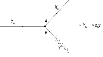
Figure 4.1: Radiative decay of the $Y(10890)$. The radiative decay proceeds through the hadronic transition.

Exploiting the Vector Meson Dominance (VMD), one can write transition matrix from the Fig. 4-1 as:

$$\langle\chi_{b}\gamma|Y_{b}\rangle=\langle\gamma|\rho\rangle\frac{1}{m_{\rho}^{2}}\langle\chi_{b}\rho|Y_{b}\rangle=\frac{f_{\rho}}{m_{\rho}^{2}}A$$

Thus the partial decay width is:

$$\Gamma(Y_{b}\rightarrow\chi_{b}\gamma)=2|A^{2}|\left(\frac{f_{\rho}}{m_{\rho}^{2}}\right)^{2}\frac{1}{8\pi M_{Y_{b}}^{2}}\frac{\sqrt{\lambda(M_{Y_{b}},\ M_{\chi_{b}},\ 0)}}{2M_{Y_{b}}}$$

where $\frac{\sqrt{\lambda(M_{Y_{b}},\ M_{\chi_{b}},\ 0)}}{2M_{Y_{b}}}$ is the decay momentum and the value of $\lambda(M_{Y_{b}},\ M_{\chi_{b}},\ 0)$ is very easy to calculate using Eq.(3.53).

Using $f_{\rho}=0.152$ GeV² given in [10], we get:

$$\frac{\Gamma(Y_{b}\rightarrow\chi_{b}\gamma)}{\Gamma(Y_{b}\rightarrow\Upsilon(1S)\;\pi^{+}\pi^{-})}\sim 0.3$$

Similarly

$$\frac{\Gamma(Y_{b}\rightarrow\eta_{b}\gamma)}{\Gamma(Y_{b}\rightarrow\Upsilon(1S)\;\pi^{+}\pi^{-})}\sim 0.5$$

For $Y_{b}\rightarrow\chi_{b}\gamma$ and $Y_{b}\rightarrow\eta_{b}\gamma,$ the lack of experimental results do not allow us to draw any solid conclusions. However, we have made their theoretical decay rate predictions.

Chapter 5 Conclusion

We have analyzed the spectroscopy of particles with hidden charm and bottom in diquark-antidiquark structures of the kind of ${\mathcal{Q}}{\bar{\mathcal{Q}}}=[\acute{q}q][\overline{\acute{q}}\bar{q}]$, where $q=u$ or $d$ ; $\acute{q}=c$ or $b$, and $\mathcal{Q}$ is a diquark. The idea that the color diquark is handled as a constituent building block is at the core of the approach taken in this dissertation. In this context we used the constituent quark model (CQM) as a benchmark to identify and compare the properties of the newly discovered. Constituent quark models typically assume a QCD motivated potential that includes a Coulomb-like one-gluon-exchange potential at small separation and a linearly confining potential at large separation. In the constituent quark model hadron masses are described by an effective Hamiltonian: $H=\sum\limits_{i}m_{i}+\sum\limits_{i<j}2\mathcal{K}_{ij}(\mathbf{S}_{i}\cdot\mathbf{S}_{j})$ that takes as input the constituent quark masses and the spin-spin couplings between quarks. The coefficient $\mathcal{K}_{ij}$ depends on the flavor of the constituents $i$, $j$ and on the particular color state of the pair. By extending this approach to diquark-antidiquark bound states it is possible to predict tetraquark mass spectra. The mass spectrum of tetraquarks $[\acute{q}q][\overline{\acute{q}}\bar{q}]$ with $q=u$, $d$ and $\acute{q}=c$, $b$ neutral states are described in terms of the constituent diquark masses, $m_{\mathcal{Q}}$, spin-spin interactions inside the single diquark, spin-spin interaction between quark and antiquark belonging to two diquarks, spin-orbit, and purely orbital term [6]. We calculated the couplings for color singlet combinations from the known $L_{\mathcal{Q\bar{Q}}}=0$ mesons. Spin-spin coupling for quark-quark in color $\bar{3}$  (antitriplet) state are calculated from the known $L=0$ baryons. According to one gluon exchange, from Eq.(2.15) and Eq.(2.16), we have $(\mathcal{K}_{ij})_{\bar{3}}=\frac{1}{2}(\mathcal{K}_{ij})_{0}$. This relation holds for singlet and antitriplet states. The couplings corresponding to the spin-spin interactions have been calculated for the color singlet and color antitriplet only. The couplings are not necessarily in the singlet state but octet couplings $\left(\mathcal{K}_{c\bar{c}}\right)_{8}$ are also possible. The quantities $\mathcal{K}_{q\bar{q}}$, $\mathcal{K}_{c\bar{q}}$ and $\mathcal{K}_{c\bar{c}}$ involve both color singlet and color octet couplings between the quarks and antiquraks in a $\mathcal{Q\bar{Q}}$ system (A quark in the diquark $\mathcal{Q}$ could have a color octet spin-spin interaction with an antiquark in the antidiquark $\mathcal{\bar{Q}}$). We have calculated a relationship: $\mathcal{K}_{c\bar{c}}\left([cq][\bar{c}\bar{q}]\right)=\frac{1}{4}\left(\mathcal{K}_{c\bar{c}}\right)_{0}$, using one gluon exchange model. The states are classified in terms of the diquark and antidiquark spin, $S_{\mathcal{Q}}$ and $S_{\bar{\mathcal{Q}}}$, total angular momentum $J$, parity $P$ and charge conjugation, $C$. We have considered both good ($S_{\bar{\mathcal{Q}}}=0$) and bad ($S_{\bar{\mathcal{Q}}}=1$) diquraks for which $L_{\mathcal{Q\bar{Q}}}=0$, we have six possible states. By diagonalizing the Hamiltonian given in Eq.(3.39) and using the spin couplings we have calculated the masses of the tetraquark states. The mass of the diquark $[cq]$ was fixed by using the mass of $X(3872)$ as input, yielding $m_{[cq]}=1.933$ $GeV$. The $1^{++}$ state is a good candidate to explain the properties of $X(3872).$ In order to reduce the experimental information needed we estimate the remaining diquark masses by substituting the costituent quark forming the diquark. Isospin-breaking introduces a mass splitting and the mass eigenstates called $X_{[c,l]}$ and $X_{[c,h]}$ (for lighter and heavier of the two) become linear combinations of $X_{[cu]}$ and $X_{[cd]}$. One can put: $X_{[c,l]}=\cos\theta\ X_{[cu]}\;+\sin\theta\;X_{[cd]}$ and $X_{[c,h]}=-\sin\theta\ X_{[cu]}+\cos\theta\ X_{[cd]}.$ Besides these two neutral states, two charged states arise as a natural prediction of the tetraquark picture $X^{+}=[cu][\bar{c}\bar{d}]$ $and$ $X^{-}=[cd][\bar{c}\bar{u}]$. The charged partners are $X^{\pm}$ are not observed [31].

We modified the formulism of diquark-antiquark model to calculate the spectrum of hidden bottom (bottomness $=0$) states for $L_{\mathcal{Q\bar{Q}}}=1$. We have shown that $Y_{b}$ is $J^{PC}=1^{--}$ state, with $Y_{[bq]}=([bq]_{S=0}[\bar{b}\bar{q}]_{S=0})_{\mathrm{P-wave}},$ with the value $M_{Y_{[bq]}}^{(1)}$ $($for $q=u,d)$ equal to $10890$ MeV. We identify this with the mass of the $Y_{b}$ from Belle [13], apart from the $\Upsilon(5S)$ and $\Upsilon(6S)$ resonances.

We discussed the decays modes of $X(3872)$ and $Y(10890)$ states on the basis of quark rearangement in the ${\mathcal{Q}}{\bar{\mathcal{Q}}}$ system. Originally the $X(3872)$ was found through its decay into $J/\psi\pi^{+}\pi^{-}.$ The decay of a diquark-antidiquark bound state into a pair of mesons can occur through the exchange of a quark and an antiquark belonging respectively to the diquark and the antidiquark. The only available ones are $J/\psi\rightarrow 2\pi$ and $J/\psi\rightarrow 3\pi$, dominated by $\rho^{0}$ and $\omega$, experimentaly confirmed respectively. We have calculated hadronic decay widths: $\Gamma(X_{[c,l]}\rightarrow\psi+\pi^{+}\pi^{-})=3.78$ $MeV$ and $\Gamma(X_{[c,l]}\rightarrow\psi+\pi^{+}\pi^{-}\pi^{0})=0.66$ $MeV.$ We got information on the mixing angle from the decay rates:$\left(\frac{\Gamma(3\pi)}{\Gamma(2\pi)}\right)_{X_{[c,l]}}=\frac{(\cos\theta\ +\sin\theta)^{2}}{(\cos\theta\ -\sin\theta)^{2}}\cdot\frac{\langle p\rangle_{\omega}}{\langle p\rangle_{\rho}}=0.802.$ But $\left(\frac{\Gamma(3\pi)}{\Gamma(2\pi)}\right)_{Belle}=0.8\pm 0.3_{stat}\pm 0.1_{syst}.$ Thus $\theta\ =\pm 20^{0}$ , for $X_{[c,l]}$ and $X_{[c,h]}$ respectively. For the charged state $X^{\pm},$ that decay via $\rho$-exchange only: $\Gamma(X^{\pm}\rightarrow J/\psi\pi^{\pm}\pi^{0})=2|A^{2}|\frac{\langle p\rangle_{\rho}}{8\pi M_{X}^{2}}=4.6$ MeV. The amplitude for the radiative decay $X$ $\rightarrow$ $J/\psi\gamma$ is calculated using the Vector Meson Dominance (VMD). The radiative decay proceeds through the hadronic transition $X\rightarrow J/\psi\rho.$ We found that the ratio of radiative decay to hadronic ones i-e, $\frac{\Gamma(X\rightarrow J/\psi\gamma)}{\Gamma(X\rightarrow J/\psi\pi^{+}\pi^{-})}\sim 0.44$ and $\frac{\Gamma(X\rightarrow\chi_{c1}\gamma)}{\Gamma(X\rightarrow J/\psi\pi^{+}\pi^{-})}\sim 0.89$ that are in agreement with experimental values [28]. We exploited the result obtained for the width of $X$ $\rightarrow$ $J/\psi\gamma$ to give an estimate of the decay width into $J/\psi\gamma\gamma$. We have obtained $\frac{\Gamma(X\rightarrow\gamma\gamma)}{\Gamma(X\rightarrow J/\psi\pi^{+}\pi^{-})}\sim 3\times 10^{-5}$ that is greater than the upper limit provided in experimental data [49]. The inconsistency of the theoretical prediction with respect to data is not dramatic if one we take into account the very strong assumptions made to derive the decay widths.

For bottomonium systems, the corresponding decay widths are determined by the wave functions at the origin for the $\Upsilon(nS)$, $\Psi_{b\bar{b}}(0)$, and by the derivative of these functions at the origin, $\Psi_{b\bar{b}}^{\prime}(0)$, for the P-waves. Due to the possibly larger hadronic size of the tetraquarks compared to that of the $b\bar{b}$ mesons, we modified the Quarkonia potential. For example, the Buchmüller-Tye $Q\bar{Q}$ potential [41]. This will modify the tetraquark wave functions $\Psi_{\mathcal{Q\bar{Q}}}(0)$ from the corresponding wave functions of the bound $b\bar{b}$ systems, effecting the decay amplitudes and hence all the decay widths of the tetraquarks. The corresponding value for the tetraquark states $[bq][\bar{b}\bar{q}]$ is then calculated taking into account the ratio of the string tensions $\kappa=k_{\mathcal{Q\bar{Q}}}/k_{Q\bar{Q}},$ string tension in a diquark $k_{\mathcal{QQ}}$ is expected to be different than the corresponding string tension $k_{Q\bar{Q}}$ in the $Q\bar{Q}$ mesons. We expect $\kappa$ to have a value in the range $\kappa\in[\frac{1}{2},\frac{\sqrt{3}}{2}].$ As the linear part of the confining potential determines essentially the heavy Quarkonia wave functions, we find that to a good approximation: $\Psi_{\mathcal{Q\bar{Q}}}(0)\simeq\kappa\Psi_{b\bar{b}}(0).$ The partial electronic widths for the P-states are given by the well known Van Royen-Weisskopf formula. For the $Y_{b}(10890)$ state we have obtained $\Gamma_{ee}\approx 0.12KeV$. This value is close to the experimental value given in [31]. We have also calculated the two-body hadronic decays of the $Y_{b}(10890)$, $Y_{b}(q)\rightarrow B_{q}^{(\ast)}(k)\bar{B}_{q}^{(\ast)}(l).$ The amplitude for the radiative decay $Y_{b}\rightarrow$ $\chi_{b}\gamma$ will proceed through the annihilation of a pair of light quarks into a photon. We have calculated $\frac{\Gamma(Y_{b}\rightarrow\chi_{b}\gamma)}{\Gamma(Y_{b}\rightarrow\Upsilon(1S)\;\pi^{+}\pi^{-})}\sim 0.3$ and $\frac{\Gamma(Y_{b}\rightarrow\eta_{b}\gamma)}{\Gamma(Y_{b}\rightarrow\Upsilon(1S)\;\pi^{+}\pi^{-})}\sim 0.5$ of which we do not have any experimental results. We expect that our predictions should provide guidance for the future.

This work will be of interest both for theoretical and experimental particle physicists for the next couple of years. Now the next task is to explore the tetraquark state $[bq][\bar{c}\bar{q}].$ The motivation is in fact that the searches for tetraquarks in the $B_{c}$ system may find these $[bq][\bar{c}\bar{q}]$ tetraquark below the $B\bar{D}$ threshold. Possible exotic signature include strong or electromegnetic decays in to $B_{c}\pi$ or $B_{c}\gamma$, weak decays producing additional peaks in the mass spectrum of $B_{c}$ decay final state.

Bibliography

- [1] K. Abe et al. (Belle Collaboration), hep-ex/0308029, revised vertion hep-ex/0309032. and S. K. Choi et al. [Belle Collaboration], Phys. Rev. Lett. 91, 262001 (2003) [arXiv:hep-ex/0309032]
- [2] R. L. Jaffe, Phys. Rept. 409, 1 (2005) [Nucl. Phys. Proc. Suppl. 142, 343 (2005)] [arXiv:hep-ph/0409065].
- [3] C. Quigg, Nucl. Phys. Proc. Suppl. 142, 87 (2005) [arXiv:hep-ph/0407124].
- [4] X. Liu, X. Q. Zeng and X. Q. Li, Phys. Rev. D 72, 054023 (2005) [arXiv:hep-ph/0507177]. X. Liu, Y. R. Liu, W. Z. Deng and S. L. Zhu, Phys. Rev. D 77, 034003 (2008) [arXiv:0711.0494 [hep-ph]]. X. Liu, Z. G. Luo, Y. R. Liu and S. L. Zhu, Eur. Phys. J. C 61, 411 (2009) [arXiv:0808.0073 [hep-ph]]. X. Liu and S. L. Zhu, Phys. Rev. D 80, 017502 (2009) [arXiv:0903.2529].
- [5] J. L. Rosner, Phys. Rev. D 76, 114002 (2007) [arXiv:0708.3496 [hep-ph]]. C. Meng and K. T. Chao, arXiv:0708.4222 [hep-ph]. S. H. Lee, A. Mihara, F. S. Navarra and M. Nielsen, Phys. Lett. B 661, 28 (2008) [arXiv:0710.1029 [hep-ph]]. C. E. Thomas and F. E. Close, Phys. Rev. D 78, 034007 (2008) [arXiv:0805.3653 [hep-ph]]. N. Mahajan, arXiv:0903.3107 [hep-ph]. T. Branz, T. Gutsche and V. E. Lyubovitskij, Phys. Rev. D 80, 054019 (2009) [arXiv:0903.5424 [hep-ph]].
- [6] N. V. Drenska, R. Faccini and A. D. Polosa, Phys. Lett. B 669, 160 (2008) [arXiv:0807.0593 [hep-ph]]. N. V. Drenska, R. Faccini and A. D. Polosa, Phys. Rev. D 79, 077502 (2009) [arXiv:0902.2803 [hep-ph]].
- [7] L. Maiani, F. Piccini, A. D. Polosa and V. Riquer, Phys. Rev. D 71, 014028 (2005) [arXiv:hep-ph/0412098].
- [8] Terasaki K., Prog. Theor. Phys., 122 (2010) 1285.
- [9] L. Maiani, F. Piccini, A. D. Polosa and V. Riquer, Phys. Rev. Lett. 93, 212002 (2004) [arXiv:hep-ph/0407017].
- [10] Polosa A. D., Riv. Nuovo Cim., 23N11 (2000) 1. and Deandrea A., Nardulli G. and Polosa A. D., Phys. Rev.D, 68 (2003) 034002.
- [11] E. Kou and O. Pene, Phys. Lett. B 631, 164 (2005) [arXiv:hep-ph/0507119]. F. E. Close and P. R. Page, Phys. Lett. B 628, 215 (2005) [arXiv:hep-ph/0507199].
- [12] K. F. Chen et al. [Belle Collaboration], Phys. Rev. Lett. 100, 112001 (2008) [arXiv:0710.2577 [hep-ex]]; I. Adachi et al. [Belle Collaboration], arXiv:0808.2445 [hep-ex].
- [13] A. Zupanc [for the Belle Collaboration], arXiv:0910.3404 [hep-ex].
- [14] D.J. Griffiths (1987). Introduction to Elementary Particles. John Wiley & Sons. ISBN 0-471-60386-4B. Povh, C. Scholz, K. Rith, F. Zetsche (2008). Particles and Nuclei. Springer. p. 98. ISBN 3540793674.
- [15] R. L. Jaffe, and F. Wilczek, Phys. Rev. Lett. 91, 232003 (2003) [arXiv:hep-ph/0307341]
- [16] C. Amsler et al. [Particle Data Group], Phys. Lett. B 667, 1 (2008).
- [17] Part III of M.E. Peskin, D.V. Schroeder (1995). An Introduction to Quantum Field Theory. Addison–Wesley. ISBN 0-201-50397-2.
- [18] Halzen, Francis; Martin, Alan D. (1984). Quarks and Leptons: An Introductory Course in Modern Particle Physics. John Wiley & Sons. ISBN 0-471-88741-2.
- [19] R. L. Jaffe, Phys. Rept. 409, 1 (2005) [Nucl. Phys. Proc. Suppl. 142, 343 (2005)] [arXiv:hep-ph/0409065].
- [20] J.J. Aubert et al. (1974), J.E. Augustin et al. (1974), S.W. Herb et al. (1977).
- [21] W.E. Burcham, M. Jobes (1995), Nuclear and Particle Physics, ADDISON-WESLEY.
- [22] Fayyazuddin, Riazuddin; A Modern Introduction to Particle Physics, Word Scientific Publishing Company; 2nd Rev. Sub-edition (2000).
- [23] S.S.M Wong (1998)
- [24] B. Aubert, et al. [The BABAR Collaboration], Phys. Rev. Lett. 95, 142001 (2005) [arXiv:hep-ex/0506081].
- [25] P. Kroll, Preprint CERN TH. 4983/88 , 1988.
- [26] M. Gell-Mann, Phys. Lett. 8 (1964) 214.
- [27] J. L. Domenech-Garret and M. A. Sanchis-Lozano, Comput. Phys. Commun. 180, 768 (2009) [arXiv:0805.2704 [hep-ph]].
- [28] Belle Collaboration, hep-ex/0408116 (2004)
- [29] Alexander Rakitin, Measurement of the Dipion Mass Spectrum in the Decay at the CDF Experiment, (Ph.D Thesis at MIT, June 2005).
- [30] Brambilla N. et al., [hep-ph/0412158] (2004).
- [31] B. Aubert et al. [BABAR Collaboration], Phys. Rev. Lett. 102, 012001 (2009) [arXiv:0809.4120 [hep-ex]]
- [32] J. J. Sakurai, Currents and Mesons, University of Chicago Press, Chicago, 1969.
- [33] B. Aubert et al. [BABAR Collaboration], Phys. Rev. D 74, 091103 (2006) [arXiv:hep-ex/0610018].
- [34] M. Ablikim et al. [BES Collaboration], Phys. Rev. Lett. 100, 102003 (2008) [arXiv:0712.1143 [hep-ex]].
- [35] C. P. Shen et al. [Belle Collaboration], Phys. Rev. D 80, 031101 (2009) [arXiv:0808.0006].
- [36] L. S. Brown and R. N. Cahn, Phys. Rev. Lett. 35, 1 (1975); M. B. Voloshin, JETP Lett. 21, 347 (1975) [Pisma Zh. Eksp. Teor. Fiz. 21, 733 (1975)]; V. A. Novikov and M. A. Shifman, Z. Phys. C 8, 43 (1981); Y. P. Kuang and T. M. Yan, Phys. Rev. D 24, 2874 (1981)
- [37] S. L. Olsen, Nucl. Phys. A 827, 53C (2009) [arXiv:0901.2371 [hep-ex]]; A. Zupanc [for the Belle Collaboration], arXiv:0910.3404 [hep-ex].
- [38] A. Ali, C. Hambrock, and M. J. Aslam, Phys. Rev. Lett. 104, 162001 (2010).
- [39] A. Ali, C. Hambrock, and Satoshi Mishima, [arXiv:1011.4856 [hep-ph].
- [40] Z. G. Wang, arXiv:0908.1266 [hep-ph].
- [41] W. Buchmuller and S. H. H. Tye, Phys. Rev. D 24, 132 (1981).
- [42] C. Alexandrou, Ph. de Forcrand and B. Lucini, Phys. Rev. Lett. 97, 222002 (2006) [arXiv:hep-lat/0609004].
- [43] M.E. Peskin, D.V. Schroeder (1995). An Introduction to Quantum Field Theory. Addison–Wesley. ISBN 0-201-50397-2.
- [44] G. ’t Hooft, G. Isidori, L. Maiani, A. D. Polosa and V. Riquer, Phys. Lett. B 662, 424 (2008) [arXiv:0801.2288 [hep-ph]].
- [45] L. Maiani, F. Piccinini, A. D. Polosa and V. Riquer, Phys. Rev. Lett. 93, 212002 (2004) [arXiv:hep-ph/0407017]; A. H. Fariborz, R. Jora and J. Schechter, Phys. Rev. D 77, 094004 (2008) [arXiv:0801.2552 [hep-ph]].
- [46] Belle Collaboration (K. Abe et al.), hep-ex/0408126.
- [47] B. Aubert et. al. [BABAR Collaboration], Phys. Rev. D 77, (2008) 111101
- [48] I. Adachi et. al., 0809.1224 (2008).
- [49] K. Abe et al., Phys. Lett. B 662 (2008) 323.
- [50] A. De Rujula, H. Georgi, S. L. Glashow, Phys. Rev. D 12, (1975) 147