Growth Inside a Corner: The Limiting Interface Shape

Abstract

We investigate the growth of a crystal that is built by depositing cubes inside a corner. The interface of this crystal approaches a deterministic growing limiting shape in the long-time limit. Building on known results for the corresponding two-dimensional system and accounting for basic three-dimensional symmetries, we conjecture a governing equation for the evolution of the interface profile. We solve this equation analytically and find excellent agreement with simulations of the growth process. We also present a generalization to arbitrary spatial dimension.

Growing interfaces constitute a venerable subject, but the proper continuum framework to account for this growth was developed not so long ago KPZ . A detailed and beautiful description of fluctuations of one-dimensional growing interfaces has been proposed HZ95 ; KK10 , culminating in a recent solution of the KPZ equation KPZ_rev . For real applications, two-dimensional growing interfaces are much more important, but their governing stochastic continuum equations KPZ remain unsolved. Nevertheless, the analysis of two-dimensional growing interfaces is not hopeless. Indeed, although interface fluctuations have attracted the most attention, they become less important as the interface grows. The limiting shape — the average interface profile in the long-time limit — is the more primal characteristic.

If growth begins from a flat substrate, the interface advances at a constant average speed, so only fluctuations matter. In numerous applications, however, the limiting shapes are curved and are known only in rare cases. One such example is the 2+1 dimensional Gates-Westcott model for vicinal interfaces, which was solved by a free-fermion mapping Prahofer . This growth process exhibits logarithmic height correlations and therefore does not belong to the strong-coupling KPZ universality class. Average interface profiles are also known for certain anisotropic 2+1 dimensional growth models RajeshDhar ; Borodin . However, even for the most basic isotropic growth models limiting shapes are not known. For example, for the two-dimensional Eden-Richardson model eden the limiting shape is unknown, although the statistics of its fluctuations are understood (and belong to the KPZ universality class).

Here we investigate the limiting shape of a crystal that grows inside a corner. This process can be defined in arbitrary dimension and on any lattice (with an appropriately defined ‘corner’). We specifically consider a cubic lattice, where the corner is the initially empty positive octant. Starting at $t=0$, elemental cubes are deposited at unit rate onto inner corners (Fig. 1). Initially, there is one inner corner and thus one place where a cube can deposit. After this first event, there are three available inner corners that can accommodate the next cube. The interface shape becomes smoother as it grows and ultimately approaches a deterministic limiting shape.

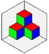
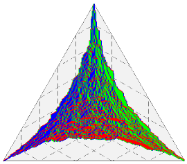
Figure 1: (color online) Upper left: 3d crystal of volume 4. The next elemental cube can be deposited at one of 6 inner corners. Right: Crystal at $t=140$.

The corner growth model admits a dual interpretation as the melting of a three-dimensional cubic crystal by erosion from the corner. There is also a magnetic interpretation in which plus spins are initially assigned to each site inside the corner and minus spins to exterior sites, with the spins endowed with zero-temperature Glauber spin-flip dynamics G63 in a weak negative magnetic field. This dynamics allows only plus spins at inner corners to flip and thus is isomorphic to the corner melting problem. The magnetic interpretation naturally suggests considering the system in zero magnetic field, which results in a growing interface whose characteristic scale grows diffusively rather than ballistically. Other modifications involve changing the initial condition; e.g., depositing the cubes onto a planar substrate (the ‘hypercube stacking model’ step ) leads to a trivial limiting shape but is better-suited to studying non-trivial height fluctuations.

In what follows, we use the language of deposition; most importantly, we allow only deposition events and no evaporation. Growth inside a two-dimensional corner is well understood by mapping the corner growth process onto the one-dimensional asymmetric exclusion process rost ; fluctuations in this limiting shape have also been computed BDJ ; J00 . In three dimensions, the corner growth model can be mapped into an infinite set of coupled exclusion processes in the plane, also known as the ‘zigzag model’ Tamm ; details . Unfortunately, no exact solutions are known for such planar interacting particle processes.

Here we focus on the limiting shape in three (and higher) dimensional corners. Our analysis relies heavily on insights gleaned from the limiting two-dimensional corner interface shape rost . In two dimensions this limiting shape $y(x;t)$ evolves according to the equation of motion Liggett ; spohn ; karma

$$y_{t}=\frac{y_{x}}{y_{x}-1}~{},$$ (1)

from which the interface profile was found to be rost

$$\sqrt{x}+\sqrt{y}=\sqrt{t}\,.$$ (2)

This parabolic shape (2) describes the non-trivial part of the interface where $0\leq x,y\leq t$. Outside this region, the original boundary is undisturbed.

Two properties severely constrain the form of possible evolution equations for growth inside a three-dimensional corner: (a) The governing equation for the interface $z(x,y;t)$ must reduce to the two-dimensional form (1) on the boundaries $x=0$ or $y=0$; (b) The equation must be invariant under the interchange of any coordinate pair.

Analogously to Eq. (1), we seek a three-dimensional evolution equation of the form $z_{t}=F(z_{x},z_{y})$ that involves only first derivatives (higher-order derivatives are asymptotically negligible). The simplest guess is the product $z_{t}=\left[{z_{x}}/({z_{x}-1})\right]\,\left[{z_{y}}/({z_{y}-1})\right]$. This equation reduces to (1) on the boundaries $x=0$, where $z_{x}=-\infty$, and $y=0$, where $z_{y}=-\infty$. The product ansatz is also invariant under the exchange $x\leftrightarrow y$ but not under the exchanges $x\leftrightarrow z$ or $y\leftrightarrow z$ and therefore is wrong.

By extensive trial and error, we found that

$$z_{t}=\frac{z_{x}}{z_{x}-1}\,\frac{z_{y}}{z_{y}-1}\left[1-\frac{1}{z_{x}+z_{y}}\right]$$ (3)

satisfies the necessary coordinate interchange invariances. These constraints severely limit the form of the evolution equation. For example, if we seek a multiplicative correction factor to the product form in (3) as the Laurent series $\sum_{-\infty}^{\infty}\lambda_{n}(z_{x}+z_{y})^{-n}$, coordinate interchange invariance gives $\lambda_{0}=1,\lambda_{1}=-1$, while all other amplitudes vanish details . Thus Eq. (3) is the only invariant choice among the family of evolutionary equations parameterized by $\lambda_{n}$.

We also found one other elemental evolution equation of the form $z_{t}=F(z_{x},z_{y})$ that satisfies coordinate interchange invariance; this form is unique if we again seek corrections as a Laurent series representation. This second solution is obtained by replacing the factor in the square brackets in (3) with $\left[1+({z_{x}z_{y}-z_{x}-z_{y}})^{-1}\right]$. This equation, which can be re-written more elegantly as

$$\frac{1}{z_{t}}=1-\frac{1}{z_{x}}-\frac{1}{z_{y}}\,,$$ (4)

and Eq. (3) are two functionally independent three-dimensional evolution equations that satisfy coordinate interchange invariance. We believe, but cannot prove, that other elemental evolution equations do not exist.

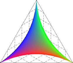
Figure 2: (color online) The interface (5).

Our conjecture is that (3) is the correct evolution equation. Evidence in favor of this statement also comes from the excellent agreement with simulation data. For this comparison, we solve Eq. (3) by the method of characteristics. Starting from an empty corner, we find details that the interface profile admits the following parametric representation (Fig. 2)

$$\frac{x}{t}=A(q,r),\quad\frac{y}{t}=B(q,r),\quad\frac{z}{t}=C(q,r)$$ (5)

where

$$A= \frac{1}{(q-1)^{2}}\frac{r}{r-1}\left[1-\frac{1}{q+r}\right]-\frac{q}{q-1}\frac{r}{r-1}\frac{1}{(q+r)^{2}}~{},$$

$$B= \frac{q}{q-1}\frac{1}{(r-1)^{2}}\left[1-\frac{1}{q+r}\right]-\frac{q}{q-1}\frac{r}{r-1}\frac{1}{(q+r)^{2}}~{},$$

$$C= \frac{q}{q-1}\frac{r}{r-1}\left[1-\frac{1}{q+r}\right]\left[1+\frac{1}{q-1}+\frac{1}{r-1}\right]$$

$$-\frac{q}{q-1}\frac{r}{r-1}\frac{1}{q+r}~{},$$

with $q=z_{x}$, $r=z_{y}$ and $-\infty<q,r\leq 0$. As a consistency check, note that for $r=-\infty$, we have $x/t=(q-1)^{-2}$, $y/t=0$, and $z/t=q^{2}(q-1)^{-2}$. Eliminating $q$, we get $\sqrt{x}+\sqrt{z}=\sqrt{t}$, thereby recovering Eq. (2) for the intersection of the interface (5) with the $y=0$ plane.

It seems impossible to eliminate the parameters $(q,r)$ from Eq. (5) and obtain a closed-form representation of the interface in terms of $x,y,z$ and $t$ as in the two-dimensional case. However, the intersections of the interface (5) with certain planes admit simplified descriptions. For example, for the plane $x=y$, corresponding to $q=r$, we obtain

$$\frac{x}{t}=\frac{1}{2}\frac{z}{t}-\frac{3}{4}\left(\frac{z}{t}\right)^{2/3}+\frac{1}{4}~{},$$ (6)

which agrees well with simulations (Fig. 3).

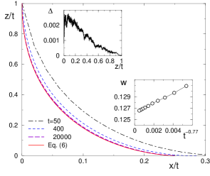
Figure 3: (color online) Scaling plot of the surface profile $z/t$ versus $x/t$ along the diagonal $x=y$ at different times. Upper-left inset: the difference $\Delta$ between the simulated values of the left- and right-sides of (6). Lower-right inset: convergence of the diagonal interface speed versus $t^{-0.77}$.

Two additional tests suggest that the conjectured evolution equation (3) and its solution (5) describe corner growth accurately. Consider first the advance of the interface along the ray $x=y=z$. From (5), the position of this point is given by middle

$$x=y=z=wt,\qquad w=\tfrac{1}{8}\,.$$ (7)

Numerically, we measure $w\approx 0.1261(2)$, which agrees with our prediction $w=0.125$ to within $0.9\%$. As a second test, we compute the total volume $V$ beneath the growing interface at time $t$. Since the linear dimension of the interface grows linearly with time, $V=vt^{3}$. To determine the amplitude $v$, we use the parametric solution (5) and change from the physical variables $(x,y)$ to the parametric coordinates $(q,r)$, from which the amplitude $v$ reduces to the integral

$$v=\int_{-\infty}^{0}\int_{-\infty}^{0}dq\;dr\;C(q,r)\;\frac{\partial(A,B)}{\partial(q,r)}~{}.$$

We compute the Jacobian $\frac{\partial(A,B)}{\partial(q,r)}$ and the integral using Mathematica and find

$$v=\frac{3\pi^{2}}{2^{11}}=0.014457\ldots$$ (8)

Numerically, we measure $v\approx 0.01472(3)$, which is within $1.8\%$ of our prediction.

While Eq. (3) accurately describes the corner interface, small discrepancies between our measurements of the coefficients $w$ and $v$, and their predicted values (7)–(8) persist. The alternative elemental evolution equation (4) leads to the interface profile

$$\sqrt{x}+\sqrt{y}+\sqrt{z}=\sqrt{t}\,,$$ (9)

which is the natural generalization of Eq. (2). The corresponding values $w=\frac{1}{9}$ and $v=\frac{1}{90}$ that arise from this profile substantially disagree with simulation results, suggesting that (4) is wrong.

From the elemental equations (3) and (4), we can also form two distinct one-parameter families of invariant equations details ; an additive family

$$z_{t}=\frac{z_{x}}{z_{x}\!-\!1}\,\frac{z_{y}}{z_{y}\!-\!1}\left[1\!-\!\frac{1+c}{z_{x}+z_{y}}\!-\!\frac{c}{z_{x}z_{y}\!-\!z_{x}\!-\!z_{y}}\right]\!,$$ (10a)

and a multiplicative family

$$z_{t}=\left[\frac{1-\frac{1}{z_{x}+z_{y}}}{\big{(}1-\frac{1}{z_{x}}\big{)}\big{(}1-\frac{1}{z_{y}}\big{)}}\right]^{1+c}\left[1-\frac{1}{z_{x}}-\frac{1}{z_{y}}\right]^{c}\!,$$ (10b)

where for both families the limit $c=0$ reduces to (3) and the limit $c=-1$ reduces to (4). For the multiplicative class of evolution equations (10b), the choice $c\approx 0.074$ provides the best fit for the simulated value of $v$ vel . Similarly, for the additive class of equations, the optimal mixing parameter is $c\approx 0.079$. However, a phenomenon as minimalist as corner interface growth should be described by a simple equation that does not contain an anomalously small mixing parameter. This aesthetic consideration, in conjunction with our numerical results, suggest that Eq. (3) describes corner interface evolution.

The small discrepancies between our simulation results and the predictions that follow from Eq. (3) (see the insets to Fig. 3) suggest that the approach to the asymptotic state is slow. A similarly slow convergence to asymptotic behavior occurs in various well-understood one-dimensional growth models (see e.g. Refs. farnudi ; ferrari ). For example, for 1+1 dimensional corner growth, the intersection of the interface with the $(1,1)$ direction evolves according to BDJ ; J00 ; KK10

$$x(t)=\frac{t}{4}+t^{1/3}\,\xi\,,$$ (11)

where $\xi$ is a stationary random variable with $\langle\xi\rangle>0$. Thus averaging over many realizations gives an effective velocity $w_{\text{eff}}-\frac{1}{4}\sim t^{-2/3}$.

For growth inside a three-dimensional corner, we therefore anticipate that $w_{\text{eff}}-\frac{1}{8}\sim t^{-\alpha}$, with a still-unknown exponent $\alpha$. Very extensive simulations for flat interfaces in 2+1 dimensions indicate that $\alpha$ is close to 0.77 KrugMeakin ; reis ; odor . On the other hand, extrapolation from our simulations for $t\lesssim 20000$ suggests that $\alpha\approx 0.74$. This difference in exponent estimates suggests that $t=20000$ is still outside the long-time regime for growth inside a three-dimensional corner. This slow approach to asymptotic behavior could be the source of the discrepancy between our simulation results and the theoretical prediction (3) for the interface profile.

Our argument for the form of the evolution equation can be generalized to higher dimensions. Applying coordinate interchange invariance and related symmetry considerations, we conjecture that in $d$ dimensions the height $h(x_{1},\ldots,x_{d-1};t)$ satisfies

$$h_{t}=\prod_{1\leq i_{1}<\ldots<i_{p}\leq d-1}\left(1-\frac{1}{h_{i_{1}}+\ldots+h_{i_{p}}}\right)^{(-1)^{p}}$$ (12)

where $h_{i}\equiv\frac{\partial h}{\partial x_{i}}$. These equations are again solvable using the method of characteristics details .

We emphasize that computing the limiting shape — the primary characteristic of the interface — represents only a first step to understanding its properties. One challenging problem, given that interface fluctuations are unknown even for flat interfaces, is to generalize Eq. (11) to account for fluctuations of an interface that grows at a three-dimensional corner. Also of interest are height-height correlations at different locations and different times. In 1+1 dimensions, these correlations decay slowly along the characteristic curves of the evolution equation Borodin ; Ferrari . Whether similar behavior occurs in 2+1 dimensional corner growth is unknown.

Fluctuations of integral characteristics of the interface, such as the crystal volume, may be more tractable and give rise to new phenomena. Consider, for example, the total number of sites of various fixed degrees (number of adjacent vertices). Sites of degree 3, in particular, can be categorized as either inner or outer corners. The number of inner corners grows as $N_{\text{in}}=\frac{dV}{dt}=3vt^{2}$, with $v=3\pi^{2}/2^{11}$ to leading order. One might anticipate the same asymptotic growth for outer corners, but simulations indicate that the latter grows slightly faster details :

$${N_{\text{out}}}/{N_{\text{in}}}\approx 1.04~{}.$$ (13)

Note that in two dimensions $N_{\text{in}}-N_{\text{out}}=1$. For Ising corner growth in three dimensions, $N_{\text{in}}-N_{\text{out}}$ is also positive and grows with time as $t^{1/2}$. This makes the behavior in (13) quite puzzling.

The other major challenges are to generalize from strict corner growth to Ising growth, where adsorption at inner corners and desorption from outer corners occur with equal rates, and to equilibrium interfaces, where the desorption rate exceeds the adsorption rate. The corresponding equilibrium shape has been determined both in two Temp and three dimensions CK_2001 , and its shape fluctuations have also been studied FS . In analogy with the conjectured evolution equations (12) for corner growth, there may also exist an exact generalization of equilibrium limiting shapes Temp ; CK_2001 in higher dimensions.

We thank A. Borodin and H. Spohn for useful correspondence. JO and SR gratefully acknowledge financial support from NSF Grant No. DMR-0906504.

References

- (1) M. Kardar, G. Parisi, and Y.-C. Zhang, Phys. Rev. Lett. 56, 889 (1986).
- (2) T. Halpin-Healey and Y.-C. Zhang, Phys. Rep. 254, 215 (1995).
- (3) T. Kriecherbauer and J. Krug, J. Phys. A 43, 403001 (2010).
- (4) For a review, see I. Corwin, arXiv:1106.1596.
- (5) M. Prähofer and H. Spohn, J. Stat. Phys. 88, 999 (1997).
- (6) R. Rajesh and D. Dhar, Phys. Rev. Lett. 81, 1646 (1998).
- (7) P. Ferrari and A. Borodin, arXiv:0804.3035.
- (8) D. Richardson, Proc. Camb. Phil. Soc. 74, 515 (1973); H. Kesten, Lecture Notes in Math. 1180 125 (Springer, Berlin, 1986).
- (9) R. J. Glauber, J. Math. Phys. 4, 294 (1963).
- (10) M. Plischke, Z. Rácz, and D. Liu, Phys. Rev. B 35, 3485 (1987); B. M. Forrest and L.-H. Tang, Phys. Rev. Lett. 64, 1405 (1990).
- (11) H. Rost, Prob. Theor. Relat. Fields 58, 41 (1981).
- (12) J. Baik, P. A. Deift, and K. Johansson, J. Amer. Math. Soc. 12, 1119 (1999).
- (13) K. Johansson, Commun. Math. Phys. 209, 437 (2000).
- (14) M. Tamm, S. Nechaev, and S. N. Majumdar, J. Phys. A 44, 012002 (2011).
- (15) J. Olejarz, P. L. Krapivsky, S. Redner, and K. Mallick, in preparation.
- (16) T. M. Liggett, Interacting Particle Systems (Springer, New York, 1985).
- (17) H. Spohn, Large Scale Dynamics of Interacting Particles (Springer, Berlin, 1991).
- (18) A. Karma and A. E. Lobkovsky, Phys. Rev. E 71, 036114 (2005).
- (19) Eqeuation (7) follows from (5) by setting . One can also derive (7) directly from (3) without using (5) for the interface shape; it suffices to note that by symmetry at the midpoint.
- (20) Generally for Eq. (10b), one finds , which is best fit to the simulation data by choosing ; similarly for equations from the additive class .
- (21) B. Farnudi and D. D. Vvedensky, Phys. Rev. E 83, 020103(R) (2011).
- (22) P. L. Ferrari and R. Frings, J. Stat. Phys. 144, 1123 (2011).
- (23) J. Krug and P. Meakin, J. Phys. A 23, L987 (1990).
- (24) F. D. A. Aarão Reis, Phys. Rev. E 69, 021610 (2004).
- (25) G. Ódor, B. Liedke, and K.-H. Heinig, Phys. Rev. E 79, 021125 (2009).
- (26) P. Ferrari, J. Stat. Mech. P07022 (2008).
- (27) H. Temperley, Proc. Cambridge Philos. Soc. 48, 683 (1952); A. M. Vershik and S. V. Kerov, Funct. Anal. Appl. 19, 21 (1985); J.-P. Marchand and Ph. A. Martin, J. Stat. Phys. 44, 491 (1986).
- (28) R. Cerf and R. Kenyon, Commun. Math. Phys. 222, 147 (2001); A. Okounkov and N. Reshetikhin, J. Amer. Math. Soc. 16, 581 (2003).
- (29) P. L. Ferrari and H. Spohn, J. Stat. Phys. 113, 1 (2003); P. L. Ferrari, Ph.D. Thesis, Munich University of Technology (2004).