Occurrence of Fermi Pockets without Pseudogap Hypothesis
and Clarification of the Energy Distribution Curves of Angle-Resolved Photoemission Spectroscopy in Underdoped Cuprate Superconductors

Abstract

Central issues in the electronic structure of underdoped cuprate superconductors are to clarify the shape of the Fermi surfaces and the origin of the pseudogap. On the basis of the model proposed by Kamimura and Suwa, which bears important features originating from the interplay of Jahn-Teller physics and Mott physics, the feature of Fermi surfaces in underdoped cuprates is the presence of Fermi pockets constructed from doped holes under the coexistence of a metallic state and a local antiferromagnetic order. Below $T_{\rm c}$, the holes on Fermi pockets form Cooper pairs with d-wave symmetry in the nodal region. In the antinodal region, there are no Fermi surfaces. In this study we calculate the energy distribution curves (EDCs) of angle-resolved photoemission spectroscopy (ARPES) below $T_{\rm c}$. It is shown that the feature of ARPES profiles of underdoped cuprates consists of a coherent peak in the nodal region and real transitions of photoexcited electrons from occupied states below the Fermi level to a free-electron state above the vacuum level in the antinodal region, where the latter transitions form a broad hump. From this feature, the origin of the two distinct gaps observed by ARPES is elucidated without introducing the concept of the pseudogap. Finally, a remark is made on the phase diagram of underdoped cuprates.

1 Introduction

Undoped copper oxide (La₂CuO₄) is an antiferromagnetic Mott insulator, in which an electron correlation plays an important role [1]. Thus, we may say that undoped cuprates are governed by Mott physics. In 1986, Bednorz and Müller discovered high-temperature superconductivity in copper oxides by doping hole carriers into La₂CuO₄ [2]. Their motivation was the consideration that higher $T_{\rm c}$ could be achieved for copper oxide materials by combining Jahn-Teller (JT) active Cu ions with the structural complexity of layer-type perovskite oxides. To investigate the mechanism of high-temperature superconductivity, it is assumed in most models that doped holes itinerate through orbitals extending over a CuO₂ plane in systems consisting of CuO₆ octahedrons elongated by the JT effect. These models are called the “single-component theory”, because the orbitals of hole carriers extend only over a CuO₂ plane.

In 1989, Kamimura and coworkers showed by first-principles calculations that the apical oxygen in CuO₆ octahedrons tends to approach Cu²⁺ ions when Sr²⁺ ions are substituted for La³⁺ ions in La₂CuO₄ in order to gain the attractive electrostatic energy in ionic crystals such as cuprates [3, 4]. As a result, CuO₆ elongated by the JT effect shrinks with hole doping. This deformation against the JT distortion is called the“anti-Jahn-Teller effect” [5]. By this effect, the energy separation between the two kinds of orbital states, which have been split originally by the JT effect, becomes smaller with hole carrier doping. These two states are the a_1g antibonding orbital state $|{\rm a}_{\rm 1g}^{*}\rangle$ and ${\rm b}_{\rm 1g}$ bonding orbital state $|{\rm b}_{\rm 1g}\rangle$. The a${}^{*}_{\rm 1g}$ antibonding orbital state is constructed by a Cu d$z^{2}$ orbital and the six surrounding oxygen p orbitals including apical O p_z-orbitals; the $|{\rm b}_{\rm 1g}\rangle$ orbital is constructed by four in-plane O p_σ orbitals with a small Cu d${}_{x^{2}-y^{2}}$ component parallel to the CuO₂ plane. The spatial extensions of the $|{\rm a}_{\rm 1g}^{*}\rangle$ and $|{\rm b}_{\rm 1g}\rangle$ orbitals, which are perpendicular and parallel to the CuO₂ plane, respectively, are shown in Fig. 1.

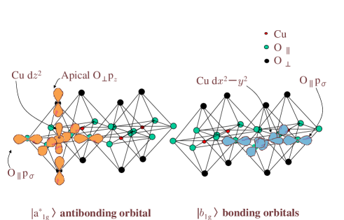
Figure 1: (Color online) Spatial extension of a${}^{*}_{\rm 1g}$ antibonding orbital $|{\rm a}^{*}_{\rm 1g}\rangle$ and b_1g bonding orbital $|{\rm b}_{\rm 1g}\rangle$. a, a${}^{*}_{\rm 1g}$ antibonding orbital $|{\rm a}^{*}_{\rm 1g}\rangle$. b, b_1g bonding orbital $|{\rm b}_{\rm 1g}\rangle$.

By taking account of the anti-Jahn-Teller effect, Kamimura and Suwa reported that one must consider these two kinds of orbital states equally in forming the metallic state of cuprates; they constructed a metallic state coexisting with the local antiferromagnetic (AF) order [6]. This model is called the “Kamimura-Suwa (K-S) model” [7]. Since the anti-Jahn-Teller effect is a central issue of Jahn-Teller physics, we may say that the K-S model bears important features originating from the interplay of Jahn-Teller physics and Mott physics. Since these two kinds of orbitals extend not only over the CuO₂ plane but also along the direction perpendicular to it, the K-S model represents a prototype of a “two-component theory”, in contrast to the single-component theory.

On the basis of the K-S model, Kamimura and Ushio have calculated Fermi surfaces in underdoped La_2-xSr_xCuO₄ (LSCO) [8, 9], and have shown that the coexistence of a metallic state and a local AF order results in the Fermi pockets constructed from doped holes in the nodal region. The appearance of Fermi pockets and small Fermi surfaces in cuprates has recently been reported by various experimental groups [10, 11, 12, 13, 14, 15].

In this study, on the basis of the K-S model, we calculate the energy distribution curves (EDCs) of the angle-resolved photoemission spectroscopy (ARPES) profiles of cuprates below $T_{\rm c}$, and we show that the feature of the calculated ARPES profiles consists of a coherent peak due to the superconducting density of states in the nodal region and the real transitions of electrons from the occupied states below the Fermi level to a free-electron state above the vacuum level in the antinodal region. In particular, we show that the latter transitions form a broad hump in ARPES EDCs in underdoped cuprates.

Concerning the ARPES experiments in underdoped cuprates, Tanaka and coworkers reported very interesting gap features in their observation of ARPES spectra. Their result exhibits a coherent peak in the nodal region and a broad hump in the antinodal region in underdoped Bi2212 samples below $T_{\rm c}$[16]. From the quantitative agreement between the theory and the experiment, we conclude that the observed broad hump corresponds to the photoelectron excitations from the occupied states below the Fermi level to the free-electron state above the vacuum level. In this context, it is concluded that the introduction of the phenomenological idea of the pseudogap is not necessary. Finally, in connection with the finite size of the spin-correlation length in a metallic state, we discuss the finite size effect of a metallic state on the spin-electronic structures of underdoped cuprates, and a new explanation for the phase diagram for underdoped cuprates is proposed.

The organization of the present paper is as follows: At the beginning of §2 we first summarize the essential features of the K-S model, which bears important features originating from the interplay of JT physics and Mott physics. In §3, on the basis of the many-body effects including energy bands obtained from the K-S model, we predict the key features of ARPES EDCs and clarify the origin of the two-gap scenario proposed from the experimental results of Tanaka et al [16]. In §4, we discuss the finite size effects on the Fermi surfaces in cuprates. In connection with the finite size effects, we discuss the possibility of the spatially inhomogeneous distribution of Fermi pocket states and large Fermi surface states. Taking account of the finite size effect, we propose a new interpretation for the phase diagram of underdoped cuprates in §5. We devote §6 to the conclusion and concluding remarks.

2 On the K-S Model

In this section, we summarize the main features of the K-S model [6], emphasizing its important roles in underdoped cuprates due to the interplay of JT physics and Mott physics.

2.1 Key features of the K-S model

The key features of the K-S model are explained in a heuristic way using the picture of a two-story house model shown in Fig. 2. In this figure, the first story of a Cu house is occupied by Cu localized spins, which form the AF order in the spin-correlated region by the superexchange interaction. The second story in the Cu house consists of two floors due to the anti-JT effect; the lower a${}^{*}_{\rm 1g}$ floor and the upper b_1g floor. The second stories of neighboring Cu houses are connected by oxygen rooms, reflecting the hybridization of Cu d and O p orbitals. In the second story, a hole carrier with an up-spin enters the a${}^{*}_{\rm 1g}$ floor of the left-hand Cu house owing to Hund’s coupling with a Cu localized up-spin in the first story (Hund’s coupling triplet) [17, 18], as shown in the leftmost column of the figure. By the transfer interaction marked by a long arrow in the figure, the hole is transferred into the b_1g floor in the neighboring Cu house (second from the left) through the oxygen rooms, where a hole with up-spin forms a spin-singlet state with a localized down-spin in the second Cu house from the left (Zhang-Rice singlet) [19]. The key feature of the K-S model is that the hole carriers in the underdoped regime of LSCO form a metallic state by taking the Hund coupling triplet and the Zhang-Rice singlet alternately in the presence of a local AF order without destroying the AF order, as shown in the figure. From Fig. 2, one may understand that the characteristic feature of the K-S model is the coexistence of the AF order and a normal, metallic (or a superconducting) state in the underdoped regime. This feature of the K-S model (two-component theory) is different from that of the single-component theory.

As seen in Fig. 2, the wave functions of a hole carrier with up and down-spins have the following phase relation:

$$\Psi_{\vec{k}\downarrow}(\vec{r})=\exp(i\vec{k}\cdot\vec{a})\Psi_{\vec{k}\uparrow}(\vec{r}).$$ (1)

Kamimura et al. have shown that this unique phase relation leads to the d-wave superconductivity [20, 21].

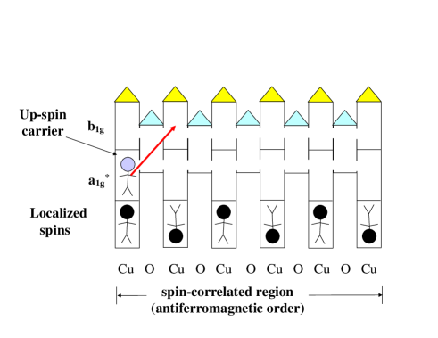
Figure 2: (Color online) Explanation of K-S model using picture of two-story house model.

2.2 Effective Hamiltonian for the K-S model

The following effective Hamiltonian is introduced to describe the K-S model following Kamimura and Suwa [6] (see also ref. 7). It consists of four parts: the one-electron Hamiltonian $H_{\rm sing}$ for the a${}_{\rm 1g}^{\ast}$ and b_1g orbital states, the transfer interaction between neighboring CuO₆ octahedrons $H_{\rm tr}$, the superexchange interaction between the Cu $d_{x^{2}-y^{2}}$ localized spins $H_{\rm AF}$, and the exchange interactions between the spins of dopant holes and $d_{x^{2}-y^{2}}$ localized holes within the same CuO₆ octahedron $H_{\rm ex}$. Thus, we have

$$H = H_{\rm sing}+H_{\rm tr}+H_{\rm AF}+H_{\rm ex}$$ (2)

$$= \sum_{i,m,\sigma}\varepsilon_{m}C_{im\sigma}^{\dagger}C_{im\sigma}$$

$${}+\sum_{\langle i,j\rangle,m,n,\sigma}t_{mn}\left(C_{im\sigma}^{\dagger}C_{jn\sigma}+{\rm h.c.}\right)$$

$${}+J\sum_{\langle i,j\rangle}{\vec{S}}_{i}\cdot{\vec{S}}_{j}+\sum_{i,m}K_{m}\,{\vec{s}}_{i,m}\cdot{\vec{S}}_{i}\ \ ,$$

where $\varepsilon_{m}$ ($m=$ a${}_{\rm 1g}^{\ast}$ or b_1g) represents the one-electron energy of the a${}_{\rm 1g}^{\ast}$ and b_1g orbital states, $C_{im\sigma}^{\dagger}$ and $C_{im\sigma}$ are the creation and annihilation operators of a dopant hole with spin $\sigma$ in the $i$th CuO₆ octahedron, respectively, $t_{mn}$ is the transfer integral of a dopant hole between the $m$-type and $n$-type orbitals of neighboring CuO₆ octahedrons, $J$ is the superexchange interaction between spins ${\vec{S}}_{i}$ and ${\vec{S}}_{j}$ of $d_{x^{2}-y^{2}}$ localized holes in the b${}_{\rm 1g}^{\ast}$ orbital in the nearest-neighbor Cu sites $i$ and $j$ ($J>0$ for AF interaction), and $K_{m}$ is the exchange integral for the exchange interactions between the spin of a dopant hole, ${\vec{s}}_{im}$, and the $d_{x^{2}-y^{2}}$ localized spin ${\vec{S}}_{i}$ in the $i$th CuO₆ octahedron. There are two exchange constants, i.e. $K_{\rm a_{\rm 1g}^{\ast}}$ and $K_{\rm b_{\rm 1g}}$, for the Hund coupling triplet and the Zhang-Rice singlet, respectively, where $K_{\rm a_{\rm 1g}^{\ast}}<0$ and $K_{\rm b_{\rm 1g}}>0$. The appearance of the two kinds of exchange interactions in the fourth term is due to the interplay of Mott physics and JT physics. This is the key feature of the K-S model.

The electron-electron interactions between doped hole carriers are very weak for two reasons: One is the low concentration of hole carriers in the underdoped regime and the other is the wave functions of hole carriers with up and down spins in a CuO₆ octahedron occupying a${}_{\rm 1g}^{\ast}$ and b_1g orbitals, respectively, as seen in eq. (1) and Fig. 1. For these reasons, we have neglected the electron-electron interactions between doped holes in the effective Hamiltonian eq. (2).

By replacing the localized spins ${\vec{S}}_{i}$’s in $H_{\rm ex}$ with their average $\langle{\vec{S}}\rangle$ in the mean-field sense, we can calculate the change in the total energy upon moving a hole from an a${}^{*}_{\rm 1g}$ orbital state in Hund’s coupling spin triplet at Cu site $i$ to an empty b_1g orbital state in the Zhang-Rice spin singlet at the neighboring Cu site $j$. In the first step, the hole moves from Cu site $i$ to infinity. The change in the total energy in the mean field approximation is equal to $\varepsilon_{{\rm a}_{\rm 1g}^{\ast}}+\frac{1}{4}K_{{\rm a}_{\rm 1g}^{\ast}}$. In the second step, the hole moves from infinity to an empty b_1g orbital state at Cu site $j$ to form the Zhang-Rice singlet. The change in the total energy in the second step is equal to $\varepsilon_{\rm b_{\rm 1g}}-\frac{3}{4}K_{\rm b_{\rm 1g}}$. As a result, the change in the total energy by the transfer of the hole from the occupied ${\rm a_{\rm 1g}^{\ast}}$ orbital state at Cu site $i$ to the empty ${\rm b_{\rm 1g}}$ orbital state at Cu site $j$ is

$$\varepsilon_{\rm a_{\rm 1g}^{\ast}}^{\rm~{}eff}-\varepsilon_{\rm b_{\rm 1g}}^{\rm~{}eff}=\varepsilon_{\rm a_{\rm 1g}^{\ast}}+\frac{1}{4}K_{\rm a_{\rm 1g}^{\ast}}-\varepsilon_{\rm b_{\rm 1g}}+\frac{3}{4}K_{\rm b_{\rm 1g}}.$$ (3)

Here, $\varepsilon_{\rm a_{\rm 1g}^{\ast}}^{\rm~{}eff}$ and $\varepsilon_{\rm b_{\rm 1g}}^{\rm~{}eff}$ represent the effective one-electron energies of the a${}_{\rm 1g}^{\ast}$ and b_1g orbital states including the exchange interaction term $H_{\rm ex}$, respectively. Thus, the energy difference $(\varepsilon_{\rm a_{\rm 1g}^{\ast}}^{\rm~{}eff}-\varepsilon_{\rm b_{\rm 1g}}^{\rm~{}eff})$ corresponds to the energy difference between the ${\rm a_{\rm 1g}^{\ast}}$ and ${\rm b_{\rm 1g}}$ floors in the second story in Fig. 2.

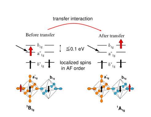
Figure 3: (Color online) Simple explanation for coexistence of metallic state and local AF order in two-component theory (a${}^{*}_{\rm 1g}$ and b_1g orbital states), by taking neighboring Cu sites $i$ to $j$ as an example, where localized spins are in antibonding b${}^{\ast}_{\rm 1g}$ orbitals. Schematic pictures of Hund’s coupling triplet ³B_1g and Zhang-Rice singlet ¹A_1g are also shown at the bottom. The energy in this figure is taken as the hole energy.

Now, let us estimate the energy difference $\varepsilon_{\rm a_{\rm 1g}^{\ast}}^{\rm~{}eff}$ - $\varepsilon_{\rm b_{\rm 1g}}^{\rm~{}eff}$ using the values of the parameters in the effective Hamiltonian eq. (2). The values of the parameters in Hamiltonian eq. (2) have been determined in the case of LSCO in ref. 6 (see also ref. 7). They are $J=0.1$, $K_{\rm a_{\rm 1g}^{\ast}}=-2.0$, $K_{\rm b_{\rm 1g}}=4.0$, $t_{\rm a_{\rm 1g}^{\ast}a_{\rm 1g}^{\ast}}=0.2$, $t_{\rm b_{\rm 1g}b_{\rm 1g}}=0.4$, $t_{\rm a_{\rm 1g}^{\ast}b_{\rm 1g}}=\sqrt{t_{\rm a_{\rm 1g}^{\ast}a_{\rm 1g}^{\ast}}t_{\rm b_{\rm 1g}b_{\rm 1g}}}\sim 0.28$, $\varepsilon_{\rm a_{\rm 1g}^{\ast}}=0$, and $\varepsilon_{\rm b_{\rm 1g}}=2.6$ in units of eV, where $K_{\rm a_{\rm 1g}^{\ast}}$ and $K_{\rm b_{\rm 1g}}$ are taken from first-principles cluster calculations for a CuO₆ octahedron in LSCO [17, 18], and the $t_{mn}$ are obtained by band structure calculation [3, 4]. The difference in one-electron energy between the a${}_{\rm 1g}^{\ast}$ and b_1g orbital states in a CuO₆ octahedron for a certain $x$ has been determined so as to reproduce the difference in the lowest state energy between Hund’s coupling spin-triplet state and the Zhang-Rice spin-singlet state for the same $x$ in LSCO calculated by Multi-Configuration Self-Consistent Field (MCSCF) cluster calculations which include the anti-JT effect [6].

Thus, the calculated $\varepsilon_{\rm a_{\rm 1g}^{\ast}}^{\rm~{}eff}$ - $\varepsilon_{\rm b_{\rm 1g}}^{\rm~{}eff}$ is 0.1 eV in the case of the optimum doping ($x=0.15$). Then, by introducing the transfer interaction of $t_{\rm a_{\rm 1g}^{\ast}b_{\rm 1g}}=0.28$ eV, a coherent metallic state in the normal phase is obtained in the presence of the local AF order for the underdoped regime. This situation is schematically shown in Fig. 3.

2.3 Features of the many-body effect including energy bands and Fermi surfaces of underdoped LSCO coexisting with the AF order

In the previous subsection, we have shown that the effective Hamiltonian eq. (2) for the K-S model can lead to a unique metallic state in the normal phase, which results in the coexistence of a superconducting state and an AF order below $T_{\rm c}$. In 1994, Kamimura and Ushio calculated the energy bands and Fermi surfaces of underdoped LSCO in the normal phase on the basis of the effective Hamiltonian eq. (2), by treating the fourth term $H_{\rm ex}$ in the effective Hamiltonian eq. (2) by the mean-field approximation, that is, by replacing the localized spins ${\vec{S}}_{i}$’s with their average $\langle{\vec{S}}\rangle$ [8, 9]. Thus, the effect of the localized spin system was dealt with as an effective magnetic field acting on hole carriers. As a result, Kamimura and Ushio separated the localized hole-spin system in the AF order and the hole carrier system from each other, and calculated the “one-electron type” energy band for a carrier system assuming a periodic AF order. Here, “one-electron type” means the inclusion of many-body effects in the energy bands. That is, the effect of the exchange interactions between carriers and localized spins is included in the sense of the mean field approximation.

In Fig. 4, the calculated many-body effect including energy band structure for up-spin (or down-spin) doped holes in LSCO is shown for various values of the wave vector $\vec{k}$ and symmetry points in the AF Brillouin zone, where the AF Brillouin zone is adopted because of the coexistence of a metallic state and the AF order; it is shown on the left side of the figure. Here, note that the energy in this figure is taken as the electron energy but not as the hole energy. Furthermore, the Hubbard bands for localized b${}^{\ast}_{\rm 1g}$ holes, which contribute to the local AF order, are separated from this figure and do not appear in this figure.

In undoped La₂CuO₄, all the energy bands in Fig. 4 are fully occupied by electrons so that La₂CuO₄ is an AF Mott insulator, consistent with experimental results. In this respect, the present effective energy band structure is completely different from the structure of ordinary LDA energy bands [22, 23]. When Sr is doped, holes begin to occupy the top of the highest band in Fig. 4 marked by #1 at the $\Delta$ point, which corresponds to $(\pi/2a,\pi/2a,0)$ in the AF Brillouin zone. At the onset concentration of superconductivity, the Fermi level is located slightly below the top of the #1 band at $\Delta$, which is slightly higher than the G₁ point. Here, the G₁ point in the AF Brillouin zone lies at $(\pi/a,0,0)$ and corresponds to a saddle point of the van Hove singularity.

Figure 4: Many-body effect including band structure [8, 9] for up-spin (or down-spin) dopant holes in underdoped LSCO above $T_{\rm c}$. The highest occupied band is marked by the #1 band (right) and the AF Brillouin zone (left). The $\Delta$ point corresponds to $(\pi/2a,\pi/2a,0)$, while the G₁ point corresponds to $(\pi/a,0,0)$, at which a saddle-point singularity appears.

Figure 5: (Color online) Fermi surface (FS) for up-spin (or down-spin) dopant holes in underdoped LSCO above $T_{\rm c}$. The FS consists of four Fermi pockets around the $\Delta$ point, $(\pi/2a,\pi/2a,0)$, and the other three equivalent points (the nodal region) in momentum space. The figure shows the two-dimensionally projected Fermi pockets. The point A represents one of the electronic states.

On the basis of the calculated band structure shown in Fig. 4, Kamimura and Ushio [8, 9] calculated the Fermi surface (FS) for the underdoped regime of LSCO. The calculated FS in the underdoped regime is composed of four Fermi pockets of extremely flat tubes. The projected two-dimensional (2D) picture of the four Fermi pockets around the $\Delta$ point, $(\pi/2a,\pi/2a)$ and the other three equivalent points in the momentum space is shown in the antiferromagnetic Brillouin zone in Fig. 5. The total volume of the four Fermi pockets is proportional to the concentration of the doped hole carriers. Thus, the feature of Fermi pockets constructed from the doped holes shown in Fig. 5 is consistent with Luttinger’s theorem in the presence of AF order [24].

In 1996 and 1997, respectively, Mason et al. [25] and Yamada et al. [26] independently reported the magnetic coherence effects on the metallic and superconducting states in underdoped LSCO, determined by neutron inelastic scattering measurements. Since then, a number of papers suggesting the coexistence of local AF order and superconductivity in cuprates as a result of neutron and NMR experiments have been published [27, 28, 29, 30, 31, 32].

The Fermi surface structure in Fig. 5 is completely different from that of the single-component theory, in which the FS is large. Recently, Meng et al. have reported the existence of the Fermi pocket structure in the ARPES measurements of underdoped Bi₂Sr_2-xLa_xCuO_6+δ (La-Bi2201) [10]. Their results are clear experimental evidence of our Fermi pocket structure for underdoped LSCO predicted in 1994 [8].

In 1997, Anisimov et al. calculated the energy band structure of the ordered alloy La₂Li_0.5Cu_0.5O₄ by the LDA+U method [33], and they showed that a fairly modest reduction in the apical Cu-O bond length is sufficient to stabilize Hund’s coupling spin triplet state with dopant holes in both b_1g and a${}^{\ast}_{\rm 1g}$ orbitals. Their calculated result supports the K-S model.

3 Calculation of ARPES Spectra Based on the K-S Model and the Conclusion of the Absence of a Pseudogap

Recently, considerable attention has been paid to the phenomenological idea of the pseudogap. When a portion of the Fermi surface in cuprates was not observed in the ARPES experiments, the idea of the pseudogap was proposed as a type of gap for truncating the FS in a single-particle spectrum [34, 35]. The disconnected segments of the FS are called the “Fermi arc” [13, 35, 36]. Further ARPES experiments showed that such a pseudogap develops below a temperature denoted $T^{*}$, which depends on the hole concentration $x$ in the underdoped regime of cuprates; thus, we write $T^{*}(x)$ hereafter. $T^{*}(x)$ decreases with increasing hole concentration $x$ and disappears at a certain concentration $x_{\rm o}$ in the overdoped region [37]. In this section, on the basis of the K-S model, we clarify the origins of the pseudogap and $T^{*}(x)$.

3.1 Calculation of the photoemission intensity and clarification of the origin of the observed two distinct gaps

Below $T_{\rm c}$, the hole carriers in the Fermi pockets shown in Fig.5 form Cooper pairs, contributing to the formation of a superconducting state, and a superconducting gap appears across the Fermi level. This feature is consistent with Uemura et al.’s plot [38]. In Fig. 6(a), the d-wave node below $T_{\rm c}$ predicted by the K-S model [20, 21] is schematically shown as dots, and the d-wave superconducting density of states is schematically shown in Fig. 6(b). Here, note that the AF order still coexists with a superconducting state below $T_{\rm c}$ so that we can use the same AF Brillouin zone, as shown in Fig. 6.

Figure 6: (Color online) Sketch of d-wave superconductivity in K-S model below $T_{\rm c}$. (a) Change of Fermi pockets in nodal region to d-wave nodes below $T_{\rm c}$. (b) d-Wave superconducting density of states.

On the other hand, in the antinodal region, the states occupied by electrons that do not participate in the formation of superconductivity still exist below $T_{\rm c}$. As an example of such states, the state A is shown in Fig. 6(a), and the state corresponding to A above $T_{\rm c}$ is also shown in Fig. 5. Then, real transitions of electrons from the occupied states, say, the state A, below the Fermi level $\varepsilon_{\rm F}$ in the #1 energy band in Fig. 4 to a free-electron state above the vacuum level occur by photoexcitation both above and below $T_{\rm c}$ around the G₁ point $(\pi/a,0,0)$ and other equivalent points in momentum space. These transitions appear in the antinodal region in momentum space.

Such a transition is shown in Fig. 7 [39]. Let us consider the case in which an electron in the occupied state A with energy $\varepsilon_{i}$ and momentum ${\vec{k}}_{i}$ in the $\#1$ energy band below $\varepsilon_{\rm F}$ is excited to a free-electron state with the bottom of the energy dispersion at $(\varepsilon_{\rm F}-\varepsilon_{\rm o})$ in a crystal by a photon with energy $h\nu$, where we use the suffix $i$ to emphasize the initial state of the transition in the crystal. Thus, the final state of the transition with energy $\varepsilon_{\rm f}$ in the crystal is expressed as

$$\varepsilon_{\rm f}=\frac{\hbar^{2}}{2m}(k_{\parallel}^{2}+k_{\perp}^{2})+\varepsilon_{\rm F}-\varepsilon_{\rm o},$$ (4)

where $k_{\parallel}$ and $k_{\perp}$ are the momenta of the photoexcited electron parallel and perpendicular to the crystal surface, respectively. As shown in Fig. 7, the energy conservation for this excitation process from the initial state $|{i\rangle}$ to the final state $|{f\rangle}$ in the crystal is expressed as $h\nu=\varepsilon_{\rm f}-\varepsilon_{\rm i}$ for a photon of energy $h\nu$.

Figure 7: (Color online) Energetics of photoemission process.

When an electron is ejected into the vacuum level of the crystal by a photon with energy ${\hbar\nu}$, it acquires kinetic energy. Through ARPES experiments, we measure the kinetic energy of photoelectrons emitted in vacuum. We define the kinetic energy of such photoelectrons emitted in vacuum as $\varepsilon_{\rm kin}$, where $\varepsilon_{\rm kin}=(\hbar^{2}/2m)(K_{\parallel}^{2}+K_{\perp}^{2})$.

On the other hand, the binding energy of the electron in the initial state, $E_{\rm B}$, is introduced as a new variable instead of $\varepsilon(k_{\rm i})$. $E_{\rm B}$ is defined as

$$E_{\rm B}=-\varepsilon(k_{\rm i})+\varepsilon_{\rm F}.$$ (5)

The following equation also holds for $\varepsilon_{\rm f}$:

$$\varepsilon_{\rm f}=\varepsilon_{\rm kin}+W+\varepsilon_{\rm F},$$ (6)

where $W$ is the work function of the crystal (see Fig. 7).

In the ARPES experiment, when a photoelectron is emitted from a crystal in vacuum through a surface, it is assumed that the momentum parallel to the surface is conserved: $k_{\parallel}=K_{\parallel}$. Now, note that the $\#1$ band in Fig. 4 has been calculated by the mean field approximation for the fourth term in the Hamiltonian (2). The important consequence of this approximation is that, having taken into account the strong spin exchange interaction in the mean field approximation, the probability of removing an electron in the state with momentum $\vec{k}_{\rm i}$ and energy $\varepsilon_{\rm i}$ in the $\#1$ energy band to the free-electron state in vacuum can be treated in a framework similar to that for single-particle photoexcitation.

As a result, the EDCs in the ARPES experiments corresponding to the transition from the occupied states in the many-body effect including energy band in Fig. 4 to the free-electron band can be calculated using the following formula for the photoemission intensity $I(\vec{k},\omega)$:

$$I(\vec{k},\omega)=\left|M_{\vec{k}}\right|^{2}A(\vec{k},\omega)\rho_{\rm f}(\varepsilon_{\rm kin}).$$ (7)

Here, $A(\vec{k},\omega)$ is the spectral function that gives the probability of removing or adding an electron at $(\vec{k},\omega)$, where $\omega$ is the electron energy relative to the Fermi level. It is related to the imaginary part of the one-electron Green’s function; $A(\vec{k},\omega)=-(1/{\pi}){\rm Im}G(\vec{k}.\omega)$. Furthermore, $\rho_{\rm f}(\omega)$ is the density of final states and $\left|M_{\vec{k}}\right|^{2}$ is the squared one-electron transition matrix element[40]. It is clear from Fig. 7 that $A(\vec{k},\omega)$ gives the highest probability when $\hbar\omega$ is equal to $(h\nu-\varepsilon_{\rm kin}-W)$, where $h\nu$ = $\varepsilon(k_{\rm f})$ - $\varepsilon(k_{\rm i})$.

By taking account of the lifetime effects due to the finite size of a metallic state, the deviation from the mean field approximation, and other factors, the spectral function $A(\vec{k},\omega)$ is given by

$$A(\vec{k},\omega)=(1/\pi)\frac{\delta}{[\hbar\omega-(\varepsilon_{\rm F}-\varepsilon(\vec{k_{\rm i})})]^{2}+\delta^{2}},$$ (8)

where $\delta$ denotes the lifetime effects, and the momentum dependence in $\varepsilon_{\rm i}$ is expressed as $\varepsilon(\vec{k_{\rm i}})$ explicitly.

The density of final states $\rho_{\rm f}(\varepsilon_{\rm kin})$ in the EDCs is defined from the dispersion of the momentum of a photoexcited electron perpendicular to the crystal surface in the crystal, $k_{\perp}$, as,

$$\rho_{\rm f}(\varepsilon_{\rm kin})=\left|\frac{{\rm d}k_{\perp}}{{\rm d}\varepsilon_{\rm kin}}\right|.$$ (9)

Using eqs. (4) and (6) with the conservation of momentum of a photoexcited electron parallel to the crystal surface, $k_{\parallel}$ = $K_{\parallel}$, the density of final states is obtained as,

$$\rho_{\rm f}(\varepsilon_{\rm kin})=\frac{1}{2\,\sqrt{(\hbar^{2}/2m)\left(\varepsilon_{\rm kin}+V-(\hbar^{2}/2m)k_{\parallel}^{2}\right)}},$$ (10)

where $V$ = $W$ + $\varepsilon_{\rm o}$ is the inner potential. This result agrees with the result derived by Mizokawa [41].

Since much of the ARPES EDC data is expressed as a function of the binding energy $E_{\rm B}$, we express eqs. (8) and (10) in terms of $E_{\rm B}$. For this purpose, we first insert eq. (5) into eq. (8), and simultaneously replace $\hbar\omega$ in eq. (8) by $(h\nu-\varepsilon_{\rm kin}-W)$. As a result, eq. (8) can be written as,

$$A(\vec{k},\omega)=(1/\pi)\frac{\delta}{[(h\nu-\varepsilon_{\rm kin}-W)-E_{\rm B}]^{2}+\delta^{2}}.$$ (11)

Furthermore, using the expression for the inner potential, $V$ = $W$ + $\varepsilon_{\rm o}$, and the energy conservation relation in Fig.7 given as

$$h\nu=\varepsilon_{\rm kin}+W+E_{\rm B},$$ (12)

eq. (10) can be expressed as

$$\rho_{\rm f}(\varepsilon_{\rm kin})=\frac{1}{2\,\sqrt{(\hbar^{2}/2m)\left(h\nu-E_{\rm B}+\varepsilon_{\rm o}-(\hbar^{2}/2m)k_{i\parallel}^{2}\right)}},$$ (13)

where $k_{i\parallel}$ is the component of ${\vec{k}}_{i}$ parallel to the crystal surface.

Using eqs. (7), (12), and (13), we have calculated the photoemission intensity $I(\vec{k},\omega)$ as a function of $E_{\rm B}(\vec{k_{\rm i}})$. In performing the numerical calculations, we have considered that the photon energy ($h\nu$) range in synchrotron radiation experiments is 10 to 100 eV and the kinetic energy range of the photoelectron is also 10 to 100 eV [42]. Since the width of the energy dispersion of the $\#1$ energy band in Fig. 4(a) is about 1 eV, we notice that the $E_{\rm B}$ range is up to 1 eV. For $\delta$, whose inverse gives a measure of the lifetime broadening in the $\#1$ band, we assume 100 meV on the basis of the discussion in the subsequent section.

In this context, we choose 15 eV for $h\nu$, 10 eV for $\varepsilon_{\rm kin}$, 3.5 eV for W [43], and 4.5 eV for the inner potential $V$ = $\varepsilon_{\rm o}$ + $W$ in the present numerical calculations. As regards $\hbar^{2}k_{i\parallel}^{2}/2m$, we choose the center of the antinodal region, i.e., the $G_{1}$ point or the edge of the AF Brillouin zone in Fig. 4, for the $i$th point, because the antinodal region is narrow around the $G_{1}$ point, so that $\hbar^{2}k_{i\parallel}^{2}/2m$ does not change much upon varying the $i$th point. By adopting the empty lattice test for the free-electron energy bands, we estimate $\hbar^{2}k_{i\parallel}^{2}/2m$ to be 3 eV for $i$ = $G_{1}$.

The calculated $I(\vec{k},\omega)$ with the values of the above parameters is shown as a function of $E_{B}$ in Fig. 8(a). Since $\varepsilon_{\rm kin}$ is very large, a divergent point in the density of final states $\rho_{\rm f}(\omega)$ appears at a large $E_{\rm B}$. Thus, the photoemission intensity $I(\vec{k},\omega)$ shows a feature of a broad hump, reflecting a peak in the spectral function $A(\vec{k},\omega)$ given by eq. (11), as seen in Fig. 8(a). This trend is consistent with the experimental results of the ARPES spectra of underdoped Bi2212 samples below $T_{\rm c}$ in the antinodal region by Tanaka et al. [16], although the shape of the broad hump is slightly different.

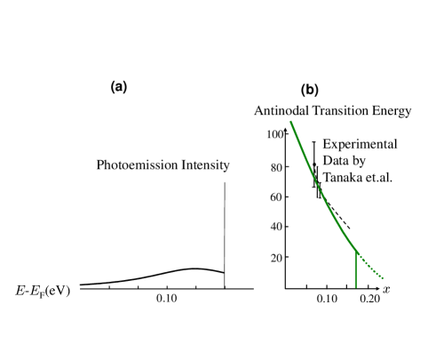
Figure 8: (Color online) Calculated ARPES spectra of LSCO and their comparison with experimental results of Bi2212. (a) Calculated photoemission intensity as a function of binding energy $E_{B}(=E-E_{\rm F})$. (b) Calculated energy difference $|\varepsilon({\rm G}_{1})-\varepsilon_{\rm F}(x)|$ (antinodal transition energy) as a function of hole concentration $x$ at $T=0$K. Experimental results of Tanaka et al. [16] are shown by dots.

From the ARPES spectra in the nodal region shown in Fig. 6(b), which was predicted from the d-wave superconductivity due to the K-S model, [20] and those in the antinodal region shown in Fig. 8(a), we can conclude that the features of ARPES spectra below $T_{\rm c}$ are theoretically as follows: ARPES spectra consist of a coherent peak due to the superconducting density of states that appears in the nodal region around the $\Delta$ point and a broad hump that appears in the antinodal region, which corresponds to the real transition of electrons from the occupied states below the Fermi level $\varepsilon_{\rm F}$ to a free-electron state above the vacuum level. These theoretical results of ARPES EDCs are similar to the experimental ones reported by Tanaka et al. for Bi2212 [16], where the experimental results revealed two distinct energy gaps in the nodal and antinodal regions exhibiting different doping dependences. Thus, we designate the broad hump in the antinodal region as an “antinodal transition”, where $\varepsilon_{\rm F}$ varies with the hole concentration $x$, so that we write $\varepsilon_{\rm F}(x)$ hereafter.

Furthermore, Tanaka et al. reported the doping dependence of the position of the hump, which is determined from the second derivative of the spectra in the antinodal region around the $G_{1}$ point for the three underdoped samples in Bi2212. We compare this experimental result of Bi2212 with the calculated doping dependence of the binding energies $E_{B}$ at the $G_{1}$ point for LSCO, which correspond to the energy difference $|\varepsilon({\rm G}_{1})-\varepsilon_{\rm F}(x)|$. We call this energy difference the “antinodal transition energy”.

Since the shape of the density of states (DOS) for the highest conduction band does not depend on the type of cuprate material, we can compare in Fig. 8(b) the calculated doping dependence of the antinodal transition energy for LSCO (solid lines) with the experimental results of the antinodal gap of Bi2212 in ref.16, which are shown as dots in the figure. As seen in Fig. 8(b), the agreement between the theory and the experiment is remarkably good. From this quantitative agreement, we can conclude that among the observed two gaps below $T_{\rm c}$, the gap associated with the antinodal regime corresponds to the real transitions of electrons from the occupied states below the Fermi level to a free-electron state above the vacuum level, while the other gap associated with the near-nodal regime corresponds to the superconducting gap created on Fermi pockets. From the excellent agreement between the present theoretical results and the experimental results of Tanaka et al., we can conclude that the real transitions of electrons from occupied states below the Fermi level to a free-electron state above the vacuum level by photoexcitation appear in the antinodal region in underdoped cuprates so that the introduction of a pseudogap is not necessary.

Recently, Yang et al. [44] have suggested from their ARPES experiments on Bi2212 that the opening of a symmetric gap related to superconductivity occurs only in the antinodal region and that the pseudogap reflects the formation of preformed pairs, in contrast to the ARPES experimental results reported by Tanaka et al [16]. In the present theory, we have clearly shown in Figs. 6 and 8 that, in the ARPES experiments, a peak related to superconductivity appears only in the nodal region and that the spectra in the antinodal region correspond to photoexcitations from occupied states below $\varepsilon_{\rm F}$ to a free-electron state above the vacuum level. If the antinodal region in ref. 44 is the region around the ${\rm G}_{1}$ point in the present paper, their suggestion is in disagreement with our theoretical results. Finally, we should remark that any proposed theory must explain both the doping and temperature dependences of ARPES spectra in the underdoped regime consistently. From this standpoint, we will investigate the temperature dependence of the calculated broad hump in ARPES EDCs theoretically in the next subsection.

3.2 Physical meaning of $T^{*}(x)$ and the temperature dependence of ARPES spectra

To calculate the temperature dependence of the antinodal transition energy, first we would like to clarify the physical meaning of $T^{*}(x)$. When a hole concentration $x$ is fixed at a certain value in the underdoped region and the temperature increases beyond $T_{\rm c}$, in the normal phase, the local AF order constructed by superexchange interaction in a CuO₂ plane is destroyed by thermal agitation, and thus a phase showing the coexistence of a metallic state with the Fermi pockets and the local AF order diminishes gradually. As a result, an electronic phase consisting of a large FS without the AF order is mixed with a phase of the K-S model. Finally, at a certain temperature, a uniform phase consisting of the electronic phase consisting of a large FS without the AF order will appear in the underdoped regime. This temperature is defined as $T^{*}(x)$. Thus, the phase of the Fermi pockets coexisting with the local AF order in the K-S model holds only below $T^{*}(x)$. We designate the phase of the Fermi pockets in the K-S model as the “small FS” phase and the electronic phase consisting of a large FS without the AF order as the “large FS” phase. Hereafter, the former and latter are abbreviated as the SF and LF phases, respectively. In this context, one may consider that a phase below $T^{*}(x)$ is a mixed phase of the SF and LF phases in the underdoped regime; thus, $T^{*}(x)$ represents a crossover from the mixed phase to the LF phase.

To calculate $T^{*}(x)$ on the basis of the K-S model, one must take account of the effect of thermal agitation in the system of Cu localized spins in the AF order (the first story in Fig. 2). However, such calculation is possible only for a finite system, as Hamada and coworkers have shown [45, 46]. In this context, we calculate $T^{*}(x)$ approximately, neglecting the effect of thermal agitation in the system of Cu localized spins.

For this purpose, let us introduce a quantity that defines the difference between the free energies of pure LF and SF phases:

$$\Delta F(T,x) \equiv F_{\rm LF}(T,x)-F_{\rm SF}(T,x),$$ (14)

where $F_{\rm LF}(T,x)$ and $F_{\rm SF}(T,x)$ are the free energies of the LF and SF phases, respectively. Here the free energy $F(T,x)$ is defined as

$$F(T,x) = E(T,x)-TS(T,x),$$ (15)

where $E(T,x)$ and $S(T,x)$ are the internal energy and entropy of each phase, respectively. These quantities are calculated from

$$E(T,x) = \int^{\infty}_{-\infty}\varepsilon\rho(\varepsilon)f(\varepsilon,\mu(x)){\rm d}\varepsilon,$$ (16)

and

$$S(T,x) = -k_{\rm B}\int^{\infty}_{-\infty}\Bigl{[}f(\varepsilon,\mu(x))\ln f(\varepsilon,\mu(x))$$ (17)

$${}+\bigl{\{}1-f(\varepsilon,\mu(x))\bigr{\}}\ln\bigl{\{}1-f(\varepsilon,\mu(x))\bigr{\}}\Bigl{]}~{}$$

$$~{}~{}~{}~{}~{}~{}~{}~{}~{}~{}~{}~{}~{}~{}~{}~{}~{}~{}~{}~{}~{}~{}~{}~{}~{}~{}~{}~{}~{}~{}~{}~{}~{}~{}~{}~{}~{}~{}\rho(\varepsilon)~{}d\varepsilon\,,$$

where $\mu(x)$ is the chemical potential of each phase, $\rho$($\varepsilon$) is the DOS for each phase, and $f(\varepsilon,\mu(x))$ is the Fermi distribution function at energy $\varepsilon$ and chemical potential $\mu(x)$. Then, $\tilde{T}^{*}(x)$ is defined by

$$\Delta F(\tilde{T}^{*}(x),x)=0.$$ (18)

Figure 9: (Color online) (a) Calculated temperature dependence of antinodal transition energy for $x$ = 0.05, 0.1, and 0.15. Experimental data obtained by Norman et al. [47] (triangles) and Lee et al. [48] (squares) are shown. (b) Calculated result of $\tilde{T}^{*}(x)$ as a function of the hole concentration $x$

Kamimura et al. calculated the electronic entropies for the SF and LF phases of LSCO [7]. According to their results, the difference in electronic entropy between the SF and LF phases increases with increasing hole concentration $x$ in the underdoped regime. Using this result, we have calculated $\tilde{T}^{*}(x)$ from eq. (18) as a function of $x$, instead of $T^{*}(x)$. In doing so, we have introduced two parameters, $\tilde{T}^{*}(x=0.05)$ and $x_{\rm o}$, where $x_{\rm o}$ is the critical concentration that satisfies $\tilde{T}^{*}(x_{\rm o})$=0. Here, $\tilde{T}^{*}(x=0.05)$ represents a quantity related to the energy difference between the phase of the doped AF insulator and the LF phase at the onset concentration of the metal- insulator transition ($x=0.05$). $\tilde{T}^{*}(x=0.05)$ is chosen to be 300K. On the other hand, the physical meaning of $\tilde{T}^{*}(x_{\rm o})=0$ can be explained as follows: When the hole concentration exceeds the optimum doping level ($x$ = 0.15) for LSCO and enters a slightly overdoped region, the local AF order via superexchange interaction in a CuO₂ plane is destroyed by an excess of hole carriers. Thus, the K-S model does not hold at a certain concentration $x_{\rm o}$ in the overdoped region, and hence the small FS in the K-S model changes to a large FS. Thus, $\tilde{T}^{*}(x)$ vanishes at $x_{\rm o}$. From the analysis of various experimental results, we choose $x_{\rm o}$ = 0.17 for LSCO [49, 50]. The calculated result of $\tilde{T}^{*}(x)$ with $\tilde{T}^{*}(x=0.05)$ = 300K and $x_{\rm o}$ = 0.17 is shown as a function of $x$ in Fig. 9b.

From the present result, we can say that the area below $\tilde{T}^{*}(x)$ in the underdoped regime represents the region in which the normal (metallic) phase above $T_{\rm c}$ and the superconducting phase below $T_{\rm c}$ coexist with the local AF order. In a real system, a region of a mixed phase consisting of the SF and LF phases appears between $\tilde{T}^{*}(x)$ and $T^{*}(x)$ owing to the dynamical interaction of the fourth term in the effective Hamiltonian (2). Thus, $T^{*}(x)$ always appears above $\tilde{T}^{*}(x)$ [51].

Under this circumstance, it is clear that the antinodal transition energy defined by $|\varepsilon({\rm G}_{1})-\varepsilon_{\rm F}(x)|$ appears at temperatures below $T^{*}(x)$ and vanishes at $T^{*}(x)$. By using $\tilde{T}^{*}(x)$ instead of $T^{*}(x)$, we calculate the temperature dependence of the antinodal transition energy using eqs. (14)-(17). The calculated results for three concentrations, i.e., $x$ = 0.05, 0.10, and 0.15, of LSCO in the underdoped-to-optimallydoped region are shown in Fig. 9(a) as functions of temperature, where $\tilde{T}^{*}(0.05)=300$K is used. As seen in the figure, the antinodal transition energy increases slightly with temperature up to $\tilde{T}^{*}(x)$ and vanishes suddenly at $\tilde{T}^{*}(x)$. These calculated results are compared with the experimental results of the underdoped sample of Bi2212 in refs. 47 and 48, which are indicated by triangles and squares, respectively, in Fig. 9(a). As seen in the figure, the agreement between the theory and the experiment is remarkably good, although the present theoretical treatment is not rigorous in the sense that, in the calculation of $F_{\rm SF}(T,x)$, the dynamical interplay of a metallic state (the second story in Fig. 2) and Cu localized spins in the AF order (the first story) is not taken into account.

4 Spatially Inhomogeneous Distribution of Fermi Pocket States and Large Fermi Surface States due to the Finite Size Effects

4.1 Finite size effects of metallic state on Fermi surface

According to the results of neutron inelastic scattering experiments by Mason et al. [25] and Yamada et al. [26], the AF spin-correlation length $\lambda_{s}$ in the underdoped region of LSCO is finite. In the underdoped regime of LSCO, it increases as the Sr concentration increases from $x=0.05$ in LSCO, the onset of superconductivity, and reaches about 50Å or more at the optimum doping level ($x=0.15$). In this subsection, we discuss the effects of the finite size of the AF spin-correlation length on the structure of the Fermi pockets shown in Fig. 5. According to the K-S model in Fig. 2, in the spin-correlated region a doped hole in the underdoped regime of LSCO can itinerate coherently by taking the a${}^{*}_{\rm 1g}$ and b_1g orbitals alternately in the presence of the local AF order without destroying the AF order.

In the case of a finite spin-correlated region, one may think that there are frustrated spins at the boundary between the spin-correlated region of the AF order and the region of the “resonating valence bond” (RVB) state proposed by Anderson [1] without hole carriers. Here, the frustrated spins mean that the localized spins at the boundary are not in the AF order, but directed parallel to each other. Suppose that one of the frustrated spins in a parallel direction at the boundary changes its direction from parallel to antiparallel by the fluctuation effect in the 2D Heisenberg AF spin system during the time of $\tau_{s}$ defined by $\tau_{s}\equiv\hbar/J$, where $J$ is the superexchange interaction ($\sim$0.1 eV). At the time of $\tau_{s}$, on the other hand, hole carriers at the Fermi level can move with the Fermi velocity inside the spin-correlated region of the AF order. The traveling time of a doped hole at the Fermi level over an area of the spin-correlation length is given by $\tau_{\rm F}\equiv\lambda_{s}/v_{\rm F}$, where $v_{\rm F}$ is the Fermi velocity of a doped hole at the Fermi level. In the case of underdoped LSCO, $\tau_{s}$ is 6 $\times$ $10^{-15}$ s. Since $v_{\rm F}$ is estimated to be 2.4 $\times$ $10^{4}$ m/s from the dispersion of the #1 band in Fig. 4, $\tau_{\rm F}$ is 2 $\times$ $10^{-13}$ s for the underdoped region of $x=0.10$ to $x=0.15$ in LSCO, where for the spin-correlation length $\lambda_{s}$ at $x=0.15$, we have chosen 50 Å. Thus, $\tau_{\rm F}$ becomes much longer than $\tau_{s}$. As a result, the frustrated spins on the boundary change their directions from parallel to antiparallel before a hole carrier in the spin-correlated region of the AF order reaches the boundary. Thus, a metallic state for a doped hole becomes much wider than the observed spin-correlation length by the passing of a doped hole through the boundary without spin scattering. In this way, a metallic state is surrounded by RVB states and the spatial distribution of the metallic states is inhomogeneous.

Finally, we explain why we have chosen 100 meV for $\delta$ in calculating the photoemission intensity shown in Fig. 8(a). For example, the initial state of photoexcitation in ARPES near the $G_{1}$ point is either a component of Hund’s coupling triplet ³B_1g or Zhang-Rice singlet ¹A_1g shown in Fig. 3 in the #1 band [9]. Thus, if the local AF order between neighboring Cu sites in Fig. 3 is destroyed, the calculated result in Fig. 8(a) may not be valid. This is the reason why $\delta$ is the same order of magnitude as the inverse of $\tau_{s}$, that is, the superexchange interaction $J$ ($\sim$0.1 eV).

4.2 Origin of the coexistence of a local AF order and a metallic state: The kinetic-energy-driven mechanism

Concerning the finite system of cuprates, Hamada et al. [45] and Kamimura and Hamada [46] attempted to determine the ground state of the effective Hamiltonian  (2) for the K-S model by carrying out the exact diagonalization of the Hamiltonian  (2) using the Lanczos method for a 2D square lattice system with 16 (4 $\times$ 4) localized spins with one and two doped holes, respectively. As a result they clarified that, in the presence of hole carriers, the localized spins in a spin-correlated region tend to form an AF order rather than a random spin-singlet state, and thus hole carriers can lower the kinetic energy by itinerating in the lattice of the AF order (the first story in Fig.2). This is the mechanism leading to the coexistence of a metallic state and a local AF order in the K-S model.

Generally, a hole-carrier in the spin-correlated region of the AF order can propagate through the boundary of the spin-correlated region with the above-mentioned mechanism of the K-S model; hence, the region of a metallic state coexisting with the AF order becomes much wider than the observed spin-correlated region. In fact, Kamimura et al. estimated the length of the metallic region at the optimum doping level of LSCO to be about 300 Å  from the $T_{\rm c}$ at the optimum doping level [21]. Recently, an idea similar to ours with regard to the decrease in the kinetic energy has been proposed by Wrobel and coworkers, who have shown that the decrease in the kinetic energy is the driving mechanism that induces superconductivity [52, 53].

5 Remark on a Phase Diagram for Underdoped Cuprates

From the calculated results shown in Fig. 9(b), we would like to comment on the $T$ vs $x$ phase diagram for cuprates shown in Fig. 10, for which it has been said that a pseudogap state exists below the temperature $T^{*}(x)$. According to our calculations in previous sections, the SF phase constructed from Fermi pockets appears in the presence of the local AF order below $T^{*}(x)$ in the underdoped region. However, when the temperature increases at a fixed concentration in the underdoped regime, the AF order is destroyed gradually with increasing temperature, and thus the K-S model does not hold slightly below $T^{*}(x)$. On the other hand, when the hole concentration increases at a fixed temperature, the AF order is destroyed by overdoped holes. Thus, the K-S model does not hold at a certain hole concentration. The thermal effect and excess hole density effect cause a mixing of the SF and LF phases, as explained in §4.

In this context, we would like to point out that the area below $T^{*}(x)$ and above $T_{\rm c}$ in Fig. 10 is not a pure phase but an inhomogeneous distribution of Fermi pocket states and large FS states. Thus, we can say that, when the temperature increases from $T_{\rm c}$ at a fixed hole concentration in the underdoped region, the population showing Fermi pockets decreases while that showing large FS increases with increasing temperature. Finally, when the temperature exceeds $T^{*}(x)$, a uniform LF phase appears as a metallic state. Thus, we may say that $T^{*}(x)$ is a crossover line from the inhomogeneous mixed phase of Fermi pockets and large FS to the LF phase.

This result can explain the strange temperature evolution of a Fermi arc observed by Norman et al. [35] and Kanigel et al [37]. Furthermore, in the superconducting phase below $T_{\rm c}$ and $T^{*}(x)$ in Fig. 10, an s-wave component of superconductivity originating from the LF phase may be mixed with the d-wave superconductivity. Such a mixing effect was experimentally reported by Müller [54]. In this context, we conclude that $T^{*}(x)$ represents a crossover from the SF phase to the LF phase rather than a phase boundary between the pseudogap phase and a metal [55].

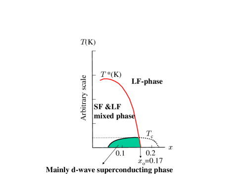
Figure 10: (Color online) New explanation for phase diagram of LSCO. Since $T^{*}(x)$, which is higher than $\tilde{T}^{*}(x)$, has not been calculated, its numerical values are not shown on the vertical axis.

Furthermore we can predict that the spin susceptibility will show 2D-like AF features mainly below $T^{*}(x)$ and Pauli-like temperature-dependent behavior above $T^{*}(x)$. We find that this prediction is also consistent with the experimental results for LSCO [49, 50]. In this context, it should be emphasized that the K-S model is shown to explain successfully not only the ARPES experimental results [10, 16, 47, 48] but also a number of other experimental results such as NMR results showing the coexistence of a superconducting state and AF order [32], polarized X-ray absorption spectra [56, 57], site-specific X-ray absorption spectroscopy [58], anomalous electronic entropy [59, 7], and d-wave superconductivity [60, 61]. Theoretically, the K-S model is also supported by LDA + U band calculations [33], as already mentioned in §2.5.

6 Conclusions and Concluding Remarks

In this study we have shown on the basis of the K-S model how the interplay of Mott physics and JT physics plays an important role in determining the superconducting state as well as the metallic state of underdoped cuprates. In connection with the interplay of JT physics and Mott physics, the following important results have been obtained in this study: It has been clarified on the basis of the K-S model that the concept of the pseudogap discussed theoretically[52, 62, 63] and reported by ARPES, STM, and tunneling experiments below $T^{*}(x)$ in underdoped cuprates [36, 37, 64] can be explained by the occurrence of Fermi pockets in the underdoped region without the pseudogap hypothesis. We have shown that the appearance of the broad hump observed in the antinodal region in ARPES can be explained by the real transitions of photoexcited electrons from the occupied states in the highest conduction band in the antinodal region to a free-electron state above the vacuum level. Furthermore, we have shown that the physical meaning of $T^{*}$ represents a crossover line from an inhomogeneous phase consisting of Fermi pockets and large FS in the normal state to a phase consisting of a large FS.

Finally, several remarks are made on the small FS and shadow bands in the underdoped regime of cuprates. In 1996, Wen and Lee developed a slave-boson theory for the t-J model at finite doping level, and showed that Fermi pockets at low doping continuously evolve into a large FS at high doping concentrations [65]. Although their theoretical model is different from the K-S model, it is interesting to find that they obtained a result similar to the result predicted using the K-S model in 1994 with regard to the change from a small FS to a large FS with increasing hole concentration. Recently, a proposal was made to reconcile the experimental result of the coexistence of antiferromagnetism and superconductivity [66]. Furthermore, in relation to the small FS, the idea of a shadow FS was proposed as a replica of the main FS transferred using $Q=(\pi/a,\pi/a)$ by Kampf and Schrieffer theoretically [67] and by Aebi et al. experimentally [68]. Investigating the validity of the idea of the shadow FS experimentally, the observation of shadow bands in ARPES spectra has been reported [69, 70, 71]. Responding to the problems of the shadow FS and shadow bands from the standpoint of the K-S model, it should be emphasized that Fermi pockets in the metallic state calculated from the K-S model have been derived as a result of the interplay of JT physics and Mott physics; thus, the origin of Fermi pockets is different from that in a single-component theory. Therefore, the Fermi pockets shown in Fig. 5 are neither the shadow FS nor related to the shadow bands.

- [1] P. W. Anderson: Science 235 (1987) 1196.
- [2] J. G. Bednorz and K. A. Müller: Z. Phys. B 64 (1986) 189.
- [3] N. Shima, K. Shiraishi, T. Nakayama, A. Oshiyama, and H. Kamimura: in Proc. 1st Int. Conf. Electronic Materials in New Materials and New Physical Phenomena for Electronics of the 21st Century, ed. T. Sugano, R. R. H. Chang, H. Kamimura, I. Hayashi, and T. Kamiya (Materials Research Society, Pittsburgh, 1989) p.51.
- [4] A. Oshiyama, N. Shima, T. Nakayama, K. Shiraishi and H. Kamimura: in Mechanism of High Temperature Superconductivity. Springer Series in Materials Science ed. H. Kamimura and A. Oshiyama (Springer, Berlin, Heidelberg, 1989) vol. 11, p.111.
- [5] H. Kamimura, H. Ushio, S. Matsuno and T. Hamada: Theory of Copper Oxide Superconductors (Springer, Berlin, Heidelberg, 2005)(Chap.4, p.31).
- [6] H. Kamimura and Y. Suwa: J. Phys. Soc. Jpn. 62 (1993) 3368.
- [7] H. Kamimura, T. Hamada and H. Ushio: Phys. Rev. B 66 (2002) 054504.
- [8] H. Kamimura and H. Ushio: Solid State Commun. 91 (1994) 97.
- [9] H. Ushio and H. Kamimura: J. Phys. Soc. Jpn. 64 (1995) 2585.
- [10] J. Meng, G. Liu, W. Zhang, L. Zhao, H. Liu, X. Jia, D. Mu, S. Liu, X. Dong, J. Zhang, W. Lu, G. Wang. Y. Zhou, Y. Zhu, X. Wang, Z. Xu, C. Chen, and X. J. Zhou: Nature 462 (2009) 335.
- [11] N. Doiron-Leyraud, C. Proust, D. LeBoeuf, J. Levallois, J.-B. Bonnemaison, R. Liang, D. A. Bonn, W. H. Hardy, and L. Taillefer: Nature 447 (2007) 565.
- [12] A. F. Bangura, J. D. Fletcher, A. Carrington, J. Levallois, M. Nardone, B. Vignolle, P. J. Heard, N. Doiron-Leyraud, D. LeBoeuf, L. Taillefer, S. Adachi, C. Proust, and N. E. Hussey: Phys. Rev. Lett. 100 (2008) 047004.
- [13] T. Yoshida, X. J. Zhou, M. Nakamura, S. A. Keller, P. V. Bogdanov, E. D. Lu, A. Lanzara, Z. Hussain, A. Ino, A. Fujimori, H. Eisaki, Z.-X Shen, T. Kakeshita and S. Uchida: Phys. Rev. Lett. 91 (2003) 027001.
- [14] T. Yoshida, X. J. Zhou, K. Tanaka, W. L. Yang, Z. Hussain, Z.-X. Shen, A. Fujimori, S. Sahrakorpi, M. Lindroos, R. S. Markiewicz, A. Bansi, S. Komiya, Y. Ando, H. Eisaki, T. Kakeshita, and S. Uchida: Phys. Rev. B 74 (2006) 224510.
- [15] S. Charkravarty and H.-Y. Kee: Proc. National Academy of Sciences of USA 105 (2008) 8835.
- [16] K. Tanaka, W. S. Lee, D. H. Lu, A. Fujimori, T. Fujii, Risdiana, I. Terasaki, D. J. Scalapino, T. P. Devereaux, Z. Hussain, and Z.-X. Shen: Science 314 (2006) 1910.
- [17] H. Kamimura and M. Eto: J. Phys. Soc. Jpn. 59 (1990) 3053.
- [18] M. Eto and H. Kamimura: J. Phys. Soc. Jpn. 60 (1991) 2311.
- [19] F. C. Zhang and T. M. Rice: Phys. Rev. B 37 (1988) 3759.
- [20] H. Kamimura, S. Matsuno, Y. Suwa, and H. Ushio: Phys. Rev. Lett 77 (1996) 723.
- [21] H. Kamimura, H. Hamada, S. Matsuno, and H. Ushio: J. Supercond. 15 (2002) 379.
- [22] See, for example, L. F. Mattheiss: Phys. Rev. Lett. 58 (1987) 1028.
- [23] See also J. Yu, A. J. Freeman and J.-H. Xu: Phys. Rev. Lett. 58 (1987) 1035.
- [24] J. M. Luttinger and J. C. Ward: Phys. Rev. 118 (1960) 1417.
- [25] T. Mason, A. Schroder, G. Aeppli, H. A. Mook and S. M. Haydon: Phys. Rev. Lett. 77 (1996) 1604.
- [26] K. Yamada, C. H. Lee, J. Wada, K. Kurahashi, H. Kimura, Y. Endoh, S. Hosoya, G. Shirane, R. J. Birgeneau and M. A. Kastner: J. Supercond. 10 (1997) 343.
- [27] K. Yamada, C. H. Lee, K. Kurahashi, J. Wada, S. Wakimoto, S. Ueki, H. Kimura, and Y. Endoh: Phys. Rev. B 57 (1998) 6165.
- [28] Y.-J. Kao, Q. Si, and K. Levin: Phys. Rev. B 61 (2000) R11898.
- [29] N. B. Christensen, D. F. McMorrow, H. M. Ronnow, B. Lake, S. M. Hayden, G. Aeppli, T. G. Perring, M. Mangkorntong, M. Nohara, and H. Takagi: Phys. Rev. Lett. 93 (2004) 147002.
- [30] J. M. Tranquada: Nature 429 (2004) 534.
- [31] S. M. Haydon, H. A. Mook, P. Dai, T. G. Perring and F. Dogan: Nature 429 (2004) 531.
- [32] H. Mukuda, M. Abe, Y. Araki, Y. Kitaoka, K. Tokiwa, T. Watanabe, A. Iyo, H. Kito, and Y. Tanaka: Phys. Rev. Lett. 96 (2006) 087001.
- [33] V. L. Anisimov, S. Yu Ezhov and T. H. Rice: Phys. Rev. B 55 (1997) 12829.
- [34] D. S. Marshall, D. S. Dessau, A. G. Loeser, C.-H. Park, A. Y. Matsuura, J. N. Eckstein, I. Bozovic, P. Fournier, A. Kapitulnik, W. E. Spicer, and Z.-X. Shen: Phys. Rev. Lett. (1996) 76.
- [35] M. R. Norman, H. Ding, M. Randeriat, J. C. Campuzano, T. Yokoya, T. Takeuchi, T. Takahashi, T. Mochiku, K. Kadowaki, P. Guptasarma, and D. G. Hinks: Nature 392 (1998) 157.
- [36] M. R. Norman, A. Kanigel, M. Randeria, U. Chatterjee, and J. C. Campuzano: Phys. Rev. B 76 (2007) 174501, and related references therein.
- [37] A. Kanigel, M. R. Norman, M. Randeria, U. Chatterjee, S. Souma, A. Kaminski, H. M. Fretwell, S. Rosenkranz, M. Shi, T. Sato, T. Takahashi, Z. Z. Li, H. Raffy, K. Kadowaki, D. Hinks, L. Ozyuzer and J. C. Campuzano: Nat. Phys. 2 (2006) 447.
- [38] Y. J. Uemura, L. P. Le, G. M. Luke, B. J. Sternlieb, W. D. Wu, J. H. Brewer, T. M. Riseman, C. L. Seaman, M. B. Maple, M. Ishikawa, D. G. Hinks, J. D. Jorgensen, G. Saito, and H. Yamochi: Phys. Rev. Lett. 66 (1991) 2665.
- [39] see T. Sato and T. Takahashi: in Comprehensive Semiconductor Science and Technology, ed. P. Bhattacharya, R. Fornari and H. Kamimura (Elsevier, Amsterdam, Oxford, 2011) Vol.1, Chap. 1.11.
- [40] A. Damascelli, Z. Hussain and Z.-X. Shen: Rev. Mod. Phys. 75 (2003) 473.
- [41] T. Mizokawa: private communication.
- [42] See, for example, G.-H. Gweon: Ph.D. Thesis, Dept. of Physics, University of Michigan, Michigan, (1999).
- [43] For the value of the work function for cuprates, see, for example, G. Kinoda, T. Hasegawa, S. Najao, T. Hamaguri, K. Kitazawa, K. Shimizu, J. Shimoyama, and K. Kishio: Phys. Rev. B 67 (2003) 224509.
- [44] H.-B. Yang, J. D. Rameau, P. D. Johnson, T. Valla, A. Tsvelik and G. D. Gu: Nature 456 (2008) 77.
- [45] T. Hamada, K. Ishida, H. Kamimura and Y. Suwa: J. Phys. Soc. Jpn. 70 (2001) 2033.
- [46] H. Kamimura and T. Hamada: in Models and Methods of High- Superconductivity: Some Frontal Aspects, ed. J. K. Srivastava and S. M. Rao (Nova Science Publisher, New York, 2003) Vol. 2, Chap. 2.
- [47] M. R. Norman, M. Randeria, H. Ding and J. C. Campuzano: Phys. Rev. B 57 (1998) R11093.
- [48] W. S. Lee, I. M. Vishik, K. Tanaka, D. H. Lu, T. Sasagawa, N. Nagaosa, T. P. Devereaux, Z. Hussain, and Z.-X. Shen: Nature 450 (2007) 81.
- [49] T. Nakano, M. Oda, C. Manabe, N. Momono, Y. Miura and M. Ido: Phys. Rev. B 49 (1994) 16000.
- [50] J. R. Cooper and J. W. Loram: J. Phys. I. France 6 (1996) 2237.
- [51] See, for example, N. Miyakawa, P. Guptasarma, J. F. Zasadzinski, D. G. Hinks, and K. E. Gray: Phys. Rev. Lett. 80 (1998) 157.
- [52] P. Wrobel, R. Eder and R. Micnas: J. Phys.: Condens. Matter 15 (2003) 2755.
- [53] P. Wrobel, R. Eder and P. Furde: J. Phys.: Condens. Matter 15 (2003) 6599.
- [54] K. A. Müller: Phil. Mag. Lett. 82 (2002) 279.
- [55] K. McElroy: Nat. Phys. 2 (2006) 441.
- [56] C. T. Chen, L. H. Jieng, J. Kuo, P. Rudolf, F. Sette and R. M. Fleming: Phys. Rev. Lett. 68 (1992) 2543.
- [57] E. Pellegrin, N. Nücker, J. Fink, S. L. Molodtsov, A. Gutierrez, E. Navas, O. Strebel, Z. Hu, M. Domke, G. Kaindl, S. Uchida, Y. Nakamura, J, Marki, M. Klauda, G. Saemann-Ischenko, A. Krol, J. L. Peng, Y. Li and R. L. Greene: Phys. Rev. B 47 (1993) 3354.
- [58] M. Merz, N. Nücker, P. Schweiss, S. Schuppler, C. T. Chen, V. Chakarian, J. Freeland, Y. U. Idzerda, M. Kläser, G. Müller-Vogt, and Th. Wolf: Phys. Rev. Lett 80 (1998) 5192.
- [59] J. W. Loram, K. A. Mirza, J.R. Cooper, and J. L. Tallon: J. Phys. Chem. Solids 59 (1998) 2091.
- [60] D. A. Wollman, D. J. Van Harlingen, J. Giapintzakis, and D. M. Ginsberg: Phys. Rev. Lett 74 (1995) 797.
- [61] C. C. Tsuei and J. R. Kirtley: Rev. Mod. Phys. 72 (2000) 969, and related references therein.
- [62] See J. Schmalian, D. Pines and B. Stojkovic: Phys. Rev. Lett. 80 (1998) 3839, and related references therein.
- [63] K.-Y. Yang, T. M. Rice and F.-C. Zhang: Phys. Rev. B 73 (2006) 174501, and related references therein.
- [64] Ch. Renner, B. Revaz, J.-Y. Genoud, K. Kadowaki, and O. Fischer: Phys. Rev. Lett. 80 (1998) 149.
- [65] X.-G. Wen and P. A. Lee: Phys. Rev. Lett. 76 (1996) 503.
- [66] R. K. Kaul, Y. B. Kim, S. Sachdev and T. Senthil: Nat. Phys. 4 (2008) 28.
- [67] A. Kampf and J. R. Schrieffer: Phys. Rev. B 41 (1990) 6399.
- [68] P. Aebi, J. Osterwalder, P. Schwaller, L. Schlapbach, M. Shimoda, T. Mochiku, and K. Kadowaki: Phys. Rev. Lett. 72 (1994) 2757.
- [69] Y. M. Vilk: Phys. Rev. B 55 (1997) 3870.
- [70] N. L. Saini, J. Avila, A. Bianconi, A. Lanzara, M. C. Asensio, S. Tajima, G. D. Gu and N. Koshizuka: Phys. Rev. Lett. 79 (1997) 3467.
- [71] K. Nakayama, T. Saito, T. Dobashi, K. Terashima, S. Souma, H. Matsui, T. Takahashi, J. C. Campuzano, K. Kubo, T. Sasaki, N. Kobayashi, T. Kondo, T. Takeuchi, K. Kadowaki, M. Kofu, and K. Hirota: Phys. Rev. B 74 (2006) 054505, and related references therein.