Negatively Biased Relevant Subsets Induced by the Most-Powerful One-Sided Upper Confidence Limits
for a Bounded Physical Parameter

Abstract

Suppose an observable $x$ is the measured value (negative or non-negative) of a “true mean” $\mu$ (physically non-negative) in an experiment with a Gaussian resolution function with known fixed rms deviation $\sigma$. The most powerful one-sided upper confidence limit at 95% confidence level (C.L.) is $\mu_{\rm UL}=x+1.64\sigma$, which I refer to as the “original diagonal line”. Perceived problems in HEP with small or non-physical upper limits for $x<0$ historically led, for example, to substitution of $\max(0,x)$ for $x$, and eventually to abandonment in the Particle Data Group’s Review of Particle Physics of this diagonal line relationship between $\mu_{\rm UL}$ and $x$. Recently Cowan, Cranmer, Gross, and Vitells (CCGV) have advocated a concept of “power constraint” that when applied to this problem yields variants of diagonal line, including $\mu_{\rm UL}=\max(-1,x)+1.64\sigma$. Thus it is timely to consider again what is problematic about the original diagonal line, and whether or not modifications cure these defects. In a 2002 Comment, statistician Leon Jay Gleser pointed to the literature on recognizable and relevant subsets. For upper limits given by the original diagonal line, the sample space for $x$ has recognizable relevant subsets in which the quoted 95% C.L. is known to be negatively biased (anti-conservative) by a finite amount for all values of $\mu$. This issue is at the heart of a dispute between Jerzy Neyman and Sir Ronald Fisher over fifty years ago, the crux of which is the relevance of pre-data coverage probabilities when making post-data inferences. The literature describes illuminating connections to Bayesian statistics as well. Methods such as that advocated by CCGV have 100% unconditional coverage for certain values of $\mu$ and hence formally evade the traditional criteria for negatively biased relevant subsets; I argue that concerns remain. Comparison with frequentist intervals advocated by Feldman and Cousins also sheds light on the issues.

1 Introduction

In high energy physics (HEP), a prototype problem with far-reaching implications and generalizations is that in which an observable $x$ is the measured value (negative or non-negative) of a “true mean” $\mu$ (physically non-negative) in an experiment with a Gaussian resolution function with fixed rms deviation $\sigma$, assumed known for most of this discussion. Typically the scientific context has been searches to establish a non-zero value of $\mu$ that would signal a discovery (non-zero neutrino mass; existence of a rare process; etc.). In the absence of a signal, traditionally one would set an upper limit $\mu_{\rm UL}$ on $\mu$ at specified confidence level (C.L.),

$$\mu_{\rm UL}=x+1.64\sigma\ {\rm(95\%C.L.),}$$ (1)

or $\mu_{\rm UL}=x+1.28\sigma$ (90% C.L.). I refer to this method as the “original diagonal line”, defined by one-tailed integrals with 5% and 10% tail probabilities, respectively.

Figure 1 displays Eqn. 1 in the form of a confidence belt. (In the figure and much of this paper, $\sigma$ is set to 1 without loss of generality. Equivalently, $\mu$ and $x$ are to be interpreted as $\mu/\sigma$ and $x/\sigma$, respectively.) For each possible value of the unknown true value of $\mu$ (vertical axis), there is a horizontal line (“acceptance interval”, drawn for representative values of $\mu$) such that there is a 95% probability that the observed $x$ is within that line. Upon observing a value of $x$, one draws a vertical line through the observed value. The quoted confidence interval for $\mu$ consists of those values of $\mu$ for which the associated horizontal line is intersected by the vertical line, in this case thus recovering Eqn. 1. For $x<-1.64$, the confidence interval is thus the empty set. Nonetheless, this confidence belt has the property that no matter what the true value of $\mu$ is, 95% of the quoted confidence intervals will contain (“cover”) that value. Furthermore, this belt gives the tightest limits (corresponding to a “most powerful” test) of all one-sided belts.

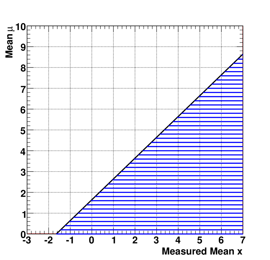
Figure 1: Confidence belt corresponding to the original diagonal line at 95% C.L., as described in the text. Negative values of $\mu$ do not exist in the model, so for $x<-1.64$, the set of values of $\mu$ not excluded is the empty set. Here and in other figures, $\sigma=1$ without loss of generality. (Equivalently, $\mu$ and $x$ are $\mu/\sigma$ and $x/\sigma$, respectively.)

Historically, as $x$ became small, negative, or very negative, increasing levels of discomfort would set in among many physicists. When the formal results from using Eqn. 1 yielded $\mu_{\rm UL}<0$, some described the upper limit as “unphysical” rather than the empty set, but in any case the experimenter was faced with a problem. In a 1986 note [1], Virgil Highland summarized six recipes (here converted to 95% C.L. if used), three based on the diagonal line of Eqn. 1.

One possibility, referred to by Highland as the “Truncated Classical Method”, was to replace the negative or empty-set upper limit of Eqn. 1 (obtained when $x<-1.64$) with $\mu_{\rm UL}=0$. That is, $\mu_{\rm UL}=\max(0,x+1.64)$, with the corresponding confidence belt shown in Fig. 2. I do not know if $\mu_{\rm UL}=0$ was ever used in a publication. In the 2008–2009 Higgs statistical combination study in Ref. [2], ATLAS describes a method which again yields $\mu_{\rm UL}=\max(0,x+1.64)$. This method is used by the 2011 ATLAS supersymmetry searches published in Refs. [3, 4], apparently without encountering the case $\mu_{\rm UL}=0$. (A “power constrained” modification also used by ATLAS is described below.)

Figure 2: Modification of the confidence belt in Fig. 1 by replacing the empty-set interval for $x<-1.64$ with the single point $\mu_{\rm UL}=0$. The acceptance interval for $\mu=0$ thus contains 100% of the probability for $x$ values rather than 95%. In 1986, Highland [1] referred to this as the “Truncated Classical Method”. The same result comes from the derivation in the 2008–2009 ATLAS studies [2].

A more common notion was to use $\max(0,x)$ rather than $x$ in Eqn. 1, i.e., to move the measured value $x$ to the physical boundary and proceed, obtaining $\mu_{\rm UL}=1.64$. The corresponding belt (Fig. 3) has 100% coverage for $\mu\leq 1.64$.

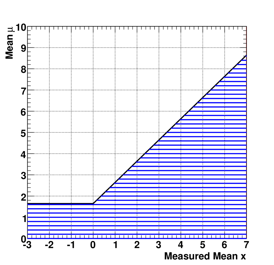
Figure 3: Modification of the confidence belt in Fig. 1 by using the $\mu_{\rm UL}$ for $x=0$ when $x<0$, so that $\mu_{\rm UL}=\max(0,x)+1.64$. The same result is obtained by using a Power Constrained Limit of CCGV [5] with 50% power constraint.

There was however a sense among many (correct in my view) that the problem with these diagonal line solutions with horizontal-line modifications was fundamental and could not be patched up merely by imposing a minimum value of $\mu_{\rm UL}$ or of $x$. There was much discussion in the 1980’s and 1990’s, leading to the 2000 Confidence Limits Workshops [6, 7] which evolved into the PhyStat conference series. During this period, three methods gained significant support in HEP for constructing intervals that departed from those based on the diagonal line: a Bayesian method (called “very usual” by Highland [1] in 1986) with some basis in the statistics literature; a method invented at LEP called CL_S [6] that used reasoning apparently not in the statistics literature and took advantage of some numerical coincidences; and a method advocated by Feldman and Cousins (F-C) [8], which we learned was in Kendall and Stuart [9]. The Particle Data Group’s Review of Particle Physics (PDG RPP) [10] abandoned the diagonal line and described these three methods beginning, respectively, in 1986, 2002, and 1998. For this simple problem, the Bayesian and CL_S belts are the same, shown in Fig. 4.

Figure 4: Upper limits obtained via the Bayesian method recommended by the PDG RPP, plotted as a confidence belt. The prior probability density for $\mu$ is uniform for all $\mu$ which exist in the model, i.e., for $\mu\geq 0$. The horizontal lines contain more than 95% of the acceptance for $x$, so from the frequentist point of view the upper limits are conservative. For this problem, the upper limits from CL_S are the same.

The F-C belt, displayed in Fig. 5, has a non-zero lower edge for $x>1.64$, as discussed below.

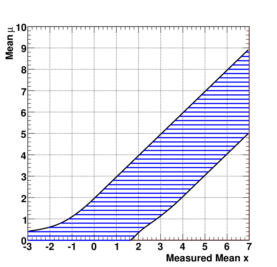
Figure 5: 95% confidence belt advocated by Feldman and Cousins [8]. For $x\leq 1.64$, the lower end of the interval is 0. All horizontal acceptance intervals contain 95% of the probability for observing $x$.

As an alternate protection against limits deemed to be “anomalously strong” (such as those obtainable from Fig. 2), a concept of “Power Constrained Limit” was advocated by Cowan, Cranmer, Gross, and Vitells (CCGV) [5], and applied to ATLAS Higgs searches [11, 12], including the July 2011 submission in Ref. [13]. The method, as described in some detail in Ref. [12] and used in Ref. [13], follows the recommendation of CCGV [5] (also cited by another ATLAS supersymmetry search [14]), which for the example at hand yields $\mu_{\rm UL}=\max(-1,x)+1.64$. (This corresponds to a power constraint [5] of 16%.) The corresponding belt is shown in Fig. 6. The old belt of Fig. 3 turns out to correspond to a Power Constrained Limit with a power constraint of 50%, which was considered “too extreme” at the time Ref. [5] was posted (16 May 2011). Since then, PCL proponents and ATLAS have reconsidered, and a more recent Higgs combination note [15] uses a 50% power constraint.

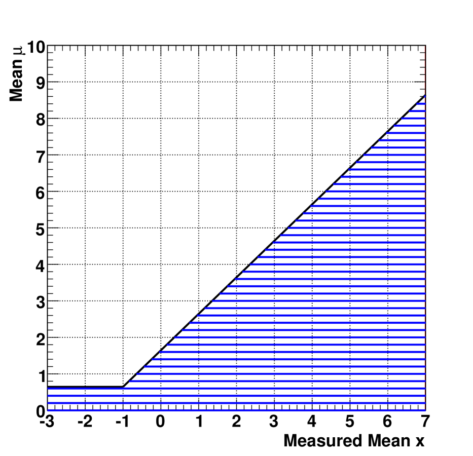
Figure 6: Upper limits obtained by the “Power Constrained Limit” method following the recommended 16% power constraint of CCGV [5] which leads to $\mu_{\rm UL}=\max(-1,x)+1.64$.

Thus it is timely to consider again what is problematic about the original diagonal line of Eqn. 1, and whether or not modifications such as replacing $x$ with $\max(0,x)$ or $\max(-1,x)$ get to the root of these problems.

My views in 1998-2000, still largely unchanged, are discussed in the Refs. [6] and [8]. An issue that we called “flip-flopping” and its resolution is discussed in detail in Ref. [8]. Another point in Ref. [8], explained in more detail below in Sec. 2.1, is how the diagonal line of Fig. 1 undesirably couples together goodness of fit for the model with interval estimation of parameters of the model. However, in most of this paper I focus on following the additional leads given by statisticians in commenting on a 2002 review paper by physicist Mark Mandelkern [16]. In particular, the statistician Leon Jay Gleser [17] pointed to the literature on recognizable and relevant subsets which gives great insight into the problem from a different (though of course related) perspective than we have had before.

The discussion points to quite remarkable theorems and examples in the statistics literature. The concept of “most powerful hypothesis test” in the sense of Neyman and Pearson (N-P) can be in direct conflict with a scientist’s desire to extract the most relevant inference from a particular data set at hand. Desiderata have been formulated in terms of pure conditional frequentist probabilities that lead to a connection to Bayesian statistics, even though the conditional frequentist probabilities discussed in this context have the usual interpretation with the endpoints of the intervals as the random variables. The connection (still not completely known) has to do with whether there exists any (possibly generalized) Bayesian prior that leads to Bayesian credible intervals similar to the confidence intervals in the frequentist confidence set; this can have some relation to whether or not the sample space for $x$ has recognizable subsets for which the experimenter knows that the frequentist coverage is different from nominal in that subset.

If one’s data is in such a recognizable subset, what to do is likely context dependent. But for searches for New Physics, I would side with those who argue to make the frequentist-based inference as relevant as it can be within the constraints of coverage. (Ref. [8] still is my preferred way to do this.) I have also advocated for some time performing as well a Bayesian analysis, which uses only the “relevant” probability of obtaining the data at hand, but for which repeated sampling properties or prior sensitivity may be unsatisfactory. By comparing the two, one gets even greater insight into any problem.

Section 2 introduces Fisher’s concept of recognizable subsets of the sample space, using the example of the much-discussed issue of empty intervals. A reminder of the issue of coupling goodness of fit and interval estimation is included at the end of this section. Section 3 describes the half-century-old formalism and definitions for studying conditional coverage within subsets, and some subsequent results and concepts from the statistics literature. Section 4 applies these concepts to the original diagonal line of Eqn. 1, thus revealing the troublesome property, negatively biased relevant subsets, in the language introduced in Sec. 3. Section 5 discusses methods which add a horizontal line to the original diagonal line. Methods such as these, having 100% unconditional coverage for some values of $\mu$ while stating “95% C.L.”, are not considered in the literature I have seen on relevant subsets; I believe that a careful adaptation would raise some analogous concerns. I conclude in Sec. 8, along with comparisons to the intervals advocated by F-C in Ref. [8].

2 A simple betting game

Suppose that Peter performs a set of repeated experiments, and after each experiment, he uses the observed $x$ and Eqn. 1 to announce, “Using a procedure which is guaranteed to cover the unknown true value of $\mu$ in 95% of experiments, and fail to cover in 5% of experiments, I assert that the true value of $\mu$ is less than or equal to $x+1.64$.” Suppose then that Paula says, “OK, in that case, you should be willing to offer to bet against me at 19:1 odds that each of your assertions is true. Let us play the following game. After each experiment, I will decide, based on the value of $x$ you obtain, whether or not to bet against the assertion you made following that experiment, and I will do this using no more information about the model or $\mu$ than you have (in particular without using any prior knowledge of the true $\mu$).” Peter says fine.

Paula then proceeds to bet against Peter’s assertion whenever $x<-1.64$, and to say “no thanks” to the bet whenever $x\geq-1.64$. Paula not only wins in the long run – in fact she wins every bet! As described in Sec. 4, Paula can in fact win in the long run by accepting all bets (at 19:1 odds) if $x<C$, where $C$ is any constant of her choice. E.g., for $C=0$, she wins at least 10% of the bets, well above her break-even point of 5%.

Since Paula is winning bets by using no more information than that available to Peter, it is certainly arguable that Peter is not making the most relevant assertions about each of his data sets. This example has much in common with a number of disturbing examples in the statistics literature in which the N-P theory of tests that are most powerful in the long run can lead to statements that appear to be irrelevant or misleading for interpreting a particular data set at hand. The “modern” discussion seems to have been stimulated by Sir Ronald Fisher (reprinted in [18]) who coined the phrase “recognizable subset” in 1956 to describe a subset of “entities” for which it can be recognized that the probabilities associated with entities in the subset are different from their (still purely frequentist) probabilities in the superset of which the subset is a part.

Classic examples include Sir David Cox’s 1958 mixture experiment [19] with two measuring devices with different $\sigma$, one device chosen randomly as part of the repeated experimental procedure. Another classic example is interval estimation for the mean $\mu$ of a distribution uniform over $[\mu-1/2,\mu+1/2]$, based on a data set consisting of two sampled values $x_{1}$ and $x_{2}$. N-P procedures based on power give the same confidence interval (or confidence limit) for the data $\{x_{1}=0.99,x_{2}=1.01\}$ as for data $\{x_{1}=.51,x_{2}=1.49\}$, even though the second set restricts $\mu$ to the narrow range [0.99,1.01], while the first set only restricts $\mu$ to [0.51,1.49]. These two examples are particularly clean because in each there exists an ancillary statistic, conceptually a function of the data carrying information about the precision of the measurement but no information about $\mu$. (The ancillary statistic is the index of the detector used in the Cox example, and $|x_{2}-x_{1}|$ in the second example.) The ancillary statistics can be used to divide the sample space into subspaces for calculating conditional coverage probabilities relevant to the data at hand.

In these examples, there is a clear conflict between the criterion of maximum power in N-P tests and the notion (however vague at this point) of “using all of the available relevant information in the data set at hand”. This conflict was pursued in a landmark 1959 paper by Robert Buehler [20] (brought to our attention by Gleser [17]), in which he introduced a betting game such as that above and defined the terminology as described in the following section (which modernizes his Paul to Paula, but otherwise mostly transcribes part of Buehler’s paper). A key observation is that even in the absence of ancillary statistics, one can sometimes place bounds (away from the nominal C.L.!) on coverage probabilities within recognizable subsets of the sample space.

2.1 Coupling of goodness of fit and interval estimation

Another, less complete, view [8] of a difficulty of the original diagonal line is that it couples together goodness of fit (test of the model as a whole) with interval estimation (finding preferred values of the parameters assuming that the model is true). These two concepts are best kept separate, as is normally done in curve-fitting when one uses the magnitude of $\chi^{2}$ at the best-fit parameters as (only) a test of goodness of fit of the model, while using $\Delta\chi^{2}$ with respect to the minimum value to obtain an approximate confidence region for the parameters [10]. For the Gaussian problem at hand of restricting $\mu$ based on measured $x$, we have

$$\chi^{2}(\mu)=(x-\mu)^{2};\ \mu\geq 0.$$ (2)

Let us consider the case where the measurement obtains $x=-1$. The minimum $\chi^{2}$ is on the boundary, at $\mu=0$: $\chi^{2}_{\rm min}=\chi^{2}(\mu=0)=1.$ The upper limit from the diagonal line of Eqn. 1 is $\mu_{\rm UL}=-1+1.64=0.64$. We note that $\chi^{2}(\mu=0.64)=(-1-0.64)^{2}=2.70$. Thus, the 95% upper limit allows $\mu$ for which absolute $\chi^{2}\leq 2.70$. But 2.70 is the usual “book value” [10] of the difference $\Delta\chi^{2}$ to be used in computing a one-tailed upper limit! The fact that $\chi^{2}$ for $x=-1$ cannot be less than 1 for physical $\mu$ is somehow not used in computing the upper limit, as values with $\Delta\chi^{2}>2.70-1=1.70$ are excluded. This feature remains with the Power Constrained Limit if the recommendation of CCGV [5] is followed (even though Ref. [5] uses $\Delta\chi^{2}$), as a consequence of forcing the limit to be one-sided.

In the same way, for $x<-1.64$, the entire model is rejected by a goodness of fit test at 95% C.L. But if one accepts the model and asks what values of the parameters are preferred given that the model is true, it would seem somewhat useless to report the empty set.

To repair the situation from this point of view, the F-C paper [8] advocates intervals based on $\Delta\chi^{2}$ considering values of $x$ on both sides of $\mu$ in the construction of the acceptance intervals; for specified C.L., the critical value of $\Delta\chi^{2}$ is associated with each $\mu$, not with $x$. The result is the belt in Fig. 5.

3 Buehler’s betting game and subsequent literature

Following Buehler [20], we let $A$ denote Peter’s assertion about $\mu$ being in a particular interval, and let $P(A)$ denote the (frequentist) probability that $A$ is true in the unconditional sample space (all possible values of $x$). If Peter’s intervals are confidence intervals obtained from a Neyman construction with C.L. $\gamma$, then $P(A)=\gamma$, independent of $\mu$. Using knowledge of Peter’s rule $R$ for constructing confidence intervals, Paula adopts a strategy that consists of specifying in the unconditional sample space (also called observation space) two subsets $C^{+}$ and $C^{-}$ such that:

• For observations in $C^{+}$, Paula bets that $A$ is true, risking $\gamma$ to win $1-\gamma$.

• For observations in $C^{-}$, Paula bets that $A$ is false, risking $1-\gamma$ to win $\gamma$.

It is not required that a bet must always be made; i.e., the union of $C^{+}$ and $C^{-}$ need not be the unconditional space. To determine the winner of each bet, we postulate the existence of a referee who knows the true value of $\mu$.

We thus focus on the conditional probabilities $P(A|C)$. Buehler calls $P(A|C)-\gamma$ the bias of $C$. Then in typical interval estimation problems, the bias of most subsets $C$ will not have the same sign for all $\mu$. Paula’s task is to find subsets $C$ whose bias has the same sign for all $\mu$. These are called semi-relevant subsets induced by the rule $R$. If in addition the bias is bounded away from zero, they are called relevant, a stricter requirement than semi-relevant. That is:

1. $C$ is a semi-relevant subset induced by the rule $R$ if either:

   1. $P(A|C)>\gamma$ for all $\mu$, or

   2. $P(A|C)<\gamma$ for all $\mu$;

2. $C$ is a relevant subset induced by the rule $R$ if, for some constant $c>0$ independent of $\mu$, either

   1. $P(A|C)\geq\gamma+c$ for all $\mu$, or

   2. $P(A|C)\leq\gamma-c$ for all $\mu$;

where “$>$” or “$\geq$” indicates positive bias (overcoverage), and “$<$” or “$\leq$” indicates negative bias (undercoverage).

Thus, for a negatively biased semi-relevant subset, there is conditional undercoverage for all $\mu$, but there exist $\mu$ for which the conditional undercoverage is arbitrarily small. For a negatively biased relevant subset, the conditional undercoverage is bounded away from $\gamma$ by at least a finite amount $c$ for all $\mu$.

All of these probabilities $P$ are frequentist probabilities: assertions about confidence intervals/regions and limits are assertions to be evaluated in terms of frequentist coverage in the usual sense. That is, the endpoints of the interval (or boundary of the confidence regions in higher dimensions) are the random variables, not $\mu$, which is unknown and for which $P(\mu)$ need not be defined. The issue is about which ensemble to use for calculating coverage properties for post-data inference, either the whole sample space (as Neyman advocated), or some “recognizable” sub-space $C$ in which the obtained data lies (as Fisher advocated).

One might hope that in a typical interval estimation problem, there are no relevant or semi-relevant subsets, i.e., for any $C$, there exists some $\mu$ for which $P(A|C)=\gamma$. Buehler calls this strong exactness; he refers to the usual unconditional coverage $P(A)=\gamma$ as weak exactness. But Buehler and subsequent authors found semi-relevant subsets to be quite common in frequentist confidence sets, so that “nonexistence of semirelevant subsets is a very severe requirement indeed.” Relevant subsets have also been identified in some famous problems, forcing one to think hard about post-data inference in these cases. A number of theorems were proven giving necessary or sufficient conditions for the existence of relevant or semi-relevant subsets. Very significantly, a deep relation with Bayesian theory was already noted by Buehler and by David L. Wallace [21] in the same year. The “very severe requirement indeed” of strong exactness was proven [21] to be automatically satisfied if there exists any (proper) Bayesian prior such that each interval in the set of frequentist confidence intervals also has Bayesian posterior probability $\gamma$, i.e., each interval also has Bayesian credibility $\gamma$.

The thread continued through key papers by Donald A. Pierce [22], James V. Bondar [23], G.K. Robinson [24], and very helpful reviews by George Casella [25] and by Constantinos Goutis and George Casella [26]. Buehler’s betting framework was generalized, for example by letting Paula adjust the odds to make more precise use of her conditional coverage calculation. Pierce and Robinson furthered the connections to Bayesian statistics, generalizing the results showing that Bayesian procedures with proper priors induce no semirelevant functions, and proving some more limited statements about the converse. (A succinct summary is in Ref. [25].) Connections were made to decision theory as well.

Bondar referred to the absence of relevant or semi-relevant sets as “consistency principles”. By the time of his paper, there were enough examples of otherwise-reasonable confidence sets admitting semi-relevant subsets (of both signs of bias) and relevant subsets of positive bias (i.e., overcoverage), that Robinson, Bondar, and others seemed to reach a consensus that the criterion of “elimination of negatively biased relevant subsets was about right” [25]. This is about as much as one can demand within the frequentist framework: to go further, one must use Bayesian credible intervals and in some problems lose the guarantee of weak exactness (unconditional coverage). The complete connection between conditional coverage and Bayesian procedures is still not known (in particular for improper priors).

4 Relevant subsets induced by the original diagonal line

Remarkably, to my knowledge Gleser’s Comment [17] is the first connection made in the statistics literature between all of this relevant-subset theory and our HEP problem of a physically bounded parameter:

The subset of samples having the property that the sample mean is two standard deviations to the left of zero would have been called a ‘recognizable subset’ by Fisher (1956)…Professor Mandelkern’s example shows that the classic Neyman confidence interval is not conditionally admissible in the case of estimating a positive mean. Extension of this result to other cases of bounded parameters is obvious. In short, once something about the data is known, it is possible for the frequentist properties of the confidence interval to change: the pre-data measure of risk is not necessarily the correct post-data measure of uncertainty. ([17], italics in original.)

Indeed it is not hard to work out the negative bias in relevant subsets induced by the original diagonal line of Eqn. 1. For example, Paula can define a relevant subset $C$ in the sample space by $x\,:\,x<0.7$. So she bets against Peter’s assertion $A$ at 19:1 odds whenever $x<0.7$. To see how she fares, we need to calculate, for each $\mu$, the conditional coverage probability $P(\mu\leq\mu_{\rm UL}\,|\,x<0.7)=P(x\geq\mu-1.64\,|\,x<0.7)$. This probability is maximum for $\mu=0$, in which case it is $P(x\geq-1.64\,|\,x<0.7)$, for $x$ sampled from a Gaussian centered at 0. That is easily computed from two tails to be $1-(0.05/0.758)=93.4\%$, negatively biased towards undercoverage. Paula concludes that the true conditional odds in Peter’s favor are at most 0.934/0.066, about 14:1, so she will win in the long run if Peter pays out at 19:1 odds on the bets she makes.

Figure 7 displays the conditional coverage $P(A|C)$, for that $\mu$ having the highest $P(A|C)$, where the relevant subset $C$ is in the form of this example, defined by $x<x_{\rm crit}$, with the value of $x_{\rm crit}$ on the horizontal axis. As in the simple betting example in Sec. 2, for $x_{\rm crit}<-1.64$, 0% of Peter’s assertions are true. At $x_{\rm crit}=0$, the conditional coverage increases to 90% (with Type I error probability of 10%, twice the nominal 5%). For larger $x_{\rm crit}$, $P(A|C)$ further increases, asymptotically approaching the unconditional 95% as $x_{\rm crit}$ rises above 1, and the effect of the boundary is less and less.

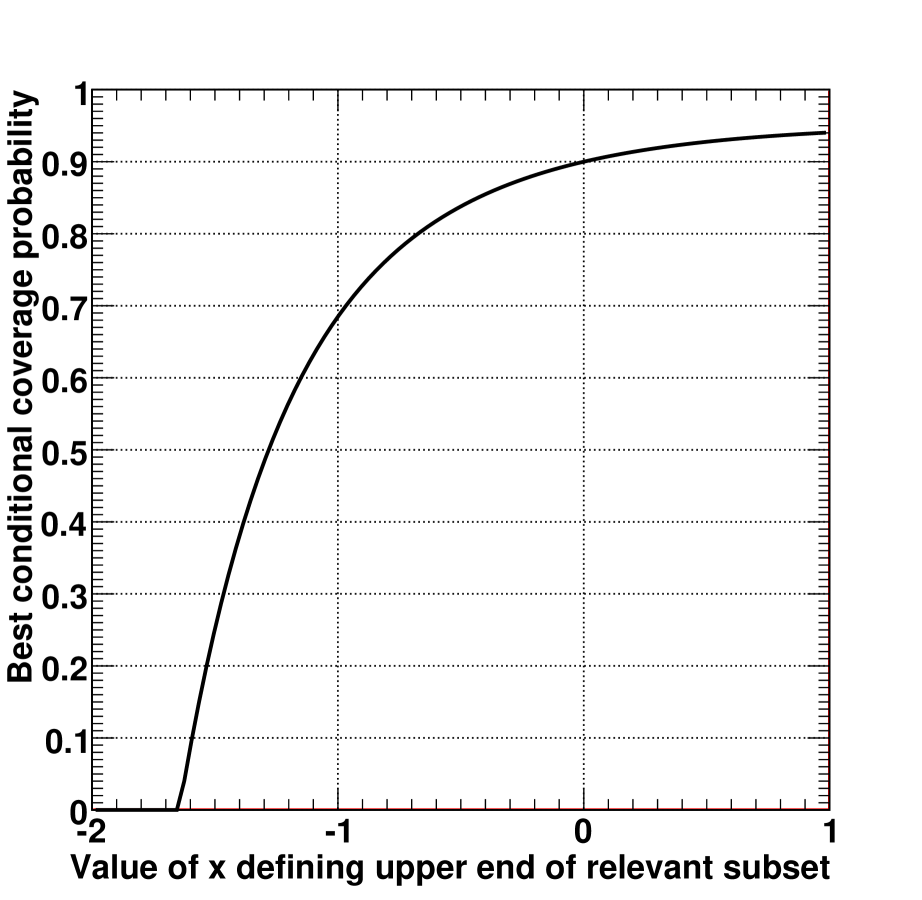
Figure 7: Best conditional coverage $P(A|C)$ (for that $\mu$ having the highest $P(A|C)$) vs. $x_{\rm crit}$, where Paula defines the recognizable subset $C$ by $x<x_{\rm crit}$. The recognizable subsets are negatively biased relevant subsets since the conditional coverage is less than of 0.95 by a finite amount.

Figure 7 thus quantifies for this problem the issue of using only pre-data measures of uncertainty based on unconditional probabilities (coverage, power) to distinguish among choices of hypothesis tests. I believe that it confirms physicists’ intuition of the past decades that the original diagonal line creates severe problems for making relevant interpretations about $\mu$ from the data set at hand. What is perhaps new is that we can see readily that these problems persist even beyond the “obvious” concerns that one had when $x$ was less than $-1.64$ (empty-set or unphysical upper limit), or when $x$ was only slightly larger than $-1.64$ (unnaturally small upper limit with $\mu_{\rm UL}\ll\sigma$).

5 Confidence belts with 100% acceptance intervals for some values of $\mu$

The above theory of relevant subsets is based on the situation in which the unconditional coverage of all values of $\mu$ is that stated by the confidence level $\gamma$, 95%. This is the case for the original diagonal line (Fig. 1) and for the F-C intervals (Fig. 5). As frequentist measures do not average conditional coverage over $\mu$, the definitions are all based on suprema of conditional coverage. If there is any single value of $\mu$ for which the horizontal acceptance interval for $x$ is the entire horizontal line $(-\infty,+\infty)$, then the coverage of the set of confidence intervals is 100% for that value of $\mu$. This is the case, for example, with Fig. 2, which has 100% coverage for $\mu=0$. Thus all conditional coverage calculations for $\mu=0$ also yield 100%, and thus the supremum of conditional coverage over all $\mu$ is also 100%. The formal theory of relevant subsets is thus rendered moot by adding a single value of $\mu$ with acceptance interval $(-\infty,+\infty)$ ! (A 100% acceptance interval for $\mu=3.14159$ would do so as well.) Paula cannot be sure of winning bets from Peter in the long run, because she will lose if the true $\mu$ is zero.

Should this evasion of the theory of relevant subsets, by having acceptance intervals with 100% acceptance, make physicists feel better about the upper limits in Fig. 2? I am not inclined to set aside the insights of Sec. 4 simply because the formal theory based on suprema is rendered moot. The same is true for methods which include yet more values of $\mu$ in the set with 100% coverage. This fact remains: If the true value of $\mu$ is one for which the unconditional coverage is equal to the stated confidence level of 95%, then there exist sets $C$ for which the conditional coverage of that $\mu$ is still bounded away from 95%. Thus, the supremum of conditional coverage over those values of $\mu$ for which the unconditional coverage is 95% is also bounded away from 95%.

If we consider, for example, the Power Constrained Limit of Fig. 6 with $\mu_{\rm UL}=\max(-1,x)+1.64$, Ref. [5] points out that the coverage is 100% for $\mu\leq 0.64$, while remaining exactly $\gamma=95$% for $\mu>0.64$. We can thus consider the conditional coverage properties for the entire set of $\mu$ for which the unconditional coverage is 95%. I.e., in the definitions in Sec. 3, we interpret “for all $\mu$” to mean “for all $\mu$ for which the unconditional coverage is $\gamma$”. For any set $C$, we find the maximum conditional coverage among the $\mu$ for which the unconditional coverage is $\gamma$. We observe that the conditional coverage of $\mu=0.65$ for $x_{\rm crit}=-1$ is 0, and the conditional coverage of $\mu=0.65$ for $x_{\rm crit}=0.65$ is 90%. That is, one shifts the curve in Fig. 7 horizontally by 0.64 to obtain the upper bound on the conditional coverage among those $\mu$ for which the unconditional coverage is stated (correctly) to be 95%.

Is this a useful assessment of the conditional properties of Power Constrained Limits? Perhaps not, but I do not know a better way to generalize the assessment of conditional properties of “95% C.L. upper limits” in the presence of acceptance intervals which have 100% acceptance. It seems to me that the burden should be on those advocating PCL to explain how the theory of relevant subsets can be adapted to this situation, so that it is possible to provide a more useful critique.

6 The frequentist alternative advocated by F-C

In the problem at hand, if one is willing to revisit the insistence on one-sided limits, then there is a better performing alternative rule $R$ for constructing confidence intervals, namely that advocated by Gary Feldman and myself [8]. This “unified approach” uses a likelihood-ratio (LR) ordering principle, i.e., inverting the likelihood-ratio test described in Kendall and Stuart [9]. We set out to eliminate the empty-set intervals in the much-discussed “Simple Betting” problem described in Sec. 2 in the context of searches for neutrino oscillations, and discovered along the way that the problem was deeply related to the insistence on having a one-sided limit, an insistence that we believed was grounded more in convention rather than any deep physics requirement.

If one wants to avoid empty-set intervals, then the logic leading from exact coverage to the necessity of two-sided intervals (the “unified approach” [8] in which the lower endpoint of the confidence interval is zero for only part of the sample space) is quite straightforward. In the Neyman construction, the acceptance region for $\mu=0$ must include all $x\leq 0$ in order to guarantee no empty-set intervals. In order for the acceptance region for $\mu=0$ to contain exactly $\gamma=95$% of the sample space probability, the upper endpoint must therefore be $x=1.64$. Hence for $x>1.64$, the confidence interval does not contain $\mu=0$. This simple argument is true as well for any other ordering rule (such as that preferred by Mandelkern yielding a different set of unified intervals [16]) which has exact coverage $\gamma$ for all values of $\mu$ and no empty-set intervals.

Incidentally, this “one-tailed” calculation of the upper endpoint of the F-C acceptance region for $\mu=0$ also explains clearly why the “unified approach” delivers exactly what high energy physicists are used to using in quantifying a discovery claim. The classical hypothesis test for rejecting $\mu=0$ at 5$\sigma$ is dual to constructing confidence intervals at C.L. $\gamma=1-2.8\times 10^{-7}$ and checking if $\mu=0$ is in the confidence interval. The F-C interval at this C.L. contains $\mu=0$ if and only if $x\leq 5\sigma$, as desired.

The unconditional coverage of the LR-ordering rule advocated by F-C is exact by construction. Since it is a frequentist rule which violates the likelihood principle, perhaps there are semi-relevant subsets induced by it, but I have not found them. I would expect any conditional bias induced by the LR-ordering to be vastly ameliorated compared to that of the original diagonal line.

7 Should the inference about $\mu$ be independent of $x$ for $x<0$?

Gleser’s Comment [17] on Mandelkern’s review [16] made another deep point not yet mentioned in the present paper. If the model assumes that $\sigma$ is known exactly, then the Likelihood Principle implies that one should make more restrictive inferences about $\mu$ as $x$ becomes more negative; this is the case for Bayesian upper limits (Fig. 4) and F-C intervals (Fig. 5), but not the case for the old method of using $\max(0,x)$ (Fig. 3) or for the Power Constrained Limit of Fig. 6 (or for the version of the unified approach advocated by Mandelkern). Gleser notes,

…any confidence intervals that keep a constant width as $X$ becomes more negative, as some of the physicists seem to desire, are indicating not necessarily what the data shows through the model and likelihood, but rather desiderata imposed external to the statistical model.

As suggested by several Comments on Mandelkern’s paper, if one is unhappy with inferences becoming too restrictive, one should expand the model to include uncertainty on $\sigma$.

8 Discussion and conclusion

In retrospect, I believe that the HEP community that abandoned the diagonal line of Eqn. 1 (for most of the issues of the PDG RPP [10] since 1987) understood a lot intuitively and from studying many examples before and since. With Gleser having pointed us to “relevant” literature, we can now make the conditional frequentist arguments which further illuminate the issues with original diagonal line of Eqn. 1. The increased power that one got from using the original diagonal line rather than the methods in the PDG RPP seemed to incorporate inappropriate information (for example goodness of fit to the model) that was hard to quantify. Now we can see that while the rule $R$ of the original diagonal line has perfect coverage and maximal power against one-sided alternatives, it induces severely negatively biased relevant subsets: one is making assertions that under-cover (for all values of $\mu$) for data in the recognizable relevant subset in which one’s obtained measurement lies.

With a better understanding of the issue of conditional coverage, we can also better understand why the Neyman-Pearson concept of pre-data unconditional probabilities should not be trusted to address all these difficulties. Of course power is a tremendously useful concept which we use in most contexts without conflict with other desiderata. But once the problem with the upper limits was identified as a conflict between pre-data and post-data assessment of confidence, the illuminating points naturally came from outside the Neyman-Pearson paradigm, using ideas built on those of Neyman’s great 20th century frequentist rival, Sir Ronald Fisher. Since the mathematics exposing the bias induced by the original diagonal line is based on the situation in which “95%” really means “95%”, modifications to include acceptance intervals of 100% would seem to require more generalized assessment tools. I believe that the problem cannot be easily dismissed in the absence of such tools: it is hard for me to imagine that the underlying diseases of Fig. 1 are eliminated simply by changing to Fig. 2 with the addition of a horizontal line at $\mu=0$. As this is the step which renders moot the relevant-subset literature, it is also not at all clear that subsequently imposing a further step of “power constraint” addresses this issue.

In the past, there had also been the rather vague notion that if there was no Bayesian calculation (with any prior) that gave credible intervals with some similarity to the confidence intervals, then the frequentist calculation could be “in trouble” of some sort. But it was hard to quantify such “violations of the Likelihood Principle”, and these ideas were not always convincing to those claiming to be “pure frequentist”. Thus it is extremely enlightening to see the theorems which relate Bayesian theory to the frequentist theory of relevant subsets – connections for which many of us in HEP had only vague notions in the past.

If, in constructing confidence intervals/regions or limits, one has no viable alternative but to use a particular rule $R$ that induces severely negatively biased relevant subsets, then the situation would seem to be quite unsatisfactory. One might attempt to correct the coverage assertion for bias, but problems with this were already noted by Buehler: the sample space can have intersecting subsets having biases that are different (and even of opposite sign). A program of research on conditional confidence including that of Kiefer [27] seems not to have converged in a general way. There seems to be no general method for constructing confidence intervals which is guaranteed to build in desirable coverage properties in all recognizable subsets as well as in the superset. (Seeking priors yielding Bayesian intervals with good coverage has been suggested as a pragmatic approach.) As a practical matter, one is left to look for reasonable alternative rules $R$ that upon inspection and in practice perform quite well in general. In my opinion, the two-sided LR-ordering rule advocated by F-C is such a rule. The lower end of the interval is zero unless zero is excluded in favor of non-zero values of $\mu$ by a one-tailed test at C.L.$=\gamma$; and at large $x$, the F-C interval naturally approaches a two-sided central interval.

In conclusion, members of the community that developed the three methods currently in the PDG RPP (Figs. 4 and 5) were well aware of the possibility of diagonal-line-based confidence belts such as those in Figs. 1, 2, and 3. (I do not know if anyone in that era ever advocated the belt in Fig. 6). It was quite reasonable that they fell out of favor, in my opinion. Taking into account insights accumulated since, including those described in this note, I see no reason to return to these or other variants of the diagonal line.

Acknowledgments I thank Luc Demortier, Tommaso Dorigo, Louis Lyons, and Bill Murray for very helpful comments on earlier versions of the manuscript, and Ofer Vitells and the other authors of Ref. [5] for discussions about relevant subsets and Power Constrained Limits. Of course, this does not imply their endorsement of this note. This work was partially supported by the U.S. Dept. of Energy and by the National Science Foundation.

References

- [1] V. L. Highland, “Estimation of upper limits from experimental data”, Temple Univ., (1986). COO-3539-38 (revised 1987, unpublished).
- [2] ATLAS Collaboration, “Expected Performance of the ATLAS Experiment - Detector, Trigger and Physics”, arXiv:0901.0512v4 [hep-ex]. CERN-OPEN-2008-020. See pp. 1480 ff.
- [3] ATLAS Collaboration, “Search for Supersymmetry Using Final States with One Lepton, Jets, and Missing Transverse Momentum with the ATLAS Detector in TeV Collisions”, Phys. Rev. Lett. 106 (2011) 131802, arXiv:1102.2357v2 [hep-ex]. doi:10.1103/PhysRevLett.106.131802.
- [4] ATLAS Collaboration, “Search for squarks and gluinos using final states with jets and missing transverse momentum with the ATLAS detector in proton-proton collisions”, Physics Letters B 701 (2011) 186 – 203, arXiv:1102.5290v1 [hep-ex]. doi:10.1016/j.physletb.2011.05.061.
- [5] Glen Cowan, Kyle Cranmer, Eilam Gross, and Ofer Vitells, “Power-Constrained Limits”, arXiv:1105.3166v1 [physics.data-an].
-
[6]
F. James, L. Lyons, and Y. Perrin, eds., “Proceedings of the
Workshop on Confidence Limits, CERN, Switzerland, 17-18 January 2000”.
(2000).
The entire Proceedings is still interesting reading. CLS is
described in the paper by A. L. Read on p. 81.
http://cdsweb.cern.ch/record/411537/files/. -
[7]
Louis Lyons, ed., “Workshop on Confidence Limits, Fermilab,
Illinois, 27-28 March 2000”.
(2000).
http://conferences.fnal.gov/cl2k/. - [8] G. J. Feldman and R. D. Cousins, “A Unified Approach to the Classical Statistical Analysis of Small Signals”, Phys. Rev. D57 (1998) 3873–3889, arXiv:physics/9711021. This paper also discusses in detail a second prototype problem and solution, that of Poisson counts in the presence of background. As emphasized by Günter Zech, violation of the Likelihood Principle is manifest when zero counts are observed. doi:10.1103/PhysRevD.57.3873.
- [9] A. Stuart, K. Ord, and S. Arnold, “Kendall’s Advanced Theory of Statistics”, volume 2A. Arnold, London, 6th edition, 1999. and earlier editions by Kendall and Stuart. See the beginning page of the chapter on Likelihood Ratio Tests.
-
[10]
K. Nakamura et al., “Review of Particle Physics”,
J. Phys. G37 (2010) 075021. Current issue and archive is
at the Particle Data Group’s web site,
http://pdg.lbl.gov. doi:10.1088/0954-3899/37/7A/075021. -
[11]
ATLAS Collaboration, “Higgs Boson Searches using the Decay Mode with the ATLAS
Detector at 7 TeV”, ATLAS-CONF-2011-005, (Feb 11, 2011
(revised Mar 10)).
The method including 16% power constraint is described on p. 22.
http://cdsweb.cern.ch/record/1328619/files/ATLAS-CONF-2011-005.pdf. - [12] ATLAS Collaboration, “Limits on the production of the Standard Model Higgs Boson in collisions at =7 TeV with the ATLAS detector”, arXiv:1106.2748v2 [hep-ex].
- [13] ATLAS Collaboration, “Search for neutral MSSM Higgs bosons decaying to pairs in proton-proton collisions at = 7 TeV with the ATLAS detector”, arXiv:1107.5003v1 [hep-ex]. CERN-PH-EP-2011-104.
- [14] ATLAS Collaboration, “Search for supersymmetry in collisions at TeV in final states with missing transverse momentum and b-jets”, Physics Letters B 701 (2011) 398 – 416, arXiv:1103.4344v1 [hep-ex]. doi:10.1016/j.physletb.2011.06.015.
-
[15]
ATLAS Collaboration, “Combined Standard Model Higgs Boson
Searches in Collisions at TeV with the ATLAS Experiment
at the LHC”, ATLAS-CONF-2011-112, (July 24, 2011).
http://cdsweb.cern.ch/record/1375549/files/ATLAS-CONF-2011-112.pdf. -
[16]
M. Mandelkern, “Setting Confidence Intervals for Bounded
Parameters”, Statistical Science 17 (2002), no. 2, pp.
149–159.
http://www.jstor.org/stable/3182816. -
[17]
L. J. Gleser, “[Setting Confidence Intervals for Bounded
Parameters]: Comment”, Statistical Science 17 (2002)
pp. 161–163.
http://www.jstor.org/stable/3182818. - [18] R. A. Fisher in Statistical Methods, Experimental Design, and Scientific Inference: A Re-issue of Statistical Methods for Research Workers, The Design of Experiments, and Statistical Methods and Scientific Inference, J. H. Bennett, ed. Oxford University Press, Oxford, 1990. See in particular pp. 113-114 of Statistical Methods and Scientific Inference.
-
[19]
D. R. Cox, “Some Problems Connected with Statistical
Inference”, The Annals of Mathematical Statistics 29
(1958), no. 2, pp. 357–372.
http://www.jstor.org/stable/2237334. -
[20]
R. J. Buehler, “Some Validity Criteria for Statistical
Inferences”, The Annals of Mathematical Statistics 30
(1959), no. 4, pp. 845–863.
http://www.jstor.org/stable/2237430.
I follow some modern authors in using for the C.L.; Buehler, following Neyman, uses for the C.L., which in modern notation corresponds to . -
[21]
D. L. Wallace, “Conditional Confidence Level Properties”,
The Annals of Mathematical Statistics 30 (1959), no. 4,
pp. 864–876.
http://www.jstor.org/stable/2237431. -
[22]
D. A. Pierce, “On Some Difficulties in a Frequency Theory of
Inference”, The Annals of Statistics 1 (1973), no. 2,
pp. 241–250.
http://www.jstor.org/stable/2958010. -
[23]
J. V. Bondar, “A Conditional Confidence Principle”,
The Annals of Statistics 5 (1977), no. 5, pp. 881–891.
http://www.jstor.org/stable/2958515. -
[24]
G. K. Robinson, “Conditional Properties of Statistical
Procedures”, The Annals of Statistics 7 (1979), no. 4,
pp. 742–755.
http://www.jstor.org/stable/2958922. -
[25]
G. Casella, “Conditional Inference from Confidence Sets”,
Lecture Notes-Monograph Series 17 (1992) pp. 1–12.
http://www.jstor.org/stable/4355622. -
[26]
C. Goutis and G. Casella, “Frequentist Post-Data
Inference”, International Statistical Review / Revue
Internationale de Statistique 63 (1995), no. 3, pp. 325–344.
http://www.jstor.org/stable/1403483. -
[27]
J. Kiefer, “Conditional Confidence Statements and Confidence
Estimators”, Journal of the American Statistical Association
72 (1977), no. 360, pp. 789–808.
http://www.jstor.org/stable/2286460.