Morphology of galaxies in the WINGS clusters

Abstract

We present the morphological catalog of galaxies in nearby clusters of the WINGS survey (Fasano et al., 2006). The catalog contains a total number of 39923 galaxies, for which we provide the automatic estimates of the morphological type applying the purposely devised tool MORPHOT to the V-band WINGS imaging. For $\sim$3000 galaxies we also provide visual estimates of the morphological types. A substantial part of the paper is devoted to the description of the MORPHOT tool, whose application is limited, at least for the moment, to the WINGS imaging only. The approach of the tool to the automation of morphological classification is a non parametric and fully empirical one. In particular, MORPHOT exploits 21 morphological diagnostics, directly and easily computable from the galaxy image, to provide two independent classifications: one based on a Maximum Likelihood (ML), semi-analytical technique, the other one on a Neural Network (NN) machine. A suitably selected sample of $\sim$1000 visually classified WINGS galaxies is used to calibrate the diagnostics for the ML estimator and as a training set in the NN machine. The final morphological estimator combines the two techniques and proves to be effective both when applied to an additional test sample of $\sim$1000 visually classified WINGS galaxies and when compared with small samples of SDSS galaxies visually classified by Fukugita et al. (2007) and Nair et al. (2010). Finally, besides the galaxy morphology distribution (corrected for field contamination) in the WINGS clusters, we present the ellipticity ($\varepsilon$), color (B-V) and Sersic index ($n$) distributions for different morphological types, as well as the morphological fractions as a function of the clustercentric distance (in units of $R_{200}$).

1 Introduction

The WIde-field Nearby Galaxy-clusters Survey (WINGS, Fasano et al., 2006) has gathered wide-field, photometric data, in the optical bands B and V (Varela et al., 2009), of several hundred thousand galaxies in the fields of 76 nearby clusters (0.04$\leq$z$\leq$0.07), selected from three X-ray flux limited samples compiled from ROSAT All-Sky Survey data (Ebeling et al., 1996, 1998, 2000). The observations in the optical bands have been obtained with the WFC@INT and with the WFI@MPG/ESO-2.2 cameras for the northern and southern clusters, respectively. Follow-ups of the optical WINGS survey include medium-resolution, multi-fiber spectra of $\sim$6000 galaxies in 48 WINGS clusters (Cava et al., 2009), wide-field imaging in the NIR bands J and K of $\sim$10⁶ galaxies in 28 WINGS clusters (Valentinuzzi et al., 2009) and U-band, wide-field imaging of 18 WINGS clusters (Omizzolo et al., 2011). Lastly, a narrow H_α-band photometric survey is presently ongoing on a sub-set of the WINGS cluster sample.

The WINGS survey was conceived in 2000, mainly with the aim of making up for the odd situation for which, while a large amount of high quality morphological data for distant clusters were already available from HST imaging (Couch et al., 1994; Pascarelle et al., 1995; Oemler et al., 1997; Kelson et al., 1997; Couch et al., 1998; Lubin et al., 1998), high quality CCD data were almost lacking for large samples of nearby clusters. Actually, the very selection of the WINGS cluster sample, as well as the choice of the telescopes and the observational constraints of the optical survey, were performed in order to meet the requirements needed by the main original task (morphology of galaxies in clusters), in terms of absolute field of view ($>$1.6 Mpc) and spatial resolution (1${}^{\prime\prime}<$1.3Kpc).

A recent, comprehensive review of the various aspects and issues linked to galaxy morphology can be found in Buta (2011). Till a dozen years ago the morphological type estimate of galaxies has been obtained just by visual inspection of photografic plates or CCD frames. A few attempts were actually made in the 90’s to obtain automated morphological classification of galaxies (with neural networks and self-organizing maps; Naim et al., 1995, 1997), but they remained isolated. In the last decade, the sudden availability of CCD mosaics has made it no longer feasible to conduct morphological classifications by eye, since one has often to deal with wide and/or deep fields, each one containing thousands galaxies. This has triggered a number of papers proposing different tools for automatic morphology estimate of large galaxy samples.

There are basically two alternative approaches to the problem of automatic morphological classification of galaxies. The first one exploits the parametrization of their radial light profiles (see for instance Gutierrez et al., 2004; Trujillo and Aguerri, 2004; Saintonge et al., 2005; Tasca and White, 2005; Örndahl and Rönnback, 2005; Ravindranath et al., 2006; Cassata et al., 2010). In this case, the most commonly used morphological diagnostics are the bulge fraction (B/T) and the Sersic’s index (n). Several tools have been devised to obtain, in (semi)automatic mode, the best-fit parameters of the analytical laws used to represent the light distribution of galaxies. Among the others, we mention GIM2D (Simard, 1998), GALFIT (Peng et al., 2002), GASPHOT (Pignatelli et al., 2006), 2DPHOT (La Barbera et al., 2008), GASP2D (Méndez-Abreu et al., 2008) and GALPATH (Yoon et al., 2009). However, this approach to the morphological classification of galaxies presents two serious drawbacks: (i) the analytical components derived from the formal best-fitting of galaxy light profiles (usually exponential and Sersic laws) often do not correspond to real physical components (disk and bulge; see for instance Tasca and White, 2005); (ii) the correlations between these diagnostics (B/T and n) and the visual morphological type are weak and show a high degree of degeneracy, especially for early-type galaxies (see Figure 1, see also Sánchez-Portal et al., 2004; Pignatelli et al., 2006). These drawbacks reflect the fact that structure and morphology of galaxies are intrinsically different concepts (see van der Wel, 2008). In fact, while the first one is a global property that can be described by means of simple analytical laws and leaves mostly aside the problems connected with image texture, $S/N$ ratio and resolution (apart from the convolution with the local PSFs), the second one mainly deals with pixel-scale behaviours and features which, in default of human eyes, make difficult any quantitative description.

Figure 1: Visual morphology versus Sersic’s index (top panel) and bulge fraction (bottom panel) for the 527 galaxies in common between the MORPHOT calibration sample (see Section 3.1) and the WINGS-GASP2D sample (Sánchez-Janssen et al., 2011).

The alternative, non-parametric approach tries to face the problem relying upon various diagnostics, directly computable from the digital post-stamp images of galaxies, which are empirically found to correlate with the visual morphological estimates. The non-parametric tools can be in turn divided in two main categories: (i) those using a few (two or three) diagnostics and the relative two- or three-dimension space to try to segregate galaxies with different morphological types; (ii) those using Neural Networks (or some other sharp methodology) to combine many diagnostics, thus drawing a final, quantitative estimate of the morphological type. Among the tools belonging to the first category, besides the pioneering diagnostic devised by Abraham et al. (1996, concentration vs. asymmetry) and the popular CAS (Concentration/Asymmetry/clumpinesS) diagnostic set (Conselice, 2003), it is worth mentioning those proposed by Abraham et al. (2003, Gini Coefficient) and Lotz et al. (2004, M20 coefficient), Lauger et al. (2005, concentration and asymmetry at different wavelenghts), Yamauchi et al. (2005, concentration and coarseness coefficients), Menanteau (2006), van der Wel (2008) and Petty (2009). To the second category belong the tools devised by Odewahn et al. (2002, Fourier analysis of the images), Ball et al. (2004), Goderya et al. (2004), de la Calleja and Fuentes (2004), Kelly and McKay (2004, shapelet analysis), Moore et al. (2006), Scarlata et al. (2007, ZEST), Huertas-Company et al. (2008) and Shamir (2009). A mixed approach (B/T decomposition $+$ non parametric diagnostics) has been tried by Rahman and Shandarin (2004), Cheng et al. (2011) and Vikram et al. (2010, PyMorph).

The non-parametric approach seems to be more effective than the parametric one in estimating the morphological type of galaxies (Hatziminaoglou et al., 2005) and has been claimed to be even able to compare with visual estimates as far as the intrinsic scatter and the robustness of the results are concerned (Odewahn et al., 2002; Bell et al., 2004; Huertas-Company et al., 2008). However, a common limitation of the non-parametric tools available in the literature is the scarce ability of separating S0s from elliptical galaxies, which is actually an important issue when dealing with galaxy evolution in clusters (Dressler et al., 1997; Fasano et al., 2000; Treu et al., 2003; Postman et al., 2005; Desai et al., 2007; Poggianti et al., 2009).

In this paper we describe a new automatic, non-parametric tool for the morphological type estimate of large galaxy samples (MORPHOT Fasano et al., 2007), which is in fact able to separate Es from S0s in a majority of cases. MORPHOT belongs to the second previously mentioned category of non parametric tools. It starts with a set of 21 suitably devised morphological diagnostics, and combines them in two different (independent) ways, thus producing the final morphological type (and the relative confidence interval) for each galaxy in a given input catalog. We fine-tune MORPHOT for extensive application to the WINGS cluster sample and present the catalogs of the survey, which contain morphological types of $\sim$40000 galaxies. We stress that, although the basic methodology is robust for any set of digital images of similar spatial resolution and dynamic range, at this stage the tool does not pretend to have a general validity, regardless of the observing conditions (telescope, detector, seeing) and the galaxy sample (redshift). However, we will show that it produces reliable results for the particular purposes of the WINGS survey.

In Section 2 we report about the intrinsic reliabity of the visual morphological classifications. In Section 3 we describe in some detail the structure of MORPHOT and the various steps of the tool’s flow-chart. In Section 4 we analyse the performances of MORPHOT on the WINGS galaxy sample. In Section 5 we apply MORPHOT to the WINGS cluster galaxies, present the WINGS catalogs of morphological types and briefly discuss the main statistical properties of galaxy morphology in the WINGS clusters. Section 6 summarizes the results and outlines the future employment of the MORPHOT classifications. Throughout the paper we adopt the following cosmology: $H_{0}$=70 kms^-1Mpc^-1, $\Omega_{M}$=0.3 and $\Omega_{\Lambda}$=0.7.

2 How reliable is the visual classification ?

After the pioneering attempt by Raynolds (1920) to provide a morphological classification of spiral nebulae and since the first, definite understanding by Edwin Hubble (1925) of the extragalactic nature of many nebulae, a number of different classification schemes have been proposed for the galaxy morphology. The original Hubble’s sequence (Hubble, 1922, spirals/elongated/globular/irregulars) was improved by the author himself, first introducing the concept of tuning fork to distinguish between normal and barred disk galaxies (Hubble, 1926), then defining the S0 morphological type (Hubble, 1936). Later on, the Hubble system has been refined and completed, introducing spiral types later than Sc (Sd and Sm; de Vaucouleurs, 1959), a new type of amorphous galaxies (Irr-II; Holmberg, 1950) and ring-based (de Vaucouleurs, 1963) or arm-based (Elmegreen et al., 1987) distinctions among disk galaxies.

Radically different classification schemes were proposed by Morgan (1958) and van den Bergh (1959, 1960a, 1960b). The first one links morphology with central concentration of light and stellar populations, also introducing the new cD type. The second one links morphology with total luminosity (luminosity classes) and extends the basic Hubble’s scheme (E/Sp/Irr) to the lowest luminosity galaxies (dwarfs).

Today the most frequently used classification scheme for statistical studies is the numerical code associated to the so called Revised Hubble Type ($T_{RH}$ hereafter), first introduced by de Vaucouleurs (1974), subsequently improved in the Third Reference Catalog of Bright Galaxies (de Vaucouleurs et al., 1991, RC3 hereafter) and schematically reminded in Columns 1 and 2 of Table 1.

For reasons which will become clear in the next Section, the MORPHOT tool uses a slightly modified version of the $T_{RH}$ code (reported in Column 3 of Table 1 as $T_{M}$: MORPHOT Type), in which the code -6 is associated to the cD galaxies (rather than to compact Es) and the transition class E/S0 is introduced and coded as -4 (the code assigned to cDs in the canonical $T_{RH}$ system).

Table 1: Revised Hubble Type ($T_{RH}$) and MORPHOT Type ($T_{M}$) codes

Code	$T_{RH}$	$T_{M}$
-6	cE∗	cD
-5	E	E
-4	cD	E/S0
-3	S0-	S0-
-2	S0	S0
-1	S0+	S0+
0	S0/a	S0/a
1	Sa	Sa
2	Sab	Sab
3	Sb	Sb
4	Sbc	Sbc
5	Sc	Sc
6	Scd	Scd
7	Sd	Sd
8	Sdm	Sdm
9	Sm	Sm
10	Im	Im
11	cI∗	cI∗

^∗ cE and cI are the compact elliptical and irregular galaxies, respectively.

Before illustrating in some detail the MORPHOT tool, it is important to explain what would be the ideal performance that we have tried to achieve. This limit is obviously represented by the intrinsic uncertainty of the morphological classifications provided by experienced human classifiers.

In order to quantify this ideal target, we have first collected SDSS g-band images of 163 galaxies in the redshift range 0.005-0.015, with FWHM$\leq$2 arcsec and $T_{RH}$ classification code given in the RC3. In this preliminar sample the fraction of early-type galaxies turned out to be small compared with that in clusters. Therefore, we decided to include in this sample 70 more SDSS images of early-type galaxies obeying the same previous criteria about FWHM limit and morphological availability on the RC3, but in the redshift range 0.015-0.03. It is worth noting that, in spite of the worse image quality (average seeing and photometric depth) of SDSS with respect to WINGS, due to the lower range of redshift (z$\leq$0.03), most SDSS images of galaxies in our sample have visual classification accuracy (spatial resolution in kpc) at least comparable to that of the WINGS survey (0.03$<$z$<$0.07; see Figure 8 in Paper I).

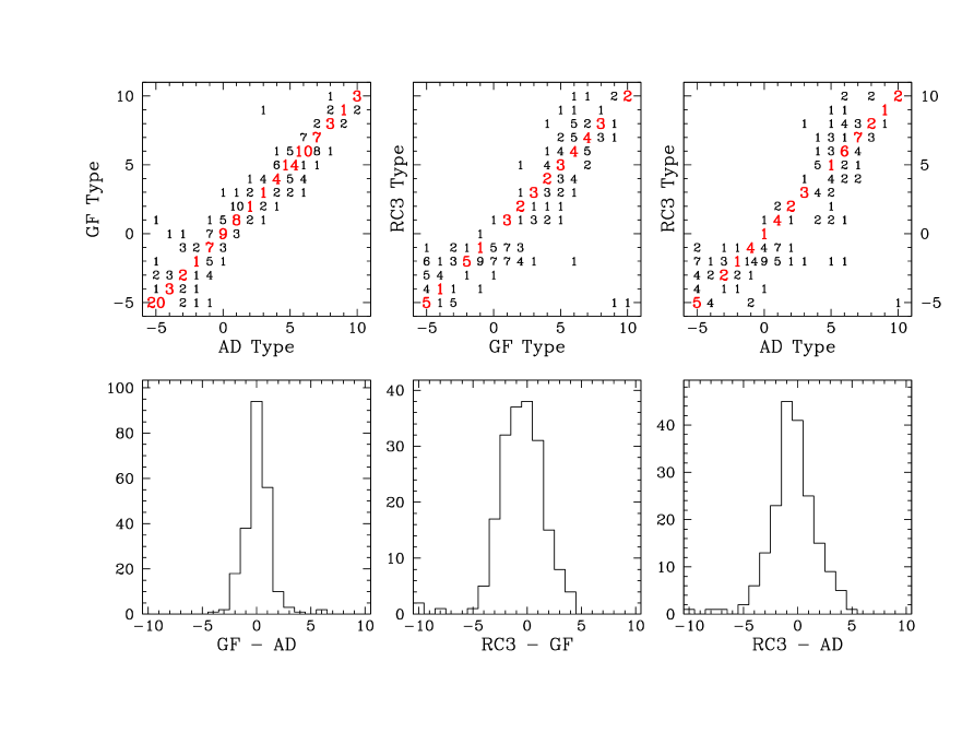
Figure 2: The top panels show the paired comparisons of the classifications from AD, GF and RC3, with the number of galaxies reported in each bin. The bottom panels report the histograms of the differences for each pair of classifiers

The 233 galaxies in the final sample have been independently classified by two of us (AD and GF) using the $T_{RH}$ code adopted in RC3. The top panels of Figure 2 show the paired comparisons of the classifications from AD, GF and RC3, with the number of galaxies reported in each bin. Note that, since in the RC3 and AD databases very uncertain classification has been assigned to 42 and 8 galaxies, respectively (with 5 galaxies having uncertain morphology from both RC3 and AD), the AD-GF, GF-RC3 and AD-RC3 comparisons just rely on 225, 191 and 188 common galaxies, respectively. Note also that compact galaxies, both ellipticals ($T_{RH}$=-6) and irregulars ($T_{RH}$=11), are not present in the selected sample of RC3 galaxies. The histograms of the differences for each pair of classifiers are reported in the bottom panels of Figure 2, while the main statistical quantities of these differences are reported in the first three rows of Table 2. The worse performances of the RC3 classifications with respect to those given by AD end GF can be explained because of the very nature of the RC3 data, which mainly result from compilation and statistical homogenization of different (mostly inhomogeneous) data sources. The fourth and fifth rows of Table 2 report the same quantities relative to the comparisons of the morphological type estimates given by two of us (GF and WJC) for the clusters Abell 1643 and Abell 1878 (z$\sim$0.20 and z$\sim$0.25, respectively; ground based, very good seing imaging taken at the NOT) and for the clusters CL 0024+16 and CL 0939+47 (z$\sim$0.39 and z$\sim$0.41, respectively; WFPC2 imaging from the MORPHS collaboration; Smail et al., 1997). These comparisons are illustrated in Fasano et al. (2000, their Figure 2). Comments about the last row in the Table are given at the beginning of Section 4. From Table 2 the visual morphological classifications turn out not to be biased among each other, the largest average displacement in the table being less than $\Delta T\sim$0.5. Instead, both the $rms$ and the fractions of absolute differences less than 1, 2 and 3 times $T_{RH}$ codes turn out to share relatively wide ranges ($\sigma_{\Delta T}$ from 1.2 to 2.4; $|\Delta$T$|\leq$1 from $\sim$0.53 to $\sim$0.84; $|\Delta$T$|\leq$2 from $\sim$0.79 to $\sim$0.96; $|\Delta$T$|\leq$3 from $\sim$0.91 to $\sim$0.99). It is interesting to note that similar uncertainties on the visual classifications and similar wide ranges in the statistical quantities of the differences were found by the MORPHS collaboration in their morphological catalog of 1857 cluster galaxies at z$\sim$0.5, observed with WFPC2@HST and classified by 4 different human classifiers (Smail et al., 1997, their Figure 1).

Table 2: Comparisons among visual morphological classifications

Comparison	$N_{gal}$	z	Telescope	$<\Delta T>$	$\sigma_{\Delta T}$	$|\Delta T|\leq$1	$|\Delta T|\leq$2	$|\Delta T|\leq$3
AD-GF	225	$\leq$0.03	SDSS	0.076	1.257	0.836	0.960	0.982
GF-RC3	191	$\leq$0.03	SDSS	-0.554	2.374	0.529	0.796	0.932
AD-RC3	188	$\leq$0.03	SDSS	-0.425	2.272	0.569	0.787	0.910
GF-WJC	67	$\sim$0.2	NOT	-0.242	1.348	0.727	0.909	0.985
GF-WJC	207	$\sim$0.5	HST	0.043	1.479	0.773	0.928	0.976
GF-GF	136	0.04$\div$0.07	INT+MPG	-0.072	1.158	0.940	0.976	0.994

3 The MORPHOT tool

Figure 3 shows the flow-chart of MORPHOT. The top and bottom parts of the figure illustrate the calibration and application stages, respectively. Each stage must be read following the direction of the big arrow on the left side. In particular, in the calibration stage, the visual estimates $T_{V}$ (in the MORPHOT system $T_{M}$) are obtained for two samples, each one including $\sim$1000 galaxies, extracted with the same random ctiteria from the WINGS imaging. The first one will be used as a calibration sample for the tool, while the second one will be employed in Section 4 as a test sample in order to assess the performances of MORPHOT. For each galaxy in the calibration sample, (i) the global quantities: size (R), signal-to-noise ratio ($S/N$) and ellipticity ($\varepsilon$) are recorded; (ii) 20 image-based, numerical diagnostics of morphology ($D_{i}$, i=1,…,20) are defined and their values are evaluated. The calibration sample is used to gauge how the diagnostics $D_{i}$ depend on $T_{V}$ and on the global quantities. This allows us to produce a semi-analytical estimator which combines the most effective diagnostics through a Maximum Likelihood technique (ML; see Section 3.3.1 and Appendix B). The same sample is also used as a training set for a Neural Network machine (NN; see Section 3.3.2 and Appendix C), in which the global quantities (R, $S/N$ and $\varepsilon$) and the diagnostics $D_{i}$ are the input quantities and the visual codes $T_{V}$ (in the $T_{M}$ system of Table 1) are the targets. Finally, the NN and the ML estimators are combined to produce the final MORPHOT estimator $T_{M}$.

In the following sub-sections of the present Section the various steps of the MORPHOT tool are described in detail.

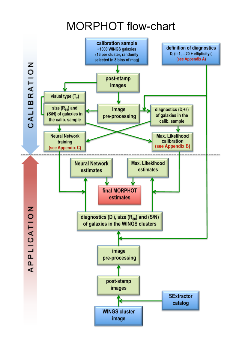
Figure 3: Flow-chart of MORPHOT

3.1 The calibration sample of WINGS galaxies

In the framework of the WINGS project, we have devised the multi-object, automatic surface photometry tool GASPHOT (Pignatelli et al., 2006; D’Onofrio et al., 2011). This tool has been used to perform the detailed surface photometry of 42297 galaxies in the WINGS clusters for which SExtractor (Bertin and Arnouts, 1996) found more than 200 (300) contiguous pixels (threshold area: A_thr) brighter than 1.25 (1.07) times the $rms$ per pixel of the background ($\sigma_{bkg}$) for those images obtained with the WFC@INT (WFI@ESO) ($\sim\mu_{V}$=25.7 for the WINGS survey).

With the aim of providing a sample of galaxies suitable to calibrate MORPHOT, optimizing its performances for WINGS, we decided to randomly extract 16 galaxies per cluster from the WINGS–GASPHOT catalogs, taking care of putting two galaxies in each one of the 8 bins of apparent V magnitude defined as follows: V$\leq$15, 15$<$V$\leq$16, … , 20$<$V$\leq$21, V$>$21. In this way we gathered 1216 WINGS galaxies sampling uniformly the whole range of magnitudes of the GASPHOT–WINGS galaxy sample (see Section 4) and spanning the whole range of observing conditions (background noise and FWHM) of the WINGS optical imaging (see Varela et al., 2009). We decided to remove from this sample those galaxies too close to the edges of the CCDs and/or the very peculiar objects (on-going mergers or quite ill-shapen galaxies). After that, we are left with a final calibration sample of 926 galaxies. All these galaxies have been visually classified by GF according to the $T_{M}$ code shown in Table 1.

It is worth recalling here that the photometry of the WINGS optical survey has been performed on images in which large galaxies and halos of bright stars have been removed after modeling them with elliptical isophotes (see Varela et al., 2009). This allowed us to perform a careful subtraction of the background and estimation of its $rms$ ($\sigma_{bkg}$) even for small galaxies embedded in the halo of the brightest cluster galaxies. Therefore, the WINGS optical catalogs provide, for all galaxies, robust SExtractor determination of the ellipticity ($\varepsilon_{SEx}$) and of the above mentioned threshold area A_thr.

It is also worth mentioning that each individual galaxy is recorded within a square, odd-sized frame of side 3$\times$a_maj, where a_maj corresponds to the semi-major axis (in pixels) of the ellipse with area A_thr and ellipticity $\varepsilon_{SEx}$.

3.1.1 Preliminar image processing

Before running the core-tool of morphological type estimation, for each post-stamp galaxy image of a given sample, MORPHOT automatically performs the refinement of the local background subtraction and the galaxy re-centering. In particular, the central pixel of each galaxy image is made to be coincident with the intensity peak or with the distance-averaged intensity (bari)center, depending on whether the galaxy shows a well defined, dominant light peak (regular shape) or an irregular structure with several local peaks. Moreover, a preliminar processing of the post-stamp galaxy image is performed, which produces two ancillary (and temporary) frames $F_{C}$ and $F_{S}$.

In the frame $F_{C}$ (C: Clean), the possible spurious features (ghosts) and/or those objects (both stars and galaxies) different from the galaxy under analysis are removed by comparing each other the original ($F_{0}$)and the 180^∘ rotated ($F_{180}$) images. In particular, if at a given pixel position the difference $F_{0}$-$F_{180}$ is greater than $n$ times the $rms$ of the pixel values of $F_{180}$ over a box of side = 2$\times$FWHM around the same position, the pixel value in $F_{0}$ is replaced by the corresponding value in $F_{180}$. We have empirically verified that, in our redshift range and with our instrumental set, using $n$=3 allows us to remove satisfactorily most of the unwanted objects without either changing the statistical properties of $F_{0}$ (image texture), or fading the interesting galaxy features, like spiral arms, bars, rings and HII regions.

The frame $F_{S}$ (S: Smooth/Symmetric) is obtained in two steps: first the symmetrization is achieved by averaging (pixel by pixel) $F_{C}$ with its 180^∘ rotated version; then, the median (3$\times$3) and adaptive (Richter et al., 1991, max. block size=11) filters are applied to the symmetrized frame.

It is worth stressing that the evaluation of the morphological diagnostics (see following Sections) is performed on either $F_{C}$ or $F_{S}$, depending on the particular diagnostic. In general, those more specifically linked to the global properties of galaxies (i.e.: different kinds of concentration, etc..) are evaluated on $F_{S}$, while those dealing with pixel-scale structures, local features (clumpiness, diskyness, etc..) and simmetry are evaluated on $F_{C}$. The cleaned image $F_{C}$ is also used to determine the total intensity (I_T, in ADUs) and the final, global geometrical parameters (ellipticity $\varepsilon$ and position angle $\theta$) of the galaxy. These are used in turn to produce a model image $F_{M}$ from the elliptical apertures intensity profile of $F_{C}$, to determine the equivalent radii (in pixels) enclosing 80% of the total galaxy light (R₈₀) and to compute the average signal-to-noise ratio of the galaxy: $S/N$=I_T/($\sigma_{bkg}$A_thr). The global quantities $\varepsilon$, R₈₀ and $S/N$ are used in the calibration procedure of diagnostics (see Section 3.2).

3.2 Morphological diagnostics

Our approach to the automation of morphological classification is a fully empirical one. We do not try to identify an orthogonal set of few, independent and physically pregnant morphological indicators (diagnostics, hereafter), as in the case of the CAS parameter set (Concentration, Asymmetry and Clumpiness; Conselice, 2003) or in the papers by van der Wel (2008) and Scarlata et al. (2007). Rather, we prefer to bet on a large number of diagnostics, no matter if in some cases they are similar among each other, since we postulate that each one of them could potentially be sensitive to some particular morphological characteristic and/or feature of the galaxies. In other words, we decided not to throw out anything a priori and to defer to a later stage the possiblity of giving up some of the diagnostics. As well, we do not try to select the most significant diagnostics by means of statistical techniques, like for instance the Principal Component Analysis (PCA, see Section 3.3). We just test each diagnostic on the field (the test sample, see Section 4), checking whether its addition to the previous (smaller) set of diagnostics improves the tool’s performances (see Section 3.3.1 and Figure 8). Lastly, our diagnostics are not necessarily defined (and conceived) to be independent of the image parameters (photometric depth, noise, pixel size, seeing, etc..). In fact, at least for the time being, we aim to apply MORPHOT just to the WINGS imaging, deferring to a later time the release of a more generally usable version of the tool, where the definition of the diagnostics will be as most as possible independent on the observing material. More explicitly, the calibration of the diagnostics we describe in the next Sections is performed on the WINGS calibration sample defined in Section 3.1 and holds good just for WINGS-like data. For now, applying MORPHOT to imaging data different from WINGS would actually imply a re-calibration of the diagnostics on the new data set.

Up to now we have empirically introduced (and tested) 20 diagnostics. Some of them are not conceptually original, but are usually more simply defined with respect to the similar indicators already present in the literature. Again, we prefer to test a large number of rough diagnostics that are rapidly evaluated, rather than a small set of carefully calibrated (but sometimes hard to compute and not necessarily more efficient) indicators. It is also worth noting that our set of diagnostics is actually open, meaning that additionally devised diagnostics (like, for instance, the spirality analyzers from Naim et al., 1995; Shamir, 2011) can be introduced without changing the structure of the tool. The only limitation we pose for the new diagnostics is that they have to be image-based, thus excluding color- and spectroscopy-based quantities. This is because we think that, in order to have an unbiased picture of the evolution of galaxies in clusters, the information on morphology and stellar population should be kept separate. In Appendix A we present in some detail the definition and the meaning of the 20 diagnostics $D_{i}$ (i=1,…,20). Here we just mention that many of them turn out to be correlated, sometimes strongly so. This is shown in Figure 4 for the calibration sample and it is somehow expected due to our empirical approach.

Figure 4: Mutual correlations among the MORPHOT diagnostics defined in Appendix A.

3.2.1 Diagnostic dependences

Figure 5 illustrates how the 20 morphological diagnostics defined in Appendix A correlate with the visual morphological type for the 926 galaxies of the calibration sample. For the sake of clarity the Y-labels are omitted in the figure and the visual morphological types (integer values) of the calibration galaxies in the southern clusters (304 objects) are shifted by 0.5 upward.

Figure 5: The MORPHOT diagnostics defined in Appendix A vs. visual morphological type for the calibration sample.

Moreover, in Figure 5 the diagnostics $D_{1}$, $D_{7}$, $D_{8}$, $D_{9}$, $D_{10}$, $D_{12}$, $D_{15}$, $D_{19}$ and $D_{20}$ are plotted in logarithmic scale. It is evident from the figure that many diagnostics have quite similar (average) behaviour as a function of the visual morphological type. Still, as explained before, we postulate that even slight differences among diagnostics could in principle help to disentangle different morphological features and we defer the final decision about the diagnostics to be retained to the comparison of the results with the visual classifications. For the moment, it is worth emphasizing the importance of the diagnostics $D_{10}$ and $D_{11}$ in disentangling ellipticals from S0 galaxies. Figure 6 shows that the distributions of these diagnostics for the two morphological types are quite apart. The relative scarcity of non–disky (face-on) S0s in the figure is likely attributable to some cases of face-on S0s which have been visually misclassified as ellipticals. To this concern we note that, with the spatial resolution typical of the WINGS survey, to entirely remove this kind of miss-classification turns out to be almost impossible, even for visual classifications. Actually, Capaccioli et al. (1991) have shown that to distinguish face-on S0s from ellipticals could be a difficult task even for very well resolved galaxies (see Cappellari et al., 2011 for a more radical point of view).

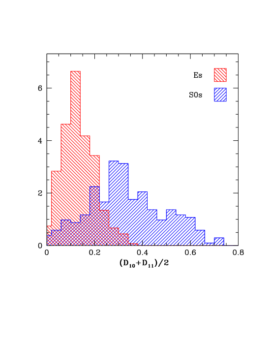
Figure 6: Distribution of the average value of the diskiness diagnostics $D_{10}$ and $D_{11}$ (see Appendix A) for the (visually classified) elliptical and S0 galaxies of the calibration sample

As already stated before, since our aim is to provide morphological classifications of WINGS galaxies, our diagnostics $D_{i}$ are not conceived to be independent on instrumental and observing parameters (pixelsize, seeing, $S/N$, etc..). Figure 7 illustrates how the $D_{i}$ depend on $\log(R_{80}/FWHM)$ and on $\log(S/N)$.

Figure 7: The MORPHOT diagnostics defined in Appendix A vs. $\log(R_{80}/FWHM)$ and $\log(S/N)$.

Instead, no significant dependence of the diagnostics on the apparent ellipticity $\varepsilon$ has been found. To this concern, before describing the techniques we used to extract from our diagnostics univocal estimates of the morphological type, it is worth mentioning that, from now on, we formally include $\varepsilon$ into the set of diagnostics. Therefore, their total number is hereafter assumed to be of 21 ($D_{i}$,i=1,..,20+$\varepsilon$).

3.3 Combining the diagnostics

Having defined the diagnostics $D_{i}$ and tested their dependence on both the visual morphological type ($T_{V}$) and the global quantities R₈₀ and $S/N$, we are left with the difficult task of simultaneously exploiting their capabilities, in order to improve as much as possible the final effectiveness of the tool in recognizing the morphology of galaxies. In other words, we must combine in some (smart) way the 21 diagnostics to obtain a single, final morphological estimator.

Although our empirical approach would drive us to use all the diagnostics (see Section 3.2), we first tried to identify, through the canonical Principal Component Analysis (PCA), an orthogonal transformation converting our diagnostics in a set of uncorrelated variables, smaller than the original set, but still preserving the wealth of morphological information contained therein. However, likely because our diagnostics are not normally distributed, this attempt turned out to be unsuccessful. In fact, running the PCA on our galaxy calibration sample, we just obtained two significant eigenvectors, whose linear combination resulted in an extremely large scatter of the PCA morphological types with respect to the visual estimates. Actually, in Section 3.3.1 (see Figure 8) the number of significant diagnostics is shown to be much larger than two.

Returning to our empirical approach, we used two different techniques, totally independent on each other, in order to obtain the above mentioned combination of the diagnostics and the final, global morphological estimator. It is worth mentioning that both techniques produce morphological type estimates in one digit decimal numbers.

3.3.1 Maximum Likelihood estimator

As outlined at the beginning of Section 3 (see also the flow-chart in Figure 22), the first technique exploits the Maximum Likelihood (ML) statistics to combine the diagnostics. Concisely, after having removed their obvious dependences on the galaxy size (relative to the FWHM) and signal to noise ratio (see Section 3.2.1 and Figure 7), we use the dependence of diagnostics on the visual morphological type in the calibration sample (i.e. the 2D distributions in Figure 5 to estimate the probability that a given value of each diagnostic could come from (be measured for) galaxies of all possible morphological types. Then, for a galaxy with unknown morphology and known (measured) diagnostics, we compute the ML probability (product of the probabilities associated to the diagnostics) as a function of the morphological type $T$ and we assume that the ’true’ morphological type of the galaxy is that providing the largest value of ML. From the function ML($T$), we can also derive the confidence interval of each ML estimate of the morphological type. Details about the MORPHOT-ML technique can be found in Appendix B.

In order to determine how many diagnostics (and which ones) are necessary (and sufficient) to optimize the ML techique, we have first applied the above procedure to all galaxies in the calibration sample using the 21 $D_{i}$ one by one and recording the diagnostic which provides the lowest scatter ($rms$) of the differences between the ML and visual morphological types ($T_{ML}-T_{V}$; hereafter $\Delta T_{ML}$). Then, we have repeated the procedure by adding the remaining 20 diagnostics one by one to the firstly selected diagnostic, and we have again recorded the one which minimizes the above mentioned $rms$ among the 20 couples of diagnostics. We iterated this loop, each time adding one by one the remaining $n$ diagnostics to the (21-$n$) already recorded, while the $D_{i}$ last. Figure 8 illustrates the result of this iteration, showing how the average value and the $rms$ of the $\Delta T_{ML}$ distribution vary as a function of the number $N_{D}$ of diagnostics used to provide the $T_{ML}$ of galaxies in the calibration sample.

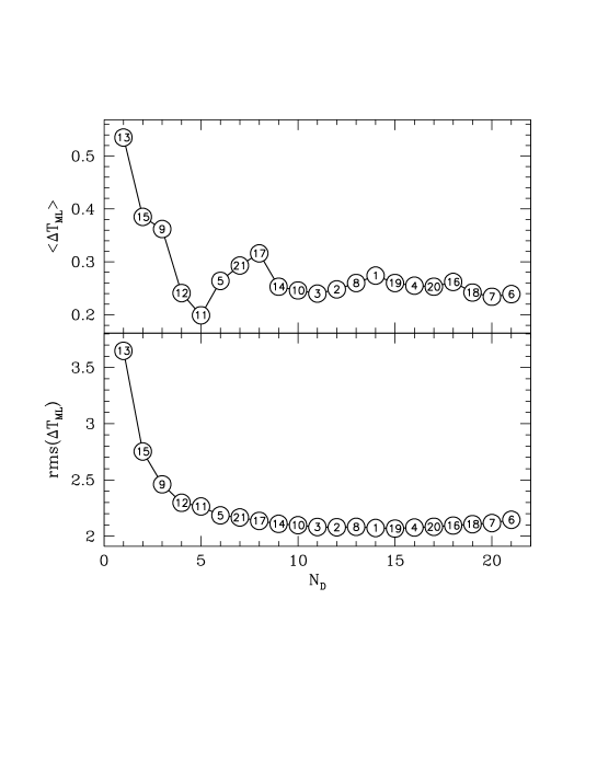
Figure 8: Average value (upper panel) and $rms$ (lower panel) of the differences $\Delta T_{ML}$=($T_{ML}-T_{V}$) as a function of the number of diagnostics ($N_{D}$) used for the ML estimator. The numbers in the open circles identify the diagnostics (see Appendix A) recursively added to the previus ones. The average value and the $rms$ become nearly stable after $N_{D}$=9 and $N_{D}$=11, respectively

The circled numbers in the figure refer to the corresponding diagnostic’s numbers in Appendix A. Figure 8 shows that the average $\Delta T_{ML}$ becomes nearly stable (at $\sim$0.24) after $N_{D}\sim$9, while the $rms$ of the $\Delta T_{ML}$ distribution decreases till $N_{D}\sim$11. It is worth mentioning that, according to the $F$-test for significantly different variances, up to this value of $N_{D}$, the addition of new diagnostics significantly reduces the $rms$, at variance with the (above mentioned) formal result of the PCA. From Figure 8 the diagnostics which turn out to be effective for the ML technique, sorted by decreasing effectiveness, are: $D_{13}$, $D_{15}$, $D_{9}$, $D_{12}$, $D_{11}$, $D_{5}$, $\varepsilon$, $D_{17}$, $D_{14}$, $D_{10}$ and $D_{3}$.

The outlined iterative procedure, aimed at identifying the most effective diagnostics of the ML technique, is clearly an empirical one. For instance, we have chosen to stop the iterations when minimizing the $rms$ ($N_{D}$=11), rather than the average value of $\Delta T_{ML}$, since we consider the minimum $\Delta T_{ML}$ at $N_{D}$=5 to be just a statistical fluctuation due to the finiteness of the test sample. Moreover, we cannot rule out (actually, we consider very likely) the possibility that different combinations of $D_{i}$ coud work better, giving lower values of $rms(\Delta T_{ML})$. Still, testing all possible combinations of the diagnostics was intractable and, we believe, unproductive. Thus, we assume that the morphological types $T_{ML}$ we got using the first eleven effective diagnostics are the best possible ML estimates for the calibration galaxies. Although lacking in a rigorous explanation, we believe the slightly worse $rms$ performance of the tool for $N_{D}>$11 to be due (again) to the finiteness of the test sample, which might induce in the empirical ML procedure a sort of oversampling noise.

The short-dashed lines in Figure 9 connect the median values of $\Delta T_{ML}$ in different bins of $T_{V}$ (upper panel) and the corresponding $rms$ values (lower panel), while the relevant global statistics of the $\Delta T_{ML}$ distribution for the calibration sample are reported in the first row of Table 3.

3.3.2 Neural Network estimator

The second technique we use to combine the morphological diagnostics is based on the classical feed-forward multilayer perceptron Neural Network (NN). Details about the MORPHOT-NN technique can be found in Appendix C. Here we just mention that again the NN morphological type estimates are supplied with confidence intervals, while in this case (at variance with the ML technique) we use as input quantities of the NN machine the whole set of diagnostics ($D_{i}$, i=1,…,20) plus the global quantities $\varepsilon$, $\log(R_{80}/FWHM)$ and $\log(S/N)$. The reason for this choice is explained in Appendix C.

The dot-dashed lines in Figure 9 (blue in the electronic version) connect the median values of $\Delta T_{NN}$ in different bins of $T_{V}$ (upper panel) and the corresponding $rms$ values (lower panel), while the relevant global statistics of the $\Delta T_{NN}$ distribution for the calibration sample are reported in the second row of Table 3. Comparing these values with the corresponding ones relative to the ML technique (first row of the same table) and looking at Figure 9, we conclude that the performances of the NN estimator are significantly better than those of the ML estimator.

3.3.3 The final MORPHOT estimator

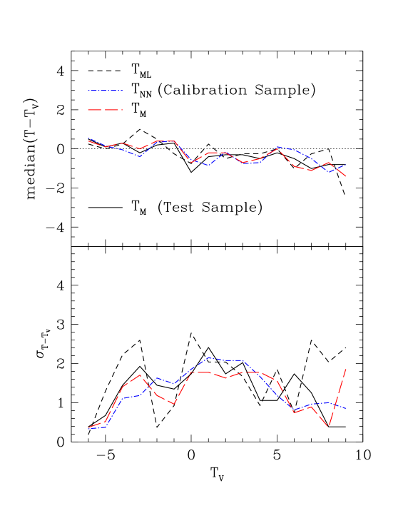
Figure 9: Upper panel: The median values of ($T-T_{V}$) in different bins of $T_{V}$ are connected for the estimators $T_{ML}$ (short-dashed line), $T_{NN}$ (dot-dashed line, blue in the electronic version) and $T_{M}$ (long-dashed line, red in the electronic version) obtained running MORPHOT on the calibration sample. The full (black) line illustrates the behaviour of the $T_{M}$ estimators obtained running MORPHOT on the test sample (see Section 4). Lower panel: The $rms$ of ($T-T_{V}$) in different bins of $T_{V}$ for the estimators $T_{ML}$, $T_{NN}$ and $T_{M}$ in the case of the calibration sample. The meaning of the different lines are as in the upper panel. The full (black) line refers to the $T_{M}$ estimator in the case of the test sample.

As already pointed out at the beginning of Section 3.3, the Maximum Likelihood and the Neural Network provide conceptually and technically different approaches to the problem of combining the morphological diagnostics. Therefore, the MORPHOT estimators produced by the two techniques ($T_{ML}$ and $T_{NN}$) should be independent on each other and the $rms$ of their difference should roughly be the square root of the sum of their variances with respect to $T_{V}$ ($rms[T_{ML}-T_{NN}]\sim$2.55). Actually, elementary numerical simulations show that the particular density distribution of $T_{V}$ makes the real $rms$ lower than the above theoretical value, in agreement with the value we found in the calibration sample ($rms$=2.05, see last row in Table 3).

Once the mutual independence of the two estimators has been checked, the last step of the MORPHOT flow-chart (see Figure 3) is the evaluation of the final morphological type estimator $T_{M}$, which is simply defined as the average value of the two independent estimators: $T_{M}$=($T_{ML}+T_{NN}$)/2. Similarly, the lower and upper limits of the confidence interval of $T_{M}$ are obtained by averaging the lower and upper confidence limits of $T_{ML}$ and $T_{NN}$, respectively.

The long-dashed lines in Figure 9 (red in the electronic version) connect the median values of $\Delta T_{M}$ in different bins of $T_{V}$ (upper panel) and the corresponding $rms$ values (lower panel), while the relevant global statistics of the $\Delta T_{M}$ distribution for the calibration sample are reported in the third row of Table 3.

Comparing these values with the corresponding ones relative to the ML and NN techniques (first two rows of the same table), we should conclude that the global performances of the NN estimator are even better than those of the final MORPHOT estimator, thus making convenient to adopt $T_{NN}$ alone to optimize the performances of MORPHOT. Still, just because of the above mentioned mutual independence of the ML and NN estimators, we are inclined to believe that their combination could in any case provide more stable results, each technique possibly compensating the biases of the other one. Actually, from the upper panel of Figure 9, the biases of the $T_{M}$ and $T_{NN}$ estimators in different bins of $T_{V}$ have quite similar sizes, while the scatter of the $T_{M}$ estimator along the $T_{V}$ sequence (long-dashed, red line in the lower panel) turns out to be more stable than in the case of the $T_{NN}$ estimator (dot-dashed, blue line in the same panel). Therefore, we decided to adopt $T_{M}$ as final MORPHOT estimator.

It is worth noting that all the estimators tend to be biased towards later and earlier morphological types for the early and late visual types, respectively. However, this is expected (and in some sense obvious) because of the one-sided error distribution of galaxies close to the limits of the available range of visual morphological types.

4 Testing the performances of MORPHOT

As mentioned in Section 3, the test galaxy sample has been extracted from the V-band WINGS imaging using the same (random) criteria described in Section 3.1 for the calibration sample. Again, we removed from the initial sample of 1216 galaxies those objects too close to the edges of the CCDs and/or the very peculiar objects (on-going mergers or quite ill-shapen galaxies), being left with a final sample of 979 objects, which have been visually classified by GF according to the $T_{M}$ code exemplified in Table 1. It is worth noting that 136 (mostly bright) galaxies turned out to be in common between the calibration and the test samples. Since the classifications of the two samples (both from GF) are independent from each other, these galaxies have been used to estimate the internal consistency of the visual classifications from GF. The main statistical indicators of this comparison are reported in the last row of Table 2. They show that significant differences can be found even comparing among each other the morphological classifications provided by the same human classifier, for the same galaxy sample, but at different times.

For all the galaxies in the test sample, we have computed the global quantities ($\varepsilon$, $R_{80}$ and $S/N$) and the MORPHOT diagnostics $D_{i}$ and we have obtained the Maximum Likelihood ($T_{ML}$), the Neural Network ($T_{NN}$) and the final ($T_{M}$) MORPHOT estimators of the morphological type.

Table 3: Comparisons between visual morphology and MORPHOT Type for both the calibration and the test samples. The last row refers to the mutual comparison between $T_{ML}$ and $T_{NN}$.

$\Delta T$	Sample	$<\Delta T>$	$\sigma_{\Delta T}$	median($\Delta T$)	$|\Delta T|\leq$1	$|\Delta T|\leq$2	$|\Delta T|\leq$3
$T_{ML}-T_{V}$	CALIB	0.24	2.08	0.00	0.616	0.778	0.867
$T_{NN}-T_{V}$	CALIB	-0.05	1.47	0.10	0.656	0.875	0.951
$T_{M}-T_{V}$	CALIB	0.01	1.56	0.10	0.640	0.832	0.925
$T_{M}-T_{V}$	TEST	-0.06	1.72	0.00	0.631	0.803	0.885
$T_{ML}-T_{NN}$	CALIB	0.29	2.05	0.10	0.522	0.754	0.865

In the fourth row of Table 3 we report the relevant statistical quantities of the comparisons between visual and MORPHOT classifications for the test sample.

From Tables 2 (rows 1, 4 and 5) and 3 (rows 3 and 4) and from Figure 9 one can derive the following remarkable conclusions: (i) for the calibration sample the scatter of the $T_{M}$ estimator with respect to the visual classifications turns out to be quite comparable to (sometimes better than) the scatter reported in Table 2 among visual types provided by different experienced human classifiers; (ii) for the test galaxy sample, the above mentioned scatter just marginally increases with respect to the previous case, still remaining quite competitive with respect to the average scatter among visual classifications.

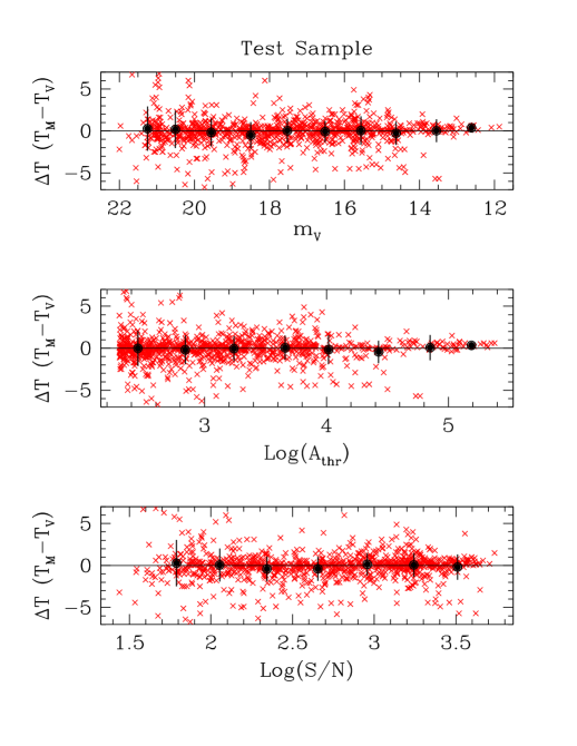
Figure 10: Dependence of the difference ($T_{M}-T_{V}$) on apparent magnitude (upper panel), threshold area (middle panel) and signal to noise ratio (bottom panel) for the test sample. The big, full dots and the corresponding error bars illustrate the average values ond the $rms$ in each bin.

Figure 10 illustrates how the differences $\Delta T_{M}$=$T_{M}$-$T_{V}$ (average value and scatter) behave as a function of apparent magnitudes, threshold areas and the S/N ratios of galaxies in the test sample. As might be expected, the scatter of $\Delta T_{M}$ increases (from $\sim$0.7 to $\sim$2) at decreasing the threshold area (in pixels) and the apparent luminosity of galaxies. Instead, no dependence of the scatter on $S/N$ is found.

Figure 11: Comparison between visual and MORPHOT ’broad’ morphological classes for the galaxies of the MORPHOT test sample. At the top of the 2D-bins the percentages of the visual classes (Es, S0s, early spirals [SpE], late spirals [SpL] and irregulars) falling in different bins of the MORPHOT classification are reported. Similarly, the percentages of the MORPHOT classes falling in different bins of the visual classification are reported in the right side of the 2D-bins. Finally, on the top (columns) and on the right (rows) of the plot, we report the total number of galaxies in each ’broad’ class of the visual and MORPHOT estimates, respectively.

Figure 11 illustrates the comparison between the visual and the final ($T_{M}$) morphological classifications of the galaxies in the test sample. In this case the comparison is made in ’broad’ bins of morphology, where the ’broad’ classes are conventionally defined as follows: Ellipticals (E), for $T<$-4; Lenticulars (S0), for -4$\leq T\leq$0; Early-Spirals (SpE), for 0$<T\leq$4; Late-Spirals (SpL), for 4$<T\leq$7; Very Late-Spirals and Irregulars (Irr), for $T>$7. Note that we have included the cD galaxies in the broad class E. This is because MORPHOT tends to classify as cDs ($T$=-6) some among the brightest and largest ellipticals in the test sample. Note also that we have included in the S0 ’broad’ class both the galaxies classified E/S0 ($T$=-4) and those classified S0/a ($T$=0).

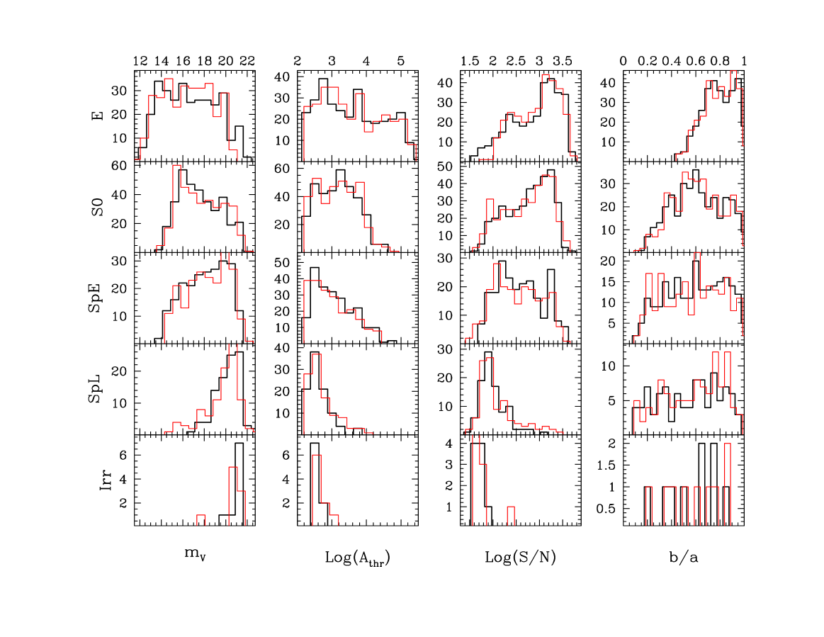
Figure 12: The distributions of apparent magnitudes (V-band), threshold areas (pixels), signal to noise ratios and axial ratios for different ’broad’ morphological classes (Es, S0s, early spirals [SpE], late spirals [SpL] and irregulars) in the WINGS test galaxy sample. The thick line histograms refer to the visual morphological types ($T_{V}$), while the thin line histograms (red in the electronic version of the paper) illustrate the distributions for the MORPHOT estimates ($T_{M}$)

Finally, Figure 12 illustrates in more detail the results already shown in the previous two figures and compares, for different ’broad’ morphological classes, the distributions of apparent magnitude, threshold area, signal to noise and axial ratios obtained from the visual (thick lines) and MORPHOT (thin lines, red in the electronic version of the paper) estimates of the test galaxy sample.

Figures 11 and 12 show that, besides mimiching the statistics $<\Delta T>$ and $\sigma_{\Delta T}$ of the comparison between human classifiers (see Tables 2 and  3), the automatic morphological types are able to fairly reproduce the global morphological fractions of the visual types (Figure 11), as well as the fractions binned according to several observed quantities (Figure 12). In particular, Figure 11 shows that, in spite of the wide range of $T_{M}$ corresponding to each bin of $T_{V}$ (and viceversa), the global fractions of visually classified E and S0 galaxies in the test sample are almost exactly reproduced by the MORPHOT types.

5 Applying MORPHOT to the WINGS clusters

The bottom part of Figure 3 illustrates the flow-chart relative to the application of MORPHOT to the WINGS clusters.

Concisely: (i) for the galaxy catalog of a given WINGS cluster, post-stamp frames of the galaxies to be classified are extracted from the original WINGS imaging; (ii) for each galaxy, the global quantities (R₈₀, $S/N$ and $\varepsilon$) and the diagnostics $D_{i}$ are evaluated and the (independent) NN and ML estimators of the morphological type are produced, each one with the proper confidence interval; (iii) the final MORPHOT estimator is obtained by averaging the NN and ML estimators.

According to Varela et al. (2009), the WINGS optical (B,V) imaging provides photometric and geometric description of 400140 galaxies in 77 clusters ($\sim$5200 galaxies per cluster, on average). As already mentioned in Section 3.1, for about one tenth of them (42297 galaxies: those with threshold area greater than 200/300 pixels for images from WFC@INT/WFI@ESO) the surface photometry has been performed with GASPHOT (Pignatelli et al., 2006). We use the GASPHOT-WINGS catalogs as input galaxy sample to perform the morphological analysis of WINGS galaxies with MORPHOT.

5.1 The WINGS morphological catalogs

The total number of galaxies in the GASPHOT catalogs is 42,297. We removed from the sample those galaxies for which the Sersic index provided by GASPHOT coincides with the boundaries of the allowed range (0.5$-$8), which usually indicates that the fitting procedure was unsuccessful (Pignatelli et al., 2006). In this way we are left with 39651 galaxies in the fields of the WINGS clusters. For 527 galaxies (1.3% of this sample) MORPHOT produced unreliable results since it was not able to compute some of the diagnostics (fuzzy/faint objects). The remaining 39124 galaxies have been processed by MORPHOT, which provides $T_{ML}$, $T_{NN}$ and $T_{M}$ estimates of the morphological types, together with the corresponding confidence intervals $T^{min}$ and $T^{max}$.

We have very quickly checked on the WINGS imaging the MORPHOT classification of the bright galaxies (mostly brighter than $V$=18) and in 426 cases ($\sim$1% of the total sample; $\sim$5% of the checked sample) we have modified the final classification since it was clearly wrong. Profiting from this visual inspection procedure, we have also manually added to the catalogs the morphological types of 799 bright galaxies (again mostly brighter than $V$=18), close to the borders of the frames or close to bright stars, which had been discarded ’a priori’ by the GASPHOT and MORPHOT tools. After this manual intervention, the total number of WINGS galaxies for which we provide the final morphological type estimate ($T_{F}$) is 39923. Among them, 2963 are visual estimates ($T_{V}$). This latter number includes the 926 galaxies of the Calibration Sample, the 979 galaxies of the Test Sample (136 of them turned out to be in common with the calibration sample; see Section 4), the 426 galaxies whose classification has been modified after visual check (31 of them turned out to be in common with the test sample) and the 799 galaxies manually added to the catalogs. The full MORPHOT catalog of WINGS galaxies is available from the “Centre de Données Astronomiques de Strasbourg” (CDS) using the ViZiER Catalogue Service. Table 4 show the first few records of the catalog.

Table 4: Sample rows of the MORPHOT WINGS catalog

WINGS_ID	Cluster	$T_{ML}$	$T_{ML}^{min}$	$T_{ML}^{max}$	$T_{NN}$	$T_{NN}^{min}$	$T_{NN}^{max}$	$T_{M}$	$T_{M}^{min}$	$T_{M}^{max}$	$T_{V}$	$T_{F}$
WINGSJ103833.76-085623.3	A1069	3.1	-0.3	4.6	5.9	1.6	8.6	4.5	2.7	6.3		4.5
WINGSJ103834.09-085719.2	A1069	4.3	3.0	5.2	4.1	0.5	7.7	4.2	3.7	4.7		4.2
WINGSJ103834.13-085030.4	A1069	-5.0	-5.0	-4.7	-5.1	-6.0	-4.4	-5.0	-5.5	-4.5		-5.0
WINGSJ103835.85-084941.0	A1069	1.8	-0.1	3.7	-0.2	-3.5	3.9	0.8	-0.5	2.1		0.8
WINGSJ103835.89-085031.5	A1069	-1.5	-3.5	0.5	-3.2	-5.1	-1.4	-2.3	-3.4	-1.2		-2.3
WINGSJ103836.38-083614.8	A1069	3.8	1.6	4.2	5.0	0.2	8.9	4.4	3.6	5.2		4.4
WINGSJ103836.95-085300.8	A1069	-5.0	-5.0	-4.5	-5.9	-6.0	-5.1	-5.5	-5.5	-4.5	-5.0	-5.0
WINGSJ103837.15-085753.4	A1069	3.2	0.2	5.3	4.4	1.1	7.9	3.8	2.5	3.5	3.0	3.0
WINGSJ103837.48-083717.2	A1069	-1.9	-3.8	-0.0	-3.4	-4.8	-1.6	-2.6	-3.6	-1.6		-2.6
WINGSJ103837.93-084940.5	A1069	-5.0	-5.0	-4.5	-0.9	-5.2	3.7	-3.0	-5.0	-1.0		-3.0
WINGSJ103838.65-084938.3	A1069	-2.4	-3.5	-1.1	0.5	-3.2	4.8	-0.9	-2.4	0.6		-0.9
WINGSJ103839.63-084742.6	A1069	2.0	-2.3	2.7	-1.4	-3.9	0.9	0.3	-1.5	2.1		0.3
WINGSJ103840.54-085041.1	A1069	-3.0	-4.6	0.8	-4.0	-5.9	-1.4	-3.5	-4.3	-2.7		-3.5
WINGSJ103840.85-085046.5	A1069	-4.9	-3.8	-2.3	-5.3	-6.0	-4.5	-5.1	-5.6	-4.6		-5.1
WINGSJ103841.43-085521.6	A1069	-3.7	1.5	3.3	6.0	0.9	9.4	1.1	-3.8	6.0		1.1
WINGSJ103841.63-085528.6	A1069	-4.8	-3.5	-2.7	-3.5	-5.5	-1.4	-4.2	-4.9	-3.5		-4.2
WINGSJ103842.12-083557.8	A1069	-5.0	-5.0	-4.1	0.5	-4.5	6.0	-2.3	-5.0	0.4		-2.3
WINGSJ103843.03-085602.8	A1069	-5.0	-5.0	-4.3	-4.9	-5.8	-3.8	-5.0	-5.5	-4.5		-5.0
WINGSJ103844.19-085609.3	A1069	0.5	-2.1	0.7	-1.9	-3.8	0.4	-0.7	-2.0	0.6		-0.7
WINGSJ103844.58-084601.1	A1069	4.5	3.4	5.4	5.3	1.2	8.4	4.9	4.3	5.5		4.9
WINGSJ103845.53-085341.2	A1069	3.1	1.4	4.0	-3.1	-5.3	-0.5	0.0	-3.1	3.1		0.0
WINGSJ103845.73-084021.9	A1069	0.3	-1.6	0.6	-3.8	-6.0	1.9	-1.7	-3.8	0.4		-1.7
WINGSJ103846.39-084530.6	A1069	-3.9	-4.8	-0.9	-2.3	-4.8	0.7	-3.1	-4.5	-3.5	-4.0	-4.0
WINGSJ103846.47-084226.0	A1069	-0.9	-2.6	0.8	0.7	-1.7	2.9	-0.1	-1.2	1.0		-0.1
WINGSJ103847.59-084631.3	A1069	-1.4	-2.1	-0.2	-5.5	-6.0	-4.3	-3.5	-5.6	-1.4		-3.5
WINGSJ103848.08-085044.8	A1069	-5.0	-5.0	-4.5	-3.9	-4.6	-2.9	-4.4	-5.0	-3.8		-4.4
WINGSJ103848.30-084259.9	A1069	-0.1	-2.2	1.1	0.3	-1.6	2.3	0.1	-0.5	0.7		0.1
WINGSJ103850.17-085336.6	A1069	-2.7	-0.5	2.2	2.3	-1.5	6.3	-0.2	-2.7	2.3		-0.2
WINGSJ103850.35-084804.5	A1069	-2.8	-3.3	-0.8	-0.5	-4.0	3.8	-1.7	-3.0	-0.4		-1.7

5.2 External comparisons

In order to provide an external check of the goodness of our automated classifications, we have searched the literature for visually classified galaxy samples having objects in common with our WINGS-MORPHOT sample. We only found three possible data samples that could be usable for our purpose, all of them concerning the SDSS galaxies: Fukugita et al. (2007), Nair et al. (2010) and Lintott et al. (2011, Galaxy Zoo). By cross-matching these samples with our catalog, we found that the objects in common are 18, 79 and 2110, respectively. However, the potentially most sizeable comparison sample (Galaxy Zoo) turns out to be practically useless, since it just provides the binary information Elliptical/Spiral (no S0 classification). Moreover, while the morphological resolution of the classification system adopted by Nair et al. (2010) is comparable (not equal) to the MORPHOT resolution, the Fukugita et al. (2007) system only enables us to compare the ’broad’ morphological classes.

Figure 13: Comparison between MORPHOT and literature morphological types (see the comments in the text). Left panel: number of galaxies in the different bins of ’broad’ morphological class for the sample of 18 WINGS-MORPHOT galaxies in common with Fukugita et al. (2007). Right panel: the MORPHOT vs. Nair et al. (2010) morphological types for the 79 common galaxies.

Figure 13 illustrates the comparison of the MORPHOT morphological types with the Fukugita et al. (2007) and Nair et al. (2010) classifications (left and right panel, respectively). In both cases the MORPHOT results tend to be slightly shifted towards earlier types with respect to the visual estimates. However, in spite of the small number of cross-matched galaxies and of the different classification systems, the agreement between the MORPHOT automated morphological types and the visual estimates from the literature looks satisfactory. In particular, the average value and the scatter of the difference ($T_{M}$-$T_{Nair+}$) turn out to be -0.4 and 1.4, respectively, to be compared with the corresponding values given in Tables 2 and 3.

5.3 Morphological properties of the WINGS clusters

This section outlines the main statistical properties of the galaxy morphology in the WINGS clusters. More detailed and exhaustive analyses about this topic will be presented in a few forthcoming papers. Here we just illustrate some general morphological trend emerging from WINGS-MORPHOT catalogs.

Figure 14 illustrates the distribution of the MORPHOT types ($T_{M}$) in the fields of the WINGS clusters. The contribution of the general field to the different morphological types has been estimated in two independent ways. First, we have counted galaxies in the general field of the Padova Millennium Galaxy and Group Catalogue (PM2GC; Calvi et al., 2011), for which we have obtained MORPHOT classifications. Second, we have estimated the fraction of cluster members in the WINGS fields using the spectroscopic completeness and membership functions derived for the WINGS survey by Cava et al. (2009). In the first case (upper panel of Figure 14) we can confidently assume the PM2GC survey to be nearly complete down to $V_{lim}$=18, while the selection of the WINGS spectroscopic sample has been extended down to $V\sim$20 (central panel of the figure). In this case, the completeness function is mainly determined by time allocation and fiber crowding problems. Moreover, the spectroscopic WINGS survey only includes a subsample of the original WINGS cluster sample (48 over 77). In spite of these differences, the distributions of the MORPHOT types in the WINGS clusters, obtained applying to the WINGS-MORPHOT catalogs the two (independent) statistical corrections for membership, turn out to be remarkably consistent (see the bottom panel in the same figure). The consistency is confirmed even if we use $V_{lim}$=18 also for the membership correction based on the spectroscopic completeness.

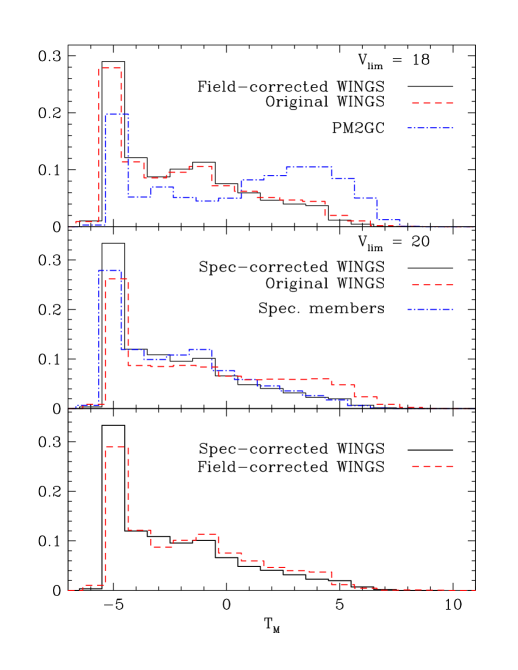
Figure 14: Distribution of MORPHOT types in the WINGS clusters. Upper panel: The distributions for the uncorrected WINGS sample, for the general field sample (from PM2GC; Calvi et al., 2011) and for the field-corrected WINGS sample up to the apparent magnitude V=18 are illustrated by dashed, dot-dashed and full line histograms, respectively. Middle panel: The distributions for the uncorrected WINGS sample, for the spectroscopic WINGS members and for the WINGS sample corrected with the spectroscopic copleteness and membership functions derived from Cava et al. (2009) are illustrated by dashed, dot-dashed and full line histograms, respectively. In this case a deeper magnitude limit (V=20) has been used (see text). Bottom panel: Comparison between the field-corrected and the spectroscopy-corrected distribution of the MORPHOT types in the WINGS clusters. In spite of the different magnitude limits adopted for the statistical corrections, the two distributions turn out to be quite consistent each one another. The same happens if we adopt for the spectroscopic membership correction the same magnitude limit we used for the statistical filed (PM2GC) correction ($V_{lim}$=18).

Adopting the ’broad’ morphological classes conventionally defined in Section 4, we find that ellipticals, S0s and spiral galaxies constitute $\sim$33%, 44% and 23% of the whole galaxy population in the WINGS clusters. It is worth to note that these morphological fractions are slightly different from those found in Poggianti et al. (2009). The discrepancy mostly concerns the E/S0 ratio and is due to the combined effects of two factors: (i) the limit of 0.6$\times R_{200}$ adopted for the clustercentric distance in Poggianti et al. (2009); (ii) the behaviour of the E/S0 ratio as a function of the clustercentric distance. Figure 15 illustrates the point, showing the morphological fractions as a function of the clustercentric distance before and after correction for field contamination (right and left panels, respectively). Note the prevalence of Es in the inner cluster regions, which is responsible for the different E/S0 ratio found in Poggianti et al. (2009). Note also that the field correction does not influence this ratio up to $\sim$0.5$\times R_{200}$, mostly operating on the S0/Early-Spirals fraction in the external part of the clusters.

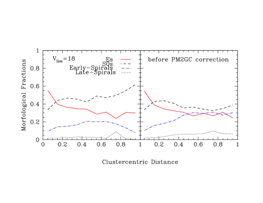
Figure 15: Morphological fractions as a function of the clustercentric distance (in $R_{200}$ units) for the WINGS galaxies before and after correction for field contamination. The general field morphological fractions in different bins of apparent V-band magnitude have been derived from the PM2GC sample (Calvi et al., 2011) using the magnitude limit V=18.

Figure 16 shows the distributions of the projected ellipticities in the WINGS-MORPHOT catalogs for different ’broad’ morphological classes. In this case we do not try to correct for cluster membership, since we just aim to check the plausibility of the distributions, also in comparison with the literature. To this concern, the ellipticity distribution of elliptical galaxies in Figure 16 turns out to be in perfect agreement with Fasano et al. (1991, see also , ), while for S0s and Early-Spirals the peaks of the distributions are slightly shifted towards lower values of the ellipticities with respect to the corresponding distributions in Fasano et al. (1993). However, this is not surprising, since our flattenings come from global, single component (Sersic) fitting of the galaxy image (GASPHOT), while the axial ratios in Fasano et al. (1993) refer to the outer isophotes (essentially the disk components). The peculiar ellipticity distribution of Late-Spirals is due to the inclusion in this ’broad’ class of the irregular objects, which could be intrinsically less flattened than disk galaxies.

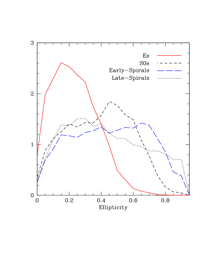
Figure 16: Ellipticity distributions of WINGS galaxies for different ’broad’ morphological classes. The Irregular galaxies have been included in the Late-Spirals (see comments in the text). No correction for field contamination has been applied.

Figure 17 show the distributions of the (B-V) color for the spectroscopically confirmed members in the WINGS-MORPHOT catalogs and for the different ’broad’ morphological classes. Note the remarkable similarity and the small, but statistically significant shift between the distributions of E and S0 galaxies. Note also the bi-modal color distribution of the Late-Spirals(+Irr) galaxies.

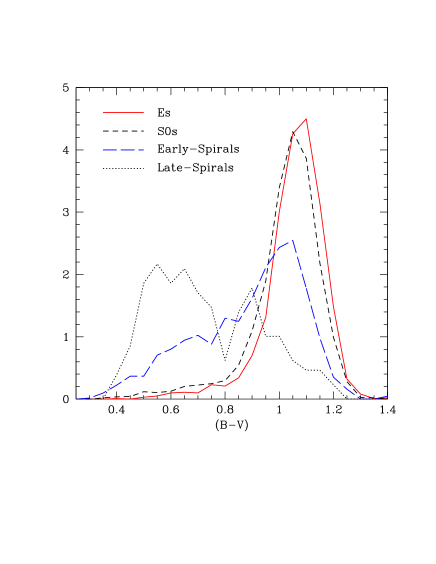
Figure 17: (B-V) color distributions of spectroscopically confirmed WINGS cluster members for different ’broad’ morphological classes. The Irregular galaxies have been included in the Late-Spirals (see comments in the text).

Finally, in Figure 18 we present the distribution of the Sersic index $n$ for the different ’broad’ morphological classes. Again, in this case we do not try to correct for cluster membership. The Sersic indices come from our WINGS-GASPHOT catalogs. As already mentioned in Section 1, even though a correlation between these n and the morphological type exists, it is weak and it shows a high degree of degenaracy, especially for early-type galaxies (see the distributions for bright and faint Es).

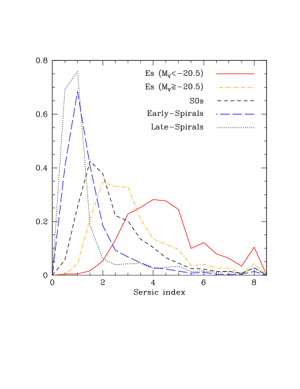
Figure 18: Sersic index distributions of WINGS galaxies for different ’broad’ morphological classes. Elliptical galaxies have been divided in bright ($M_{V}<$-20.5) and faint ($M_{V}\geq$-20.5) Es, while the Irregular galaxies have been included in the Late-Spirals (see comments in the text). No correction for field contamination has been applied.

6 Summary

In this paper we have presented the morphological classification of $\sim$40000 galaxies in the fields of 76 nearby clusters from the WINGS optical (V-band) survey. The morphological types have been estimated automatically, using the purposely devised tool MORPHOT, whose description takes up a substantial part of the paper. It combines a large set (21) of diagnostics, easily computable from the digital cutouts of galaxies, producing two different estimates of the morphological type based on: (i) a semi-analytical Maximum Likelihood technique; (ii) a Neural Network machine. The final, averaged estimator has been tested over a sample of $\sim$1000 visually classified WINGS galaxies, proving to be almost as effective as the ’eyeball’ estimates themselves. In particular, at variance with most existing tools for automatic morphological classification of galaxies, MORPHOT has been shown to be able to distinguish between ellipticals and S0 galaxies with unprecedented accuracy. Even though its basic methodology is robust for any set of digital images of similar spatial resolution and dynamic range, MORPHOT is presently calibrated and fine-tuned to provide reliable morphologies of WINGS galaxies alone. Adjustments of the calibration are required (and are actually in progress) to make the tool more generally usable. The WINGS-MORPHOT catalog has been exploited here just to illustrate the distributions of some relevant photometric and structural properties of galaxies in the WINGS clusters. In a few forthcoming papers of the WINGS series, we plan to perform more detailed statistical analyses involving the morphology of cluster galaxies. In particular, besides the classical morphology–density and morphology–clustercentric distance relations, we will exploit the WINGS spectroscopic information (Cava et al., 2009; Fritz et al., 2007, 2011; Hansson et al., 2011) to study how galaxy morphology correlates with star formation rate and history at different clustercentric distances.

Appendix A The current set of diagnostics: definitions

Here we present in some detail the definition and the meaning of the 20 diagnostics $D_{i}$ (i=1,…,20) we devised up to now. The first nine of the following diagnostics are actually already present in the literature, although sometimes in slightly different forms. We will refer to the original papers for details about their definitions. Instead, the remaining eleven diagnostics are presented here for the first time. Hereafter, in the definition of diagnostics, we use just the pixels above the threshold value (2$\sigma_{bkg}$) and far from the galaxy center more than the image FWHM.

A.1 Diagnostics already present in the literature

$D_{1}$: Sersic index of the luminosity profile.

Given the FWHM, this diagnostic is evaluated on the image $F_{S}$ according to the prescriptions given in Trujillo et al. (2001, ; Section 4 therein), making use of the previously extracted elliptical aperture intensity profile of the galaxy (see Section 3.1.1);

$D_{2}$: Luminosity-ranked Concentration index.

Again from the image $F_{S}$ and from the elliptical aperture intensity profile, this diagnostic is evaluated as the fraction of the total intensity coming from the 30% brightest pixels;

$D_{3}$: Distance-ranked Concentration index.

Similar to the previous one, but defined as the fraction of the total intensity coming from the 30% pixels closest to the galaxy center (in units of elliptical distances). Note that more elaborated versions of the Concentration indices can be found in Graham et al. (2001), Conselice (2003) and Yamauchi et al. (2005);

$D_{4}$: Luminosity-ranked Gini Coefficient.

Following Abraham et al. (2003) and Lotz et al. (2004), inside the square whose sides coordinates are the fraction of galaxy pixels and the fraction of the total counts (square area $\equiv$ 1), we define this diagnostic as the area between the diagonal of the square and the galaxian Lorentz curve (i.e.: the rank-ordered cumulative distribution function of the pixel counts). For this diagnostic and for the following one we use the image $F_{S}$;

$D_{5}$: Distance-ranked Gini Coefficient.

Similar to the previous one, but in this case the pixels are ranked in ascending order of elliptical distance from the galaxy center;

$D_{6}$: Second-order moment of light.

Following Lotz et al. (2004), we define this diagnostic as the second-order moment of the brightest 20% pixels of the image $F_{S}$, normalized to the same moment computed over the whole galaxy area;

$D_{7}$: Asymmetry.

For this diagnostic we use the image $F_{C}$ and we adopt the definition given in Conselice (1997, ; normalized square counts of the difference between the original and the 180^∘ rotated image), with the improvements suggested in Conselice et al. (2000, ; see their Section 3.4) about the preliminar image processing (careful centering) and the handling of the uncorrelated noise;

$D_{8}$ and $D_{9}$: Clumpiness.

The diagnostic $D_{8}$ is defined according to Conselice (2003, see equation 2 therein), including in the sum just the pixels with counts above the threshold (2$\sigma_{bkg}$) and far from the galaxy center more than the image FWHM. The second clumpiness diagnostic ($D_{9}$) is similar to the previous one. However, in order to further enhance high-frequency features, in this case the model image $F_{M}$ defined in Section 3.1.1 is subtracted from the galaxy image $F_{C}$, instead of the gauss-smoothed version of the image itself;

A.2 New Diagnostics

The following morphological diagnostics are presented here for the first time. They all are computed on the frame $F_{C}$, again using just the pixels above the threshold (2$\sigma_{bkg}$) and far from the galaxy center more than the image FWHM. We recall (see Section 3.1) that $F_{C}(i,j)$ is a square matrix, whose size (N) must be an odd number.

$D_{10}$ and $D_{11}$: Diskyness.

The difference between the galaxy image $F_{C}$ and the model image $F_{M}$ (residual image; hereafter $F_{R}$) is used to devise two new diagnostics related to the shape of the galaxy isophotes ($a_{4}>0\equiv$disky, $a_{4}<0\equiv$boxy; Bender and Moellenhoff, 1987). The first diagnostic is defined as:

$$D_{10}=(<F_{R1}>-<F_{R2}>)/<|F_{R}|>$$

where $<F_{R1}>$ and $<F_{R2}>$ are the average counts of $F_{R}$ in the equal-area sectors of the above defined model-ellipse marked respectively with 1 and 2 in the bottom panel of Figure 19. In the formula, the quantity $<|F_{R}|>$ is a normalization factor representing the average value of the (absolute) counts of $F_{R}$ over the whole model-ellipse (apart from the inner circle of radius=FWHM). Clearly, $D_{10}$ tend to be positive in galaxies with disk-shaped isophotes, since in this case the residuals in the two sectors marked 1 tend to be greater (darker in the figure) than those in sectors marked 2.

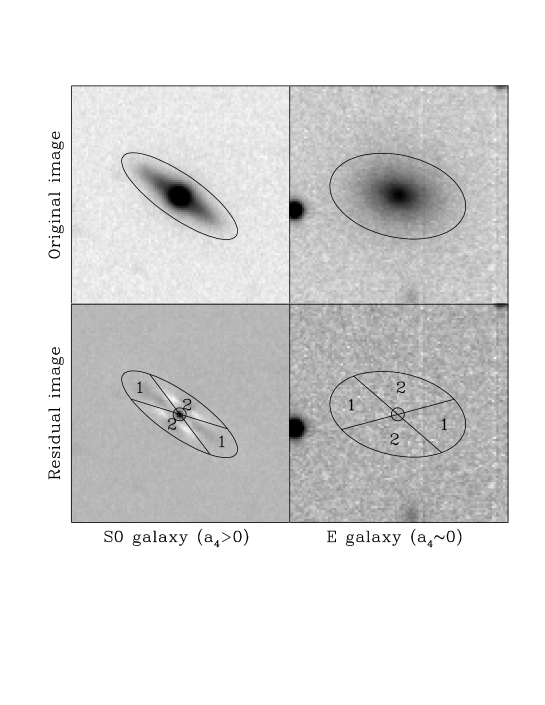
Figure 19: Illustration of the diagnostic $D_{10}$ (see text for a detailed explanation).

Figure 20: Illustration of the diagnostic $D_{11}$ (see text for a detailed explanation).

The second diagnostic ($D_{11}$) is defined as the correlation coefficient (C.C.) between the counts of the pixels within whatever half-part of the model-ellipse (for instance the bottom-half: Y${}_{pix}\leq$Y_cen) and those of the corresponding pixels symmetric with respect to the galaxy center. In Figure 20 these two quantities are plotted against each other for the same galaxies used in Figure 19, i.e. a S0 galaxy with disky isophotes (left panel) and an elliptical galaxy (right panel). It is evident that high values of C.C. correspond to strongly disk-shaped objects, while for regular (non disky) ellipticals the C.C. values are close to zero;

$D_{12}$: Bandwidth of Power Spectrum.

Roughly speaking, late–type galaxies are dominated by structural features (spiral arms, clumps, tails, blobs, etc..) whose size is (much) lower than galaxy size, while elliptical and (in general) early–type galaxies are typically dominated by a single, regular structure, whose size is comparable with that of the galaxies themselves. Having this in mind, we have devised a new morphological diagnostic defined as the ratio between some characteristic inverse frequency of the 2D power spectrum of the galaxy image (i.e. the typical size of features) and the equivalent threshold radius of the galaxy ($\sqrt{A_{thr}/\pi}$). Operatively, we estimate the characteristic size of galaxy features by processing the $F_{C}$ image with the powerspec tool (option: center=yes) included in the IRAF stsdas-Fourier package (FFT), and computing on the powerspec image the equivalent radius of the area where the power exceeds half of the maximum FFT power.

The next four morphological diagnostics concern the statistical behaviour of very local pixel properties (image texture; a similar approach can be found in Moore et al., 2006) over the whole galaxy body. In particular, they consider the texture unities ($TUs$ hereafter) provided by all the 3$\times$3 pixel squares centered on each pixel of the frame $F_{C}(i,j)$ for $i=j=$2,…,(N-1). In order to make easier the formalism related to these diagnostics, it is convinient to introduce the following definitions relative to each $TU_{ij}$ (see Figure 21):

Figure 21: Scheme of a Texture Unit (TU_ij), illustrating the meaning of its upper indices (see the formulation in the text).

$f_{ij}=F_{C}(i,j)$;

$f_{ij}^{1-}=F_{C}(i-1,j)$; $f_{ij}^{1+}=F_{C}(i+1,j)$;

$f_{ij}^{2-}=F_{C}(i-1,j-1)$; $f_{ij}^{2+}=F_{C}(i+1,j+1)$;

$f_{ij}^{3-}=F_{C}(i,j-1)$; $f_{ij}^{3+}=F_{C}(i,j+1)$;

$f_{ij}^{4-}=F_{C}(i+1,j-1)$; $f_{ij}^{4+}=F_{C}(i-1,j+1)$;

$\cos\alpha_{ij1}=|i-i_{c}|/d_{ij}$; $\cos\alpha_{ij2}=|i+j-i_{c}-j_{c}|/d_{ij}\sqrt{2}$;

$\cos\alpha_{ij3}=|j-j_{c}|/d_{ij}$; $\cos\alpha_{ij4}=|i-j|/d_{ij}\sqrt{2}$,

where $i_{c}\equiv j_{c}\equiv$(N/2+0.5) are the coordinates of the center, $d_{ij}=\sqrt{(i-i_{c})^{2}+(j-j_{c})^{2}}$ is the distance from the center of the pixel ($i,j$) and $\alpha_{ijk}$ ($k$=1,..,4) is the angle between the direction $(k-)\leftrightarrow(k+)$ in the $TU_{ij}$ of Figure 21 and the line connecting ($i,j$) with the galaxy center.

$D_{13}$: Average Concaveness.

Again roughly speaking, the earlier the morphological type, the lower the unevennes of the intensity surface of the galaxy. Moreover, while in early–type galaxies the intensity gradient increases regularly toward the center over almost the whole galaxy body, for late–type objects, due to the presence of relatively small structural features (spiral arms, clumps, tails, blobs, etc..), such regular behaviour is limited to the very inner part of the galaxy (bulge). That being stated and given the above definitions, this new diagnostic is expressed by the formula:

$$D_{13}=0.5+{\displaystyle\sum_{i,j=2}^{N-1}{f_{ij}\times sgn\big{\{}\sum_{k=1}^{4}{\cos\alpha_{ijk}(f_{ij}^{k-}+f_{ij}^{k+}-2f_{ij})\big{\}}}}\over\displaystyle{2\times\sum_{i,j=2}^{N-1}{f_{ij}}}}$$

which in fact provides the fraction of the total galaxy luminosity coming from pixels ($i,j$) for which is positive the local concaveness, computed in the corresponding $TU_{ij}$ and weight-averaged according to the direction of the galaxy center ($\cos\alpha_{ijk}$). In the above formula, $sgn$ is the sign function: $sgn(x)$=-1,0,1 for $x<$0, $x$=0 and $x>$0, respectively.

$D_{14}$: Monotonicity.

Likewise the previous diagnostic, this one too deals with some geometrical rule to which the intensities inside $TUs$ should obey. In particular, in this case we consider the fraction of the total galaxy luminosity coming from pixels ($i,j$) for which $F_{C}(i,j)$ has a monotonic behaviour in all the four directions of $TU_{ij}$ illustrated in Figure 21. Again, the greater the amount of structural features (late–type galaxies), the lower the expected fraction. In formula:

$$D_{14}=1+{\displaystyle\sum_{i,j=2}^{N-1}{f_{ij}\times sgn\big{\{}\sum_{k=1}^{4}{(\delta f_{ij}^{k\pm}-\delta f_{ij}^{k-}-\delta f_{ij}^{k+})\big{\}}}}\over\displaystyle{\sum_{i,j=2}^{N-1}{f_{ij}}}}$$

where:

$\delta f_{ij}^{k\pm}$=$|f_{ij}^{k-}-f_{ij}^{k+}|$, $\delta f_{ij}^{k+}$=$|f_{ij}^{k+}-f_{ij}|$ and $\delta f_{ij}^{k-}$=$|f_{ij}^{k-}-f_{ij}|$.

$D_{15}$: Alignment.

In defining the next two diagnostics it is convenient to convert the pixel coordinates in the reference system of the circularized ellipse, whose ellipticity and position angle ($\varepsilon,\theta$) are those previously determined (Section 3.1.1) and assumed to be the global geometrical parameters of the galaxy:

$x_{ij}=[(i-i_{c})\cos\theta+(j-j_{c})\sin\theta]\times\sqrt{1-\varepsilon}$;

$y_{ij}=[(j-j_{c})\cos\theta+(i-i_{c})\sin\theta]$/$\sqrt{1-\varepsilon}$;

$z_{ij}=F_{C}(i,j)$.

Using this system of coordinates, the new diagnostic ($D_{15}$) tries to quantify to which degree the local maximum intensity gradient is aligned with the galaxy center over the whole galaxy body. Again, the presence of small scale structures in late–type galaxies should imply a lower degree of alignment of the local maximum gradient toward the galaxy center with respect to early–type galaxies. To quantify such degree of alignment, the points in the space ($x,y,z$) corresponding to the nine pixels of each $TU_{ij}$ have been linearly interpolated ($\chi^{2}$) by the function: $Z_{ij}(x,y)=a_{ij}+b_{ij}x+c_{ij}y$. Then, for each $TU_{ij}$, we have computed the angle $\phi_{ij}$ between two planes, both passing through the point [$x_{ij},y_{ij},Z_{ij}(x_{ij},y_{ij})$] and parallel to the $z$ axis. The first plane contains the galaxy center (origin of the new coordinates system), while the second one is parallel to the line of maximum intensity gradient in the previous linear interpolation. Finally, the cosines of the angles $\phi_{ij}$ have been weight-averaged over the whole frame, according to the local intensity. In formula:

$$D_{15}={\sum_{i,j=2}^{N-1}{z_{ij}\times\cos\phi_{ij}}\over{\sum_{i,j=2}^{N-1}{z_{ij}}}}$$

where the cosines:

$$\cos\phi_{ij}={{b_{ij}x_{ij}+c_{ij}y_{ij}}\over{\sqrt{(x_{ij}^{2}+y_{ij}^{2})(b_{ij}^{2}+c_{ij}^{2})}}}$$

turn out to be positive if the function $Z_{ij}(x,y)$ increases toward the galaxy center at the point ($i,j$), while they are negative in the opposite case.

$D_{16}$: Intercept Angle.

In defining the previous diagnostic we have introduced the local planes $Z_{ij}(x,y)$ interpolating the nine points ($x,y,z$) of each $TU_{ij}$. We noted that in early–type galaxies the line of maximum gradient of these planes should be (on average) more oriented towards the center than in the case of late–type galaxies and that such alignment should be more and more pronounced at increasing the intensity and decreasing the distance from the galaxy center. Here we note that, in addition, the average values of the intercept ($a_{ij}$) between these planes and the $z$ axis should be higher in early–type than in late–type galaxies, where the irregular intensity surface should make almost randomly distributed both the orientations and the intercept levels of the planes, especially in the intermediate and outer regions of galaxies. In order to quantify such average intercept level avoiding computational divergences, we actually prefer to deal with the cosines of the angles ($\beta_{ij}$) between the $z$ axis and the stright lines connecting the points ($x_{ij},y_{ij},0$) and ($a_{ij},0,0$). Since the values of $\cos\beta_{ij}$ obviously depend on the units used to measure intensities and radii, it is necessary to normalize both quantities. We decided to normalize the intensities at $z_{c}=F_{C}(i_{c},j_{c})$ (intensity of the galaxy center) and the radii at: $R_{thr}=\sqrt{A_{thr}/\pi}$ (equivalent radius of the threshold area). After some algebra, the new diagnostic, that is the normalized, average $\cos\beta$ is defined as follows:

$$D_{16}={\sum_{i,j=2}^{N-1}{W_{ij}\times a_{ij}/\sqrt{a_{ij}^{2}+d_{ij}^{2}K^{2}}}\over{\sum_{i,j=2}^{N-1}{W_{ij}}}}$$

where: $d_{ij}=\sqrt{x_{ij}^{2}+y_{ij}^{2}}$ is the circularized distance from the galaxy center, $K=z_{c}/R_{thr}$ is the normalization factor and $W_{ij}=z_{ij}/d_{ij}$ are the weighting factors, which increase at increasing the local intensity and at decreasing the distance from the galaxy center.

$D_{17}-D_{20}$: Intensity distribution moments.

The last four diagnostics simply concern the moments of the intensity distribution within the galaxy frame. In particular, we consider the median ($D_{17}$), the standard deviation ($D_{18}$), the skewness ($D_{19}$) and the kurtosis ($D_{20}$) of the distribution of the pixel intensities, normalized to their average value.

Appendix B The Maximum Likelihood technique

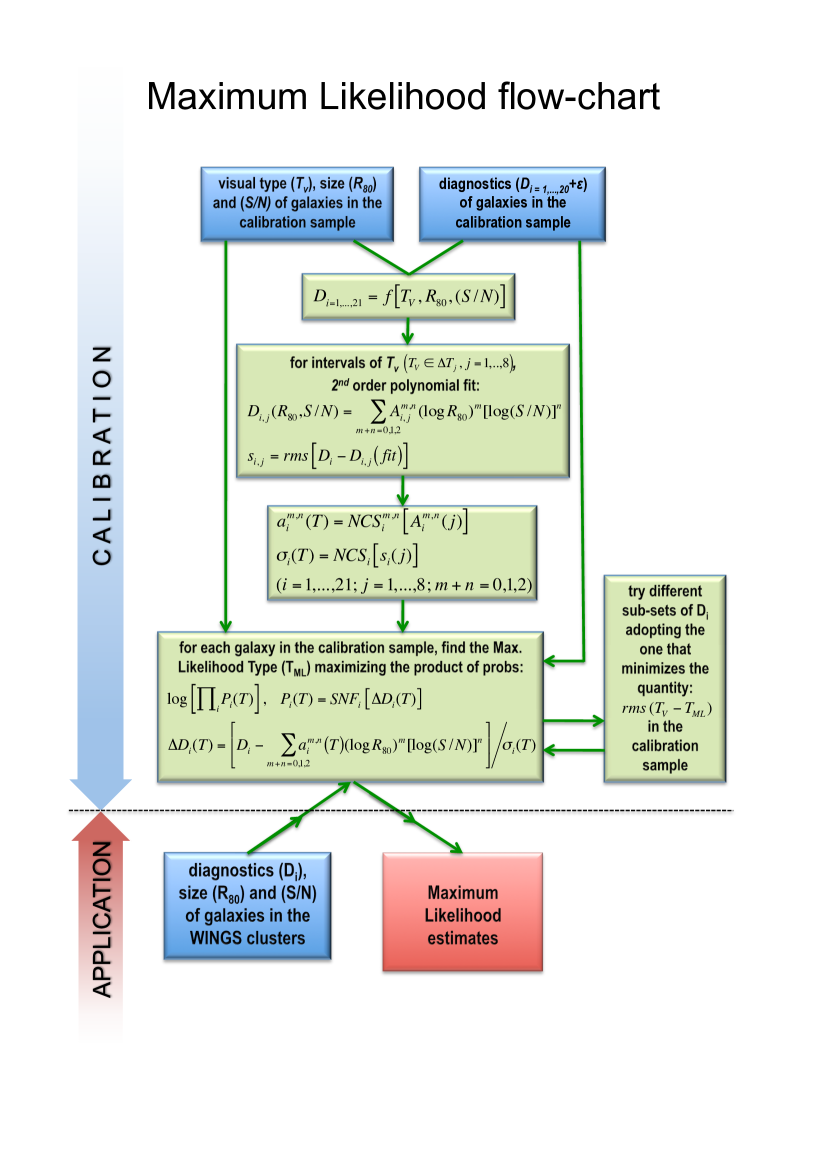
Figure 22: Flow-chart of the MORPHOT Maximum Likelihood tool

The flow-chart in Figure 22 should help the reader in this section, leading her/him through the various steps of this semi-analytical technique. As already mentioned in Section 3.2.1, besided obviously depending on the visual morphological type (Figure 5), the diagnostics $D_{i}$ turn out to depend on both the seeing normalized size [$\log(R_{80}/FWHM)$] and the signal-to-noise ratio [$\log(S/N)$] (Figure 7). Therefore, prior to use them to gauge the morphology of galaxies, we have to remove these two dependences, thus picking out the net dependence of each diagnostic on the morphological type.

To this aim the whole range of morphological types in the calibration sample has been divided into eight, nearly omogeneous intervals (see the plots on the right side of Figure 23). For each interval $\Delta T_{j}$ (j=1,…,8), the dependences of all the diagnostics $D_{i}$ (i=1,…,21) on $R_{80}$ and $S/N$, have been represented (through least square fitting) by the following second order polynomial functions:

$$D_{i,j}(R_{80},S/N)=\displaystyle\sum_{m+n=0,1,2}{A_{ij}^{m,n}\log(R_{80}/FWHM)^{n}\log(S/N)^{m}}$$

thus producing, for each $D_{i}$ and for each $\Delta T_{j}$, the coefficients $A_{ij}^{m,n}$ and the $rms$ scatters $s_{i,j}$ of the residuals with respect to the fits. Then, for each $D_{i}$, these quantities have been interpolated, as a function of the morphological type, with Natural Cubic Splines ($NCS$):

$$a_{i}^{m,n}(T)=NCS_{i}^{m,n}[A_{i}^{m,n}(j)];\hskip 8.5359pt\sigma_{i}(T)=NCS_{i}[s_{i}(j)]$$

An example of this procedure is shown in the plots on the left side of Figure 23, which is referred to the diagnostic $D_{13}$, defined in Appendix A. Because of the evident discontinuity between cD and E galaxies, the first bin ($\Delta T_{1}$) has been excluded from the spline fitting. Such discontinuity is actually found also for the coefficients $A^{m,n}$ of the other diagnostics and reflects their peculiar behaviour for $T_{M}$=$-6$ (see Figure 5). It is likely telling us once again that cD galaxies are quite apart from Es and, in general, from all ’normal’ galaxies, thus suggesting they are the product of a peculiar evolutionary path (Fasano et al., 2010). The right side of Figure 23 shows (again in the case of $D_{13}$) the residuals of the above mentioned polynomial fits with respect to both $\log(R_{80}/FWHM)$ (upper panels inside each $\Delta T_{j}$ heavy box) and $\log(S/N)$ (lower panels in the same boxes).

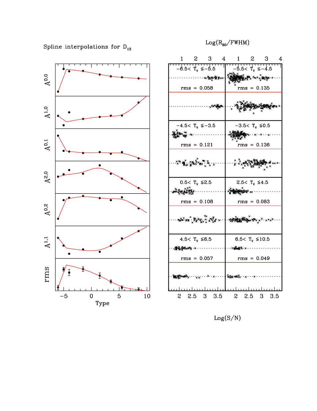
Figure 23: Example of the fitting procedure performed in order to remove the dependence of morphological diagnostics on the size ($R_{80}$) and signal to noise ratio ($S/N$). The case of the diagnostic $D_{13}$ is illustrated in the figure. Left panels: Natural Cubic Spline (NCS) fitting of the polynomial coefficients $A_{13}^{m,n}$ and of the scatter $\sigma_{13}$ as a functions of the morphological type (details in the text). Right panels: Residuals of the (polynomial+spline) fits illustrated in the left panels with respect to both $\log(R_{80}/FWHM)$ and $\log(S/N)$. In particular, the upper panels inside each $\Delta T_{j}$ tick line box show the residuals as a function of $\log(R_{80}/FWHM)$ (units at the top of the figure), while the lower panels in each tick line box show the corresponding residuals as a function of $\log(S/N)$ (units at the bottom of the figure).

The previous formulae allow us to remove the dependence of diagnostics on $R_{80}$ and $S/N$. Consider now a galaxy for which we know the diagnostics $D_{i}$ and the quantities $R_{80}/FWHM$ and $S/N$. For any given morphological type $T$ and for each diagnostic, the deviations of the actual values of $D_{i}$ with respect to those obtained from the above fitting procedure, normalized by the corresponding expected scatter, can be expressed as follows:

$$\Delta D_{i}(T)={{D_{i}-\displaystyle\sum_{m+n=0,1,2}a_{i}^{m,n}(T)\log(R_{80}/FWHM)^{n}\log(S/N)^{m}}\over{\sigma_{i}(T)}}$$

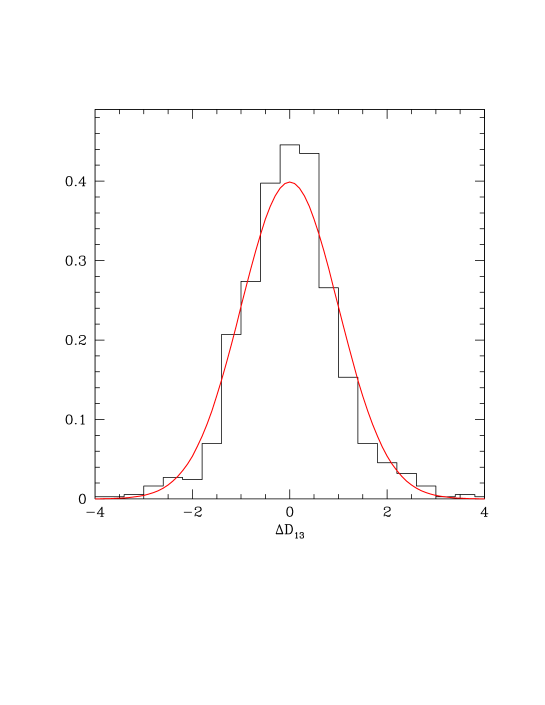
Figure 24: Distribution of the deviates of the morphological diagnostics of the calibration galaxy sample with respect to the polynomial+spline fitting (details in the text) performed in order to remove their dependence on the size ($R_{80}$) and signal to noise ratio ($S/N$).

If we assume the distributions of the deviates to be normal (a fair assumption, in our case; see Figure 24), the probability that the actual value of the diagnostic $D_{i}$ is found for a galaxy of morphological type $T$, can be expressed by:

$$P_{i}(T)=SNF_{i}[\Delta D_{i}(T)]$$

($SNF[x]$=$e^{-x^{2}/2}/\sqrt{2\pi}$ is the Standardized Normal Function) and the Maximum Likelihood (ML) probability that the morphological type $T$ is associated to the actual set of diagnostics $D_{i}$ ($i$=1,…,21) can be obtained through the product of the individual probabilities:

$$P(T)=\prod_{i=1,21}P_{i}(T)$$

We actually prefer to use the logarithmic form:

$$\log[P(T)]=\displaystyle\sum_{i=1,21}w_{i}\times\log[P_{i}(T)]$$

where $w_{i}$ are binary weighting factors (0/1) which determine the inclusion of each diagnostic in the final adopted set of $D_{i}$ (see Section 3.3.1 and Figure 8).

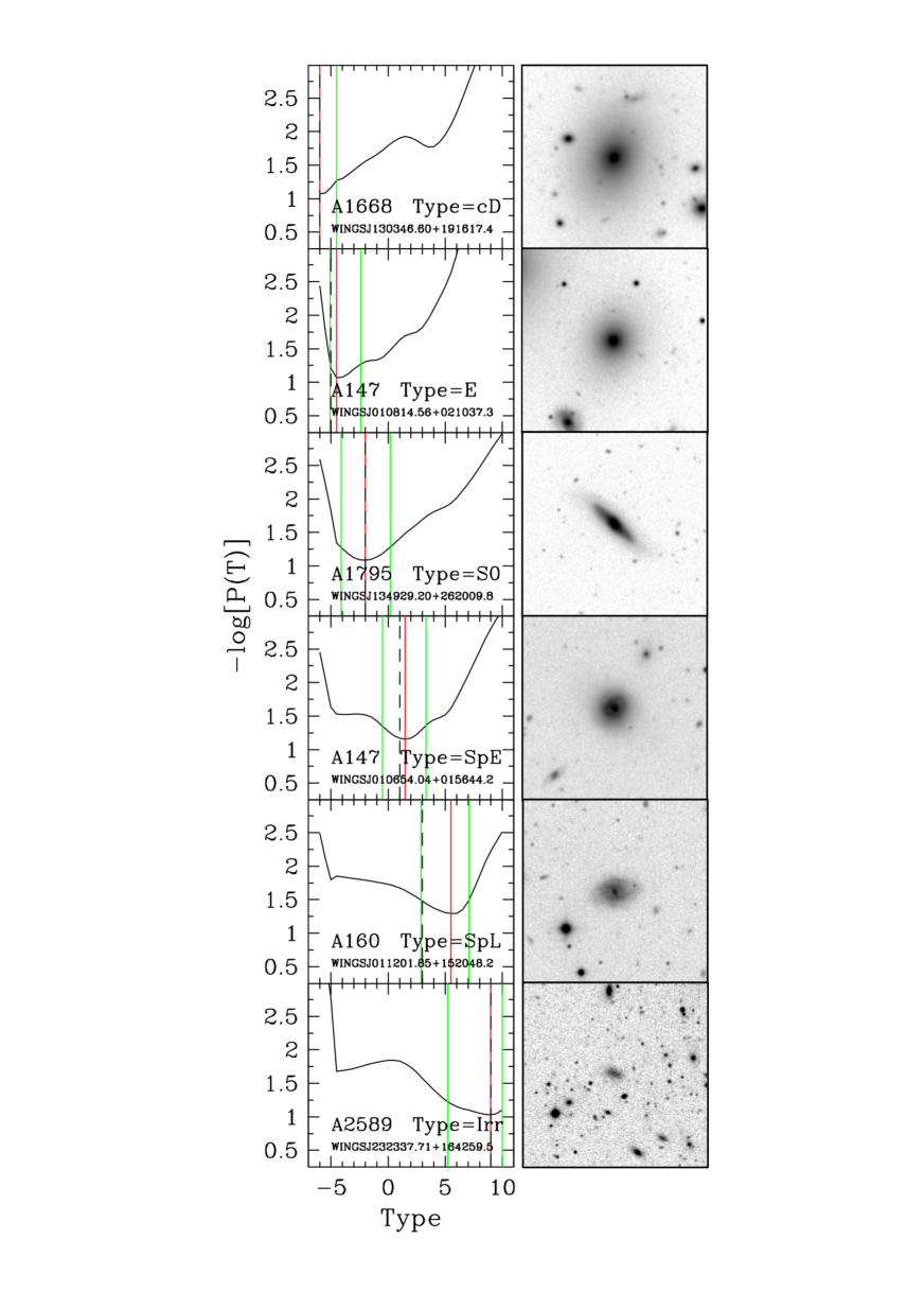
Figure 25: Examples of the Maximum Likelihood minimization for WINGS galaxies of different ’broad’ morphological classes.

We compute the above probability from $T$=$-6.5$ to $T$=10.5 (step 0.1) and we assume the ML morphological estimator to be the value of $T$ which minimizes the $-\log[P(T)]$. Figure 25 shows some examples of the behaviour of the ML probability as a function of the morphological type for typical galaxies belonging to the six above defined broad morphological classes. The red lines in each left side figure mark the minimum values of $-\log[P(T)]$, i.e. the adopted MORPHOT-ML morphological types $T_{ML}$, while the dashed lines indicate the corresponding visual estimates $T_{V}$. Conventionally, we should obtain the confidence intervals of our ML estimates by the change in $T$ necessary to decrease $P(T)$ by $\Delta P$=0.5 from its value at the maximum (in logarithm: $\Delta\log P\sim$0.3). In practics, numerical simulations of the MORPHOT-ML technique and visual inspection of several real cases suggest that a value of $\Delta\log P\sim$0.2 provides more realistic boundaries to the morphological estimates. The green lines in Figure 25 set the confidence intervals obtained in this way. Note in the figure the discontinuity between cD and E galaxies already shown in Figure 23 and commented before. Note also the discrepancy between visual and ML estimates in the case of the galaxy in Abell 160, which has been visually classified early-spiral and automatically classified late-spiral ($\Delta T\sim$2.5).

Appendix C The Neural Network technique

The architecture and strategy adopted to produce a Neural Network estimator for the morphological classification are very similar to that described in Vanzella et al. (2004). Here be briefly recall the method.

C.0.1 Architecture

We adopt the classical feed-forward multilayer perceptron Neural Network (MLP, Bishop 1995) with four layers, each one made of 23, 20, 20 and 1 nodes. The first layer (named input layer) receives 23 input parameters for each galaxy (i.e. the diagnostics $D_{i}$, $i$=1,…,20 as described in Appendix A and the global quantities $\varepsilon$, $\log[R_{80}/FWHM]$ and $\log[S/N]$), while the single output node (output layer) produces the morphological evaluation. The other two layers of 20 nodes each are called hidden layers. Each node of a layer is connected to all the nodes of the next layer.

C.0.2 Training

We use the supervised learning method, i.e. the NN is trained with examples. The training set is composed by the 926 galaxies in the calibration sample, each one visually classified ($T_{V}$). Each example presented to the NN is a pair of arrays, one contains the set of diagnostics (described in Appendix A) with 23 components and the second array is the targeted morphology (single component), $T_{V}$. The learning algorithm modifies the strength of the connections between nodes (called weights) in order to force the association between the input and the correct output. It translates to a minimization of a merit function as a function of the set of weights.

Once a suitable set of weights is determined, it is frozen and stored for evaluation of new (never seen) galaxies. There are various techniques to identify the best set of weights, i.e. those that offer the so called best generalization power and that avoid the over-fitting problem. Here we adopt the method based on a committee of neural networks (30 MLPs have been used) as described in Vanzella et al. (2004). This method reduce the variance in the predictions maintaining a relatively small bias (Bishop, 1995). Each member of the committee has been trained with different initial conditions (e.g. initial random distribution of weights, random sequence of examples presented to the NN, bootstrapping of examples), that produce different histories of training and 30 different set of weights. Therefore, for each galaxy, the committee produces 30 estimations of the morphology ($T_{NN}^{i}$, $i$=1-30). From this distribution we extract the median(mean) $T_{NN}$ of the $T_{NN}^{i}$ and the central 68% interval (16 and 84 percentiles). With this method we can associate a statistical uncertainty to the predicted value $T_{NN}$.

It is clear that the outlined weighting of the connections, inherent to this methodology, automatically provides the selection of the most significant diagnostics, thus making useless the preliminar (empirical) choice we performed in the case of the ML technique.

References

- Abraham et al. (1996) Abraham, R.G., Tanvir, N.R., Santiago, B.X., Ellis, R.S., Glazebrook, K., & van den Bergh, S. 1996, MNRAS, 279, L47
- Abraham et al. (2003) Abraham, R. G., van den Bergh, S., & Nair, P. 2003, ApJ, 588, 218
- Ball et al. (2004) Ball, N.M., Loveday, J., Fukugita, M., Nakamura, O., et al. 2004, MNRAS, 348, 1038
- Bell et al. (2004) Bell, E. F., et al. 2004, ApJLett., 600, 11
- Bender and Moellenhoff (1987) Bender, R., & Moellenhoff, C. 1987, A&A, 177, 71
- van den Bergh (1959) van den Bergh, S. 1959, AJ, 64, 347
- van den Bergh (1960a) van den Bergh, S. 1960, ApJ, 131, 215
- van den Bergh (1960b) van den Bergh, S. 1960, ApJ, 131, 558
- Bertin and Arnouts (1996) Bertin, E., & Arnouts, S. 1996, A&A, 117, 393
- Bishop (1995) Bishop, C. M. 1995, Neural networks for pattern recognition (Oxford University Press)
- Buta (2011) Buta, R.J. 2011, arXiv:astro-ph/1102.0550
- Calvi et al. (2011) Calvi, R., Poggianti, B.M., & Vulcani, B. 2011, arXiv:astro-ph/1105.3683
- Capaccioli et al. (1991) Capaccioli, M., Vietri, M., Held, E.V., & Lorenz, H. 1991, ApJ, 371, 535
- Cappellari et al. (2011) Cappellari, M., etal. 2011, arXiv:1104.3545
- Cassata et al. (2010) Cassata, P., Giavalisco, M., Guo, Yicheng, Ferguson, H., Koekemoer, A. M., Renzini, A., Fontana, A., Salimbeni, S., Dickinson, M., Casertano, S., et al. 2010, ApJ, 714, L79
- Cava et al. (2009) Cava, A., et al. 2009, A&A, 495, 707
- Cheng et al. (2011) Cheng, J.Y., Faber, S.M., Simard, L., Graves, G.J., et al. 2011, MNRAS, 412, 727
- Conselice (1997) Conselice, C. J. 1997, PASP, 109, 1251
- Conselice et al. (2000) Conselice, C. J., Bershady, M.A., & Jangren, A. 2000, ApJ, 529, 886
- Conselice (2003) Conselice, C. J., 2003, ApJS, 147, 1
- Couch et al. (1994) Couch, W. J., Ellis, R. S., Sharples, R. M., & Smail, I. 1994, ApJ, 430, 121
- Couch et al. (1998) Couch, W. J., Barger, A. J., Smail, I., Ellis, R. S., & Sharples, R. M. 1998, ApJ, 497, 188
- de la Calleja and Fuentes (2004) de la Calleja, J., & Fuentes, O. 2004, MNRAS, 349, 87
- Desai et al. (2007) Desai, V., et al. 2007, ApJ, 660, 1151
- D’Onofrio et al. (2011) D’Onofrio et al. 2011, ApJ, in preparation
- Dressler et al. (1997) Dressler, A., Oemler, A., Jr., Couch, W. J., Smail, I., Ellis, R. S., Barger, A., Butcher, H., Poggianti, B. M., & Sharples, R. M. 1997, ApJ, 490, 577
- Ebeling et al. (1996) Ebeling, H., Voges, W., Bohringer, H., Edge, A. C., Huchra, J. P., & Briel, U. G. 1996, MNRAS, 281, 799
- Ebeling et al. (1998) Ebeling, H., Edge, A. C., Bohringer, H., Allen, S. W., Crawford, C. S., Fabian, A. C., Voges, W., & Huchra, J. P. 1998, MNRAS, 301, 881
- Ebeling et al. (2000) Ebeling, H., Edge, A. C., Allen, S. W., Crawford, C. S., Fabian, A. C., & Huchra, J. P. 2000, MNRAS, 318, 333
- Elmegreen et al. (1987) Elmegreen, D. M., Elmegreen, B. G. 1987, ApJ, 314, 3
- Fasano et al. (1991) Fasano, G., & Vio, R. 1991, MNRAS, 249, 629
- Fasano et al. (1993) Fasano, G., Amico, P., Bertola, F., Vio, R. & Zeilinger, W.W. 1993, MNRAS, 262, 109
- Fasano et al. (2000) Fasano, G., Poggianti, B. M., Couch, W. J., Bettoni, D., Kjærgaard, P., & Moles, M. 2000, ApJ, 542, 673
- Fasano et al. (2006) Fasano, G., Marmo, C., Varela, J., D’Onofrio, M., Poggianti, B.M., Moles, M., Pignatelli, E., Bettoni, D., et al. 2006, A&A, 445, 805
- Fasano et al. (2007) Fasano, G., et al. 2007, From Stars to Galaxies: Building the Pieces to Build Up the Universe, A. Vallenari, R. Tantalo, L. Portinari, & A. Moretti, ASP Conference Series, 374, 495
- Fasano et al. (2010) Fasano, G., Bettoni, D., Ascaso, B., Tormen, G., Poggianti, B.M., Valentinuzzi, T., D’Onofrio, M., et al. 2010, MNRAS, 404, 1490
- Fritz et al. (2007) Fritz, J., Poggianti, B.M., Bettoni, D., Cava, A., Couch, W.J., D’Onofrio,M., Dressler, A., Fasano, G., et al. 2007, A&A, 470, 137
- Fritz et al. (2011) Fritz, J., Poggianti, B.M., Cava, A., Valentinuzzi, T., Moretti, A., Bettoni, D., Bressan, A., Couch, W.J., et al. 2011, A&A, 526, 45
- Fukugita et al. (2007) Fukugita, M., Nakamura, O., Okamura, S., Yasuda, N., et al. 2007, AJ, 134, 579
- Goderya et al. (2004) Goderya, S., Andreasen, J. D., & Philip, N. S. 2004, ASP Conference Proceedings, 314, 617
- Graham et al. (2001) Graham, A. W., Trujillo, I., & Caon, N. 2001, AJ, 122, 1707
- Gutierrez et al. (2004) Gutierrez, C. M., Trujillo, I., Aguerri, J. A. L., Graham, A. W., & Caon, N. 2004, ApJ, 602, 664
- Hansson et al. (2011) Hansson, K.S.A., Poggianti, B.M., Feltzing, S., Cava, A., Fritz, J., Fasano, G., et al. 2011, A&A, submitted
- Hatziminaoglou et al. (2005) Hatziminaoglou, E., et al. 2005, MNRAS, 364, 47
- Holmberg (1950) Holmberg, E. 1950, Lund Medd. Astron. Obs. Ser. II, 128, 1
- Hubble (1922) Hubble, E. P. 1922, ApJ, 56, 162
- Hubble (1925) Hubble, E. P. 1925, ApJ, 62, 409
- Hubble (1926) Hubble, E. P. 1926, ApJ, 64, 321
- Hubble (1936) Hubble, E. P. 1936, Realm of the Nebulae, New Haven: Yale University Press
- Huertas-Company et al. (2008) Huertas-Company, M., Rouan, D., Tasca, L., Soucail, G., & Le Fèvre, O. 2008, A&A, 478, 971
- Kelly and McKay (2004) Kelly, B. C., & McKay, T. A. 2004, AJ, 127, 625
- Kelson et al. (1997) Kelson, D. D., van Dokkum, P. G., Franx, M., Illingworth, G. D., & Fabricant, D. 1997, ApJLett., 478, 13
- La Barbera et al. (2008) La Barbera, F., de Carvalho, R. R., Kohl-Moreira, J. L., Gal, R. R., Soares-Santos, M., Capaccioli, M., Santos, R., & Sant’anna, N. 2008, PASP, 120, 681
- Lauger et al. (2005) Lauger, S., Burgarella, D., & Buat, V. 2005, A&A, 434, L77
- Lintott et al. (2011) Lintott, C., Schawinski, K., Bamford, S., et al. 2011, MNRAS, 410, 166
- Lotz et al. (2004) Lotz, J. M., Primack, J., & Madau, P. 2004, AJ, 128, 163
- Lubin et al. (1998) Lubin, L. M., Postman, M., Oke, J. B., Ratnatunga, K. U., Gunn, J. E., Hoessel, J. G., & Schneider, D. P. 1998, ApJLett., 478, 13
- Menanteau (2006) Menanteau, F. 2006, Bulletin of the American Astronomical Society, 38, 134
- Méndez-Abreu et al. (2008) Méndez-Abreu, J., Aguerri, J. A. L., Corsini, E. M. & Simonneau, E. 2008, A&A, 478, 353
- Moore et al. (2006) Moore, J.A., Pimbblet, K.A., & Drinkwater, M.J. 2006, PASA, 23, 135
- Morgan (1958) Morgan, W. W. 1958, PASP, 70, 364
- Naim et al. (1995) Naim, A., Lahav, O., Sodré, L. & Storrie-Lombardi, M.C., 1995, MNRAS, 275, 567
- Naim et al. (1997) Naim, A., Ratnatunga, K.U., & Griffiths, R.E., 1997, ApJS, 111, 357
- Nair et al. (2010) Nair, P.B., & Abraham, R.G., 2010, ApJS, 186, 427
- Oemler et al. (1997) Oemler, A., Jr., Dressler, A., & Butcher, H. R. 1997, ApJ, 474, 561
- Odewahn et al. (2002) Odewahn, S. C., Cohen, S. H., Windhorst, R. A., & Philip, N. S. 2002, ApJ, 568, 539
- Omizzolo et al. (2011) Omizzolo, A., et al. 2011, in preparation
- Örndahl and Rönnback (2005) Örndahl, E. & Rönnback, J. 2005, A&A, 443, 61
- Pascarelle et al. (1995) Pascarelle, S. M., Windhorst, R. A., Odewahn, S. C., & Keel, W. C. 1995, Bulletin of the American Astronomical Society, 27, 1442
- Peng et al. (2002) Peng, C. Y., Ho, L. C., Impey, C. D., & Rix, H. W. 2002, AJ, 124, 266
- Petty (2009) Bulletin of the American Astronomical Society, 41, 512
- Pignatelli et al. (2006) Pignatelli, E., Fasano, G., & Cassata, P. 2006, A&A, 446, 373
- Poggianti et al. (2009) Poggianti, B. M., et al. 2009, ApJLett., 697, 137
- Postman et al. (2005) Postman, M., et al. 2005, ApJ, 623, 721
- Rahman and Shandarin (2004) Rahman, N., & Shandarin, S.F. 2004, MNRAS, 354, 235
- Raynolds (1920) Raynolds, J.H. 1920, MNRAS, 80, 746
- Ravindranath et al. (2006) Ravindranath, S., et al. 2009, ApJ., 652, 963
- Richter et al. (1991) Richter, G. M., Bohm, P., Lorenz, H., & Priebe, A. 1991, Astron.Nachr., 312, 346
- Saintonge et al. (2005) Saintonge, A., Schade, D., Ellingson, E., Yee, H. K. C., & Carlberg, R. G. 2005, ApJS, 157, 228
- Sánchez-Janssen et al. (2011) Sánchez-Janssen, R., Aguerri, A., et al. 2011, in preparation
- Sánchez-Portal et al. (2004) Sánchez-Portal, M., Diaz, A. I., Terlevich, E., Terlevich, R. 2004, MNRAS, 350, 1087
- Scarlata et al. (2007) Scarlata, C., et al. 2007, ApJS, 172, 406
- Shamir (2009) Shamir, L. 2009, MNRAS, 399, 1367
- Shamir (2011) Shamir, L. 2011, arXiv:astro-ph/1105.3214
- Simard (1998) Simard, L. 1998, A.S.P. Conference Series, 145, 108
- Smail et al. (1997) Smail, I., Dressler, A., Couch, W. J., Ellis, R. S., Oemler, A., Jr., Butcher, H., & Sharples, R. M. 1997, ApJ, 110, 213
- Tasca and White (2005) Tasca, L. A. M., & White, S. D. M. 2005, arXiv:astro-ph/0507249
- Treu et al. (2003) Treu, T., Ellis, R. S., Kneib, J. P. Dressler, A. Smail, I., Czoske, O., Oemler, A., & Natarajan, P. 2003, ApJ, ,
- Trujillo et al. (2001) Trujillo, I., Aguerri, J. A. L., Cepa, J. & Gutierrez, C. M. 2001, MNRAS, 321, 269
- Trujillo and Aguerri (2004) Trujillo, I., & Aguerri, J. A. L. 2004, MNRAS, 355, 82
- Valentinuzzi et al. (2009) Valentinuzzi, T., Woods, D., Fasano, G., Riello, M., D’Onofrio, M., Varela, J., Bettoni, D., Cava, A., et al. 2009, A&A, 501, 851
- Vanzella et al. (2004) Vanzella, E., et al. 2004, A&A, 423, 761
- van der Wel (2008) van der Wel, A. 2008, ApJ, 675, 13
- Varela et al. (2009) Varela, J., et al. 2009, A&A, 497, 667
- Vulcani et al. (2011) Vulcani, B., Poggianti, B.M., Dressler, A., Fasano, G., Valentinuzzi, T., Couch, W., Moretti, A., et al. 2011, MNRAS, 413, 921
- de Vaucouleurs (1959) de Vaucouleurs, G. 1959, ApJ, 130, 718
- de Vaucouleurs (1963) de Vaucouleurs, G. 1963, ApJS, 8, 31
- de Vaucouleurs (1974) de Vaucouleurs, G. 1974, The formation and dynamics of galaxies, IAU Symp., 58, 1
- de Vaucouleurs et al. (1991) de Vaucouleurs, G., de Vaucouleurs, A., Corwin, H. G., Jr., Buta, R. J., Paturel, G., & Fouqué, P. 1991, Third Reference Catalogue of Bright Galaxies, Springer, New York, NY (USA)
- Vikram et al. (2010) Vokram, V., Wadadekar, Y., Kembhavi, A.K., & Vijayagovindan, G.V. 2010, MNRAS, 409, 1379
- Yamauchi et al. (2005) Yamauchi, C., Ichikawa, S., Doi, M., Yasuda, N., Yagi, M., Fukugita, M., Okamura, S., Nakamura, O., Sekiguchi, M., & Goto, T. 2005, AJ, 130, 1545
- Yoon et al. (2009) Yoon, I., Weinberg, M. D., & Katz, N. S. 2009, arXiv0902.0816Y