Microscopically derived Ginzburg-Landau theory for magnetic order in the iron pnictides

Abstract

We examine the competition of the observed stripe spin density wave (SDW) with other commensurate and incommensurate SDW phases in a two-band model of the pnictides. Starting from this microscopic model, we rigorously derive an expansion of the free energy in terms of the different order parameters at the mean-field level. We show that three distinct commensurate SDW states are possible and study their appearance as a function of the doping and the electronic structure. We show that the stripe phase is generally present, but its extent in the phase diagram depends strongly upon the number of hole Fermi pockets that are nested with the electron Fermi pockets. Electron pockets competing for the same portion of a hole pocket play a crucial role. We discuss the relevance of our results for the antiferromagnetism of the pnictides.

I Introduction

The superconductivity of the iron pnictides continues to fascinate the condensed matter community.Paglione2010 ; Johnston2010 ; Lumsden2010 Because of their high critical temperatures, particular interest has focused upon the so-called 1111 familyKamihara2008 RFeAsO and the 122 familyRotter2008 $A{\rm Fe_{2}As_{2}}$ (R and A are rare-earth and alkaline-earth elements, respectively), which become superconducting by chemical doping or under pressure. The parent compounds are antiferromagnets, Lumsden2010 ; Johnston2010 with stripe-like magnetic order with respect to the lattice of Fe atoms. Furthermore, the antiferromagnetism is intimately linked to an orthorhombic distortion of the crystal, 1111coupling ; 122coupling as evidenced by the coincidence of the ferromagnetic direction with the shorter crystallographic axis in all 1111 and 122 parent compounds. It has been argued that the same condition that favors stable stripe order also implies a nematic transition above the Néel temperature $T_{N}$, where the magnetic fluctuations on each sublattice become locked into a stripe configuration,Fang2008 ; Kim2011 ; Fernandes2010 and which produces the orthorhombic distortion via the magnetoelastic coupling. Kim2011 ; BG2009 ; magph The mechanism for stabilizing the stripe order is therefore a key problem in pnictide physics.

The microscopic origin of the antiferromagnetism in the pnictides has been approached in a number of different ways. Frustrated local moment models for the Fe spins can reproduce the observed magnetic order, Johnston2010 ; localspin ; localspinorb but the evidence for the metalicity McGuire ; Liu2008 ; Dong2008 and relatively weak correlations WLYang2009 of the parent compounds, and the development of incommensurate (IC) magnetic order upon doping, Pratt2011 suggest an itinerant description. Ab initio calculations predict, nesting ; Zhang2010 and angle-resolved photoemission and magneto-oscillation experiments confirm, magneto ; ARPES that the Fermi surface of the pnictide parent compounds have quasi-two-dimensional nested electron and hole pockets. Such a system is known to undergo an excitonic instability towards a spin-density-wave (SDW) state, Excitonic ; Buker1981 as for example in chromium. Rice1970 ; Fawcett1988 Many authors have in addition emphasized the importance of the complicated orbital structure of the Fermi surfaces, Kuroki2008 ; Graser2009 ; Raghu2008 ; Nicholson2011 ; Lorenzana2008 ; Raghuvanishi2011 ; KEM2011 ; Brydon2011 ; Schmiedt2011 but key aspects of the physics are nevertheless well understood on the basis of simpler orbitally trivial “excitonic” models. Brydon2009b ; KECM2010 ; EC2010 ; KEM2011 ; FS2010 ; VVC ; ZTB2011 ; Chubukov2008 ; CT2009 ; Brydon2009a ; QI ; KESM2011 ; KT2011 ; PHW2009 ; MC2010

Most itinerant models of the pnictides display at least two nesting instabilities at different wavevectors. There is hence competition between the stripe magnetic order and other SDW phases. Within a minimal two-orbital model, Raghu2008 it has been shown that doping away from half-filling Lorenzana2008 ; Raghuvanishi2011 or a relatively large ratio of the Hund’s rule coupling to the Coulomb repulsion Raghuvanishi2011 can stabilize the stripe state. For excitonic models, on the other hand, Eremin and Chubukov EC2010 have demonstrated that the ellipticity of the electron pockets or interactions between the electron bands can stabilize the observed SDW state. The stripe order was nevertheless found to be rather sensitive to the number of Fermi pockets involved in the SDW, and its extent in the phase diagram remains uncertain. Competition with a different excitonic instability has also been proposed to stabilize a stripe SDW. KT2011

In this paper we present a systematic study of the magnetic order in the popular two-band excitonic model of the pnictides. Brydon2009b ; KEM2011 ; Nicholson2011 ; KESM2011 ; FS2010 ; VVC Keeping only interaction terms which lead to an excitonic state, we construct the Dyson equation for the single-particle Green’s functions in an arbitrary commensurate SDW phase treated at the mean-field level. By iterating the Dyson equation, we obtain approximate forms for the self-consistency equations for the order parameters valid near $T_{N}$, which we then integrate to obtain a Ginzburg-Landau expansion of the free energy. From this we determine the phase diagram for several choices of the non-interacting band structure, and show that three different commensurate SDW states are possible. We conclude with a discussion of the relevance to the magnetism of the pnictide parent compounds.

II Model

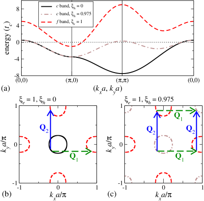
Figure 1: (color online) (a) Dispersion of the electron and hole bands for the cases of a single hole pocket at the $\Gamma$ point ($\xi_{h}=0$) and of hole pockets at both the $\Gamma$ and M points ($\xi_{h}=0.975$). Panels (b) and (c) show the corresponding Fermi surfaces and the nesting vectors ${\bf Q}_{1}=(\pi/a,0)$ and ${\bf Q}_{2}=(0,\pi/a)$. In all panels we set $\mu=0$.

We model the FeAs planes as a two-dimensional interacting two-band system, where one band has electron-like Fermi pockets, while the other has hole-like Fermi pockets. Including only interaction terms which directly lead to an excitonic instability, we write the Hamiltonian as

$$H = \sum_{{\bf{k}},\sigma}\left\{(\epsilon^{c}_{{\bf{k}}}-\mu)c^{\dagger}_{{\bf{k}}\sigma}c_{{\bf{k}}\sigma}+(\epsilon^{f}_{{\bf{k}}}-\mu)f^{\dagger}_{{\bf{k}}\sigma}f_{{\bf{k}}\sigma}\right\}$$ (1)

$${}+\frac{g_{1}}{V}\sum_{{\bf{k}},{\bf{k}}^{\prime},{\bf{q}}}\sum_{\sigma,\sigma^{\prime}}c^{\dagger}_{{\bf{k}}+{\bf{q}},\sigma}c_{{\bf{k}}\sigma}f^{\dagger}_{{\bf{k}}^{\prime}-{\bf{q}},\sigma^{\prime}}f_{{\bf{k}}^{\prime}\sigma^{\prime}}$$

$${}+\frac{g_{2}}{V}\sum_{{\bf{k}},{\bf{k}}^{\prime},{\bf{q}}}\left\{c^{\dagger}_{{\bf{k}}+{\bf{q}},\uparrow}c^{\dagger}_{{\bf{k}}^{\prime}-{\bf{q}},\downarrow}f_{{\bf{k}}^{\prime},\downarrow}f_{{\bf{k}},\uparrow}+\mbox{H.c.}\right\}\,,$$

where $c^{\dagger}_{{\bf{k}}\sigma}$ ($f^{\dagger}_{{\bf{k}}\sigma}$) creates a spin-$\sigma$ electron with momentum ${\bf{k}}$ in the hole-like (electron-like) band. In terms of the single-Fe unit cell, we assume the dispersions $\epsilon^{c}_{{\bf{k}}}=\epsilon_{c}+2t_{c}(1-\xi_{h})[\cos(k_{x}a)+\cos(k_{y}a)]+2t_{c}\xi_{h}[1+\cos(k_{x}a)\cos(k_{y}a)]$ and $\epsilon^{f}_{{\bf{k}}}=\epsilon_{f}+t_{f,1}\cos(k_{x}a)\cos(k_{y}a)-t_{f,2}\xi_{e}[\cos(k_{x}a)+\cos(k_{y}a)]$, where $a$ is the Fe-Fe bond length. In units of $t_{c}$, we take $\epsilon_{c}=-3.5$, $\epsilon_{f}=3.0$, $t_{f,1}=4.0$, and $t_{f,2}=1.0$. We plot representative band structures and Fermi surfaces in Fig. 1. The dimensionless quantities $\xi_{e}$ and $\xi_{h}$ are key control parameters: $\xi_{e}$ controls the ellipticity of the electron pockets, while varying $\xi_{h}$ from $0$ to $1$ tunes the band structure from a system with a single hole pocket at the $\Gamma$ point to a system with equally large hole pockets at both the $\Gamma$ and the M points. For $\xi_{h}\approx 0$ each electron pocket is nested with the hole pocket by only one of the orthogonal wavevectors ${\bf Q}_{1}=(\pi/a,0)$ and ${\bf Q}_{2}=(0,\pi/a)$ [Fig. 1(b)], while for $\xi_{h}\approx 1$ both electron pockets can nest with a hole pocket at each nesting vector [Fig. 1(c)]. A system with a single hole pocket and two electron pockets was proposed as a minimal model of the pnictides in LABEL:EC2010, and has been examined by a number of authors. Brydon2009b ; KECM2010 ; KESM2011 ; MC2010 On the other hand, a Fermi surface with hole pockets at the $\Gamma$ and M points is realized in the minimal two-orbital model of the pnictides Raghu2008 and this situation has been extensively studied. Raghu2008 ; Lorenzana2008 ; Nicholson2011 ; KEM2011 ; MC2010 ; EC2010 ; Raghuvanishi2011 Furthermore, it is also of relevance to more sophisticated orbital models where in addition to the $d_{xz}/d_{yz}$-derived hole pockets at the $\Gamma$ point there is usually also a $d_{xy}$-derived hole pocket at the M point, Graser2009 ; Kuroki2008 which may play an important role in generating the SDW order. Brydon2011 ; Schmiedt2011 Although the orbital content of the $\Gamma$ and M hole pockets are very different, mean-field studies suggest that the SDW instability is primarily determined by the nesting properties, Brydon2011 ; Schmiedt2011 hence justifying the orbitally-trivial excitonic model used here.

Equation (1) contains a density-density interaction and a term describing correlated transitions between the electron and hole bands, with contact potentials $g_{1}$ and $g_{2}$, respectively. At sufficiently low temperatures, the system is unstable against an excitonic SDW with effective coupling $g_{\text{SDW}}=g_{1}+g_{2}>0$. Chubukov2008 ; Buker1981 ; Brydon2009b For our system the excitonic SDW state has two order parameters corresponding to electron-hole pairing with relative wavevector equal to ${\bf Q}_{1}$ and ${\bf Q}_{2}$, i.e., ${\bf\Delta}_{1}=\sum_{\alpha,\beta}{\bf\Delta}_{1,\alpha,\beta}=(1/V)\sum_{\bf{k}}\sum_{\alpha,\beta}\hat{\boldsymbol{\sigma}}_{\alpha,\beta}\langle{c^{\dagger}_{{\bf{k}}+{\bf{Q}}_{1},\alpha}f_{{\bf{k}}\beta}}\rangle$ and ${\bf\Delta}_{2}=\sum_{\alpha,\beta}{\bf\Delta}_{2,\alpha,\beta}=(1/V)\sum_{\bf{k}}\sum_{\alpha,\beta}\hat{\boldsymbol{\sigma}}_{\alpha,\beta}\langle{c^{\dagger}_{{\bf{k}}+{\bf{Q}}_{2},\alpha}f_{{\bf{k}}\beta}}\rangle$, where $\hat{\boldsymbol{\sigma}}$ is the vector of the Pauli matrices. ${\bf\Delta}_{1}$ and ${\bf\Delta}_{2}$ are related to the magnetization of each Fe sublattice by $\mathbf{m}_{a}=\mathbf{\Delta}_{1}+\mathbf{\Delta}_{2}$, $\mathbf{m}_{b}=\mathbf{\Delta}_{1}-\mathbf{\Delta}_{2}$. When both ${\bf\Delta}_{1}$ and ${\bf\Delta}_{2}$ are non-zero, therefore, the magnetization is the superposition of two SDW states with orthogonal ordering vectors. It has been pointed out that in the case that ${\bf\Delta}_{1}\cdot{\bf\Delta}_{2}\neq 0$ one has to introduce additional charge-density-wave (CDW) order parameters $\delta_{c}=(1/V)\sum_{{\bf k},\sigma}\langle{c^{\dagger}_{{\bf{k}}+{\bf{Q}}_{3},\sigma}c_{{\bf{k}}\sigma}}\rangle$ and $\delta_{f}=(1/V)\sum_{{\bf k},\sigma}\langle{f^{\dagger}_{{\bf{k}}+{\bf{Q}}_{3},\sigma}f_{{\bf{k}}\sigma}}\rangle$, where ${\bf Q}_{3}={\bf Q}_{1}+{\bf Q}_{2}$. Lorenzana2008 ; BBZ2010

III Free energy expansion

We define the single-particle Green’s functions of the excitonic SDW system by

$$G^{a,b}_{{\bf Q},\sigma,\sigma^{\prime}}({\bf k},i\omega_{n})=-\int^{\beta}_{0}d\tau\langle{T_{\tau}a_{{\bf k}+{\bf Q},\sigma}(\tau)b^{\dagger}_{{\bf k},\sigma^{\prime}}(0)}\rangle e^{i\omega_{n}\tau}\,,$$ (2)

where $a,b=c,f$. Treating the SDW and CDW orders at the mean-field level, we write the Dyson equation for the Green’s functions as

$$G^{a,b}_{{\bf Q}_{n},\sigma,\sigma^{\prime}}({\bf k},i\omega_{n}) = \delta_{a,b}\delta_{\sigma,\sigma^{\prime}}\delta_{{\bf Q}_{n},0}G^{a(0)}({\bf k},i\omega_{n})+g_{1}\delta_{\overline{a}}G^{a(0)}({\bf k}+{\bf Q}_{n},i\omega_{n})G^{a,b}_{{\bf Q}_{n}+{\bf Q}_{3},\sigma,\sigma^{\prime}}({\bf k},i\omega_{n})$$ (3)

$$-g_{\text{SDW}}\sum_{m=1,2}\sum_{\alpha}{\bf\Delta}_{m,\alpha,\sigma}G^{a(0)}({\bf k}+{\bf Q}_{n},i\omega_{n})G^{\overline{a},b}_{{\bf Q}_{n}+{\bf Q}_{m},\alpha,\sigma^{\prime}}({\bf k},i\omega_{n})\,,$$

where $\overline{c}=f$ and $\overline{f}=c$, and the Green’s functions of the non-interacting system are $G^{a(0)}({\bf k},i\omega_{n})=(i\omega_{n}-\epsilon^{a}_{\bf k}+\mu)^{-1}$. The order parameters can be expressed in terms of the Green’s functions as

$${\bf\Delta}_{m,\sigma,\sigma^{\prime}} = \frac{1}{V}\sum_{{\bf k}}\frac{1}{\beta}\sum_{n}{\cal{G}}^{f,c}_{{\bf Q}_{m},\sigma^{\prime},\sigma}({\bf k},i\omega_{n})e^{i\omega_{n}0^{+}},\qquad$$ (4a)

$$\delta_{\nu=c,f} = \frac{1}{V}\sum_{{\bf k},\sigma}\frac{1}{\beta}\sum_{n}{\cal{G}}^{\nu,\nu}_{{\bf Q}_{3},\sigma,\sigma}({\bf k},i\omega_{n})e^{i\omega_{n}0^{+}}.$$ (4b)

where $\beta=1/k_{B}T$. In general, it is not possible to analytically solve Eq. (3) for the Green’s functions. By iterating the Dyson equation, however, we are able to expand the Green’s functions in terms of the order parameters. Inserting this expansion into the self-consistency (“gap”) equations (4), and truncating it above a given order, we hence obtain an approximate form of the self-consistency equations valid close to $T_{N}$ (assuming a second-order transition, as is the case here). Since the self-consistency equations are obtained from the stationary points of the free energy with respect to the order parameters, we can construct a Ginzburg-Landau expansion for the free energy $F$ by integrating them,

$$F = F_{0}+\alpha\left(|{\bf\Delta}_{1}|^{2}+|{\bf\Delta}_{2}|^{2}\right)+\beta_{0}\left(|{\bf\Delta}_{1}|^{4}+|{\bf\Delta}_{2}|^{4}\right)$$

$$+\beta_{1}|{\bf\Delta}_{1}|^{2}|{\bf\Delta}_{2}|^{2}+\beta_{2}|{\bf\Delta}_{1}\cdot{\bf\Delta}_{2}|^{2}$$

$$+(\gamma_{c}\delta_{c}+\gamma_{f}\delta_{f}){\bf\Delta}_{1}\cdot{\bf\Delta}_{2}+\alpha_{cf}\delta_{c}\delta_{f}+\alpha_{c}\delta_{c}^{2}+\alpha_{f}\delta_{f}^{2}\,,$$

where $F_{0}$ is independent of the order parameters. We keep only second-order terms involving the CDW order parameters, since the system is far away from a pure CDW instability and a CDW only emerges as a secondary order parameter.Toledano We also neglect gradient terms since we are only interested in homogeneous states. The coefficients in Eq. (LABEL:eq:freeE) are written in terms of the non-interacting Green’s functions as follows:

$$\alpha = 2g_{\text{SDW}}\left[1+\frac{g_{\text{SDW}}}{V}\sum_{\bf k}\frac{1}{\beta}\sum_{n}G^{c(0)}({\bf k},i\omega_{n})G^{f(0)}({\bf k}+{\bf Q}_{1},i\omega_{n})\right]\,,$$ (6a)

$$\beta_{0} = \frac{g_{\text{SDW}}^{4}}{V}\sum_{\bf k}\frac{1}{\beta}\sum_{n}\left[G^{c(0)}({\bf k},i\omega_{n})G^{f(0)}({\bf k}+{\bf Q}_{1},i\omega_{n})\right]^{2}\,,$$ (6b)

$$\beta_{1} = \frac{2g_{\text{SDW}}^{4}}{V}\sum_{\bf k}\frac{1}{\beta}\sum_{n}\left\{G^{c(0)}({\bf k},i\omega_{n})G^{c(0)}({\bf k}+{\bf Q}_{3},i\omega_{n})\left[G^{f(0)}({\bf k}+{\bf Q}_{1},i\omega_{n})\right]^{2}\right.$$ (6c)

$${}+G^{f(0)}({\bf k}+{\bf Q}_{1},i\omega_{n})G^{f(0)}({\bf k}+{\bf Q}_{2},i\omega_{n})\left[G^{c(0)}({\bf k},i\omega_{n})\right]^{2}$$

$$\left.{}-G^{c(0)}({\bf k},i\omega_{n})G^{c(0)}({\bf k}+{\bf Q}_{3},i\omega_{n})G^{f(0)}({\bf k}+{\bf Q}_{1},i\omega_{n})G^{f(0)}({\bf k}+{\bf Q}_{2},i\omega_{n})\right\}\,,$$

$$\beta_{2} = \frac{4g_{\text{SDW}}^{4}}{V}\sum_{\bf k}\frac{1}{\beta}\sum_{n}G^{c(0)}({\bf k},i\omega_{n})G^{c(0)}({\bf k}+{\bf Q}_{3},i\omega_{n})G^{f(0)}({\bf k}+{\bf Q}_{1},i\omega_{n})G^{f(0)}({\bf k}+{\bf Q}_{2},i\omega_{n})\,,$$ (6d)

$$\gamma_{c} = \frac{4g_{1}g_{\text{SDW}}^{2}}{V}\sum_{\bf k}\frac{1}{\beta}\sum_{n}G^{c(0)}({\bf k},i\omega_{n})G^{f(0)}({\bf k}+{\bf Q}_{1},i\omega_{n})G^{f(0)}({\bf k}+{\bf Q}_{2},i\omega_{n})\,,$$ (6e)

$$\gamma_{f} = \frac{4g_{1}g_{\text{SDW}}^{2}}{V}\sum_{\bf k}\frac{1}{\beta}\sum_{n}G^{c(0)}({\bf k},i\omega_{n})G^{c(0)}({\bf k}+{\bf Q}_{3},i\omega_{n})G^{f(0)}({\bf k}+{\bf Q}_{1},i\omega_{n})\,,$$ (6f)

$$\alpha_{cf} = g_{1}\,,$$ (6g)

$$\alpha_{c} = -\frac{g_{1}^{2}}{V}\sum_{\bf k}\frac{1}{\beta}\sum_{n}G^{f(0)}({\bf k}+{\bf Q}_{1},i\omega_{n})G^{f(0)}({\bf k}+{\bf Q}_{2},i\omega_{n})\,,$$ (6h)

$$\alpha_{f} = -\frac{g^{2}_{1}}{V}\sum_{\bf k}\frac{1}{\beta}\sum_{n}G^{c(0)}({\bf k},i\omega_{n})G^{c(0)}({\bf k}+{\bf Q}_{3},i\omega_{n})\,.$$ (6i)

The CDW order parameters can be integrated out, resulting in the renormalization of

$$\beta_{2}\rightarrow\widetilde{\beta}_{2}=\beta_{2}+\frac{\alpha_{c}\gamma_{f}^{2}+\alpha_{f}\gamma_{c}^{2}-\alpha_{cf}\gamma_{c}\gamma_{f}}{\alpha_{cf}^{2}-4\alpha_{c}\alpha_{f}}\,.$$ (7)

The Ginzburg-Landau expansion of the free energy, Eq. (LABEL:eq:freeE), and the expressions for the coefficients in terms of a specific microscopic model, Eq. (6), are the first major results of our paper.

IV Phase Diagram

The free energy in Eq. (LABEL:eq:freeE) admits three possible commensurate SDW states which we name following LABEL:Lorenzana2008:

• A magnetic stripe (MS) state where only one of the excitonic order parameters is nonzero, e.g., ${\bf\Delta}_{1}\neq 0$, ${\bf\Delta}_{2}=0$. This corresponds to the ordering in the pnictides. This state minimizes the free energy if $2\beta_{0}<\min\{\beta_{1}+\widetilde{\beta}_{2},\beta_{1}\}$.

• An orthomagnetic (OM) state where $|{\bf\Delta}_{1}|=|{\bf\Delta}_{2}|$ and ${\bf\Delta}_{1}\perp{\bf\Delta}_{2}$. This corresponds to a “flux” type ordering of the magnetic moments. This state minimizes the free energy if $\beta_{1}<\min\{2\beta_{0},\beta_{1}+\widetilde{\beta}_{2}\}$.

• A spin and charge order (SCO) state where $|{\bf\Delta}_{1}|=|{\bf\Delta}_{2}|$ and ${\bf\Delta}_{1}\|\pm{\bf\Delta}_{2}$. In this state only one sublattice of the Fe plane has non-zero moments, which order in a checkerboard pattern. When $g_{1}\neq 0$, the spin order induces a CDW with ordering vector ${\bf Q}_{3}$. This state minimizes the free energy if $\beta_{1}+\widetilde{\beta}_{2}<\min\{2\beta_{0},\beta_{1}\}$.

From close examination of Eqs. (6b) and (6c) we observe that if $\epsilon^{f}_{\bf k}=\epsilon^{f}_{{\bf k}+{\bf Q}_{3}}$ or $\epsilon^{c}_{\bf k}=\epsilon^{c}_{{\bf k}+{\bf Q}_{3}}$ for all ${\bf k}$ we have $2\beta_{0}=\beta_{1}$, and hence the MS and OM states are degenerate. These conditions are satisfied for the electron and hole bands at $\xi_{e}=0$ and $\xi_{h}=1$, respectively. In particular, if $\xi_{h}\neq 1$ the degeneracy of the MS and OM states is lifted by arbitrarily small ellipticity of the electron Fermi pockets, as pointed out in LABEL:EC2010.

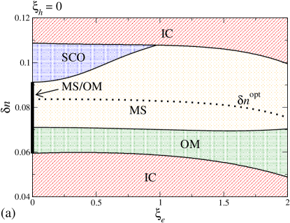
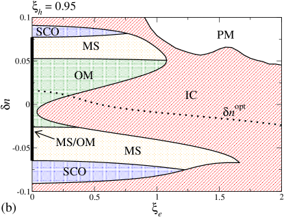
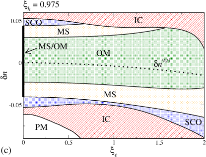
Figure 2: (color online) Magnetic order at $T=T_{N}^{-}$ as a function of $\xi_{e}$ and $\delta{n}$ for (a) $\xi_{h}=0$, (b) $\xi_{h}=0.95$, and (c) $\xi_{h}=0.975$. Magnetic phases are as defined in the text. At $\xi_{e}=0$ the thick solid line indicates degenerate MS and OM solutions. For $\xi_{e}\neq 0$, solid lines indicate phase boundaries, while the dotted line indicates the optimal doping $\delta{n}^{\text{opt}}$.

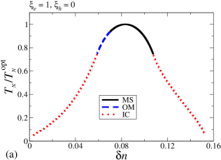
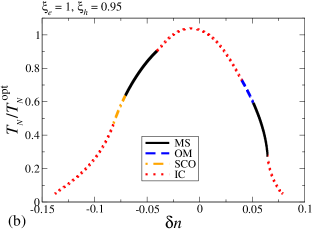
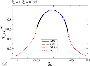
Figure 3: (color online) Critical temperature $T_{N}$ of the SDW states as a function of doping $\delta{n}$ for $\xi_{e}=1$ and (a) $\xi_{h}=0$, (b) $\xi_{h}=0.95$, and (c) $\xi_{h}=0.975$. The temperature is scaled by the maximum temperature for commensurate SDW order $k_{B}T^{\text{opt}}_{N}=0.0646\,t_{c}$.

The free energy in Eq. (LABEL:eq:freeE) allows us to determine the phase diagram of the model close to $T_{N}$. In Fig. 2 we present phase diagrams showing the ordered state realized at a temperature $T=T_{N}^{-}$ infinitesimally below $T_{N}$ as a function of $\xi_{e}$ and of the doping relative to half-filling, $\delta{n}$, for various values of $\xi_{h}$. In constructing the phase diagrams, we adjust $g_{\text{SDW}}$ such that for each value of $\xi_{e}$ the maximum critical temperature of the commensurate SDW as a function of the doping $\delta{n}$ is $k_{B}T^{\text{opt}}_{N}=0.0646\,t_{c}$, which gives a reasonable ratio of $k_{B}T^{\text{opt}}_{N}$ to the bandwidth. The variation of the optimal doping level $\delta{n}^{\text{opt}}$, where $T_{N}$ is maximal, with $\xi_{e}$ is shown by black dotted lines. The boundaries between the different commensurate SDW phases are determined by the conditions on the $\beta_{0}$, $\beta_{1}$ and $\widetilde{\beta}_{2}$ mentioned above, where the coefficients in Eq. (6) were evaluated for $g_{1}=g_{2}$ and using a $1000\times 1000$ ${\bf k}$-point mesh. In all phase diagrams we find regions where IC SDW order occurs. Since the IC SDW ordering vector is likely close to the commensurate SDW vector, Schmiedt2011 the boundary between the two phases is determined by solving $1+(g_{\text{SDW}}/V)\sum_{\bf k}(1/\beta)\sum_{n}G^{c(0)}({\bf k},i\omega_{n})G^{f(0)}({\bf k}+{\bf Q}_{1}+{\bf\delta{q}},i\omega_{n})=0$ for the critical temperature of the ${\bf Q}_{1}+\delta{\bf q}$ SDW state, where $\delta{\bf q}=(0.01\pi/a,0)$, $(0,0.01\pi/a)$. When the critical temperature of the ${\bf Q}_{1}+\delta{\bf q}$ SDW exceeds that of the commensurate SDW, an IC SDW is assumed to be realized. We similarly find the critical doping for which there is no IC SDW order, and the system remains paramagnetic (PM) down to zero temperature. Note that we disregard states with $T_{N}<0.05\,T^{\text{opt}}_{N}$.

We first consider the phase diagram for $\xi_{h}=0$ [Fig. 2(a)], which corresponds to a Fermi surface with a single hole pocket and two electron pockets at optimal doping as shown in Fig. 1(b). A commensurate SDW state is realized here for $\delta{n}\approx\delta{n}^{\text{opt}}\pm 0.025$ for all $\xi_{e}$. At $\xi_{e}=0$ the condition $\epsilon^{f}_{\bf k}=\epsilon^{f}_{{\bf k}+{\bf Q}_{3}}$ is satisfied, and hence the OM and MS states are degenerate. These states have the lowest free energy at underdoping and near optimal doping, but at overdoping the SCO is realized. Upon switching on a finite $\xi_{e}$, the degeneracy of the MS and OM states is lifted, and the MS state is found to have the lower free energy near optimal doping and at overdoping, while the OM state is stable at underdoping. The SCO state is rapidly suppressed by a finite $\xi_{e}$.

The phase diagrams for the case of two hole and two electron Fermi pockets [see Fig. 1(c)] is shown in Figs. 2(b) and (c) for $\xi_{h}=0.95$ and $\xi_{h}=0.975$, which correspond to hole pockets of lesser and greater similarity, respectively. We note that the interaction strength $g_{\text{SDW}}$ needed to produce the SDW state is roughly a third smaller than for the single-hole-pocket scenario. For small $\xi_{e}$, a commensurate SDW is nevertheless realized over a much greater doping range than in the single-hole-pocket case. The OM phase is stable near optimal doping, with the MS phase found at moderate doping, and the SCO found at stronger doping. At larger values of $\xi_{e}$, however, we find a strong tendency towards IC order in the $\xi_{h}=0.95$ case, with commensurate order completely absent for $\xi_{e}>1.75$. In contrast, the commensurate SDW in the $\xi_{h}=0.975$ case is present for all $\xi_{e}$ and is always realized about optimal doping.

In Fig. 3 we plot the critical temperature of the SDW states as a function of doping $\delta{n}$ for constant-$\xi_{e}$ cuts through the three phase diagrams in Fig. 2. For the $\xi_{h}=0$ case [Fig. 3(a)] we note that there are substantial IC SDW “shoulders” to the commensurate SDW dome, which extend up to $T\approx 0.75\,T^{\text{opt}}_{N}$. Although IC SDW states are also found at strong underdoping or overdoping in the $\xi_{h}=0.975$ case [Fig. 3(c)], they are realized over a smaller doping range relative to the commensurate states and do not extend to such high temperatures compared to the single-hole-pocket scenario. As shown in Fig. 3(b), however, slightly reducing $\xi_{h}$ leads to IC states appearing at optimal doping.

V Discussion

To summarize our main results, we have shown that in a two-band model of the pnictides there are three distinct commensurate SDW states: The MS, OM, and SCO phases. In a model with a single hole pocket and two electron pockets, the MS state dominates the phase diagram, but the OM and SCO phases are possible away from optimal doping. For a model with two hole pockets, in contrast, the OM phase is stable at optimal doping, although the MS phase remains at under- and overdoping. Since only the MS state is observed experimentally, we hence conclude that the model with a single hole pocket gives a more reasonable description of the physics. We nevertheless note that such a model displays a rather strong tendency towards IC SDW order, which is not observed experimentally. Pratt2011

We consider the results for the single-hole-pocket case in more detail. In agreement with LABEL:EC2010 we found that MS order was realized near optimal doping for arbitrarily small ellipticity of the electron Fermi pockets. Away from optimal doping, however, states consisting of a superposition of commensurate SDWs with orthogonal ordering vectors ${\bf Q}_{1}$, ${\bf Q}_{2}$ are realized. This can be understood via the following argument. At strong underdoping, we expect that the best nesting between the hole pocket and the elliptical electron pockets occurs for the states near the major axis of the electron pockets, as shown in Fig. 4(a). Similarly, for strong overdoping the best nesting occurs for the states near the minor axis of the electron pockets [Fig. 4(c)]. In both cases, the SDW gaps for the two nesting vectors involve states far apart on the hole Fermi surface, and so there should be little competition between them. Near optimal doping, however, the nested electron Fermi pockets compete for the same states on the hole Fermi surface [Fig. 4(b)], and hence it is more favorable for only a single electron pocket to participate in the SDW. We note that the variation of the nesting “hotspots” with doping is expected to have significant consequences for the $a$-$b$ resistivity anomaly in the pnictides. Fernandes2011

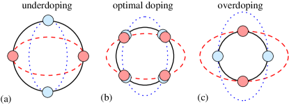
Figure 4: (color online) Schematic diagram of the nesting of the two electron pockets (blue dotted and red dashed lines) with a single hole pocket (black solid line). We show the situation for (a) underdoping, (b) optimal doping, and (c) overdoping. The small shaded circles indicate the region of best nesting of the electron pockets with the hole pocket.

The addition of a second hole pocket at the M point strongly affects the physics. The doping range of commensurate SDW states is significantly expanded, and the OM state is realized near optimal doping with a MS phase appearing upon doping. This is consistent with previous investigations of the two-orbital model. Lorenzana2008 ; Raghuvanishi2011 In contrast, our results are inconsistent with the degenerate OM and MS phases found in LABEL:EC2010. This is due to the fact that in the model of LABEL:EC2010 the $\Gamma$ hole pocket is mapped exactly onto the M pocket by translation of ${\bf Q}_{3}$, i.e., the degeneracy condition $\epsilon^{c}_{{\bf k}}=\epsilon^{c}_{{\bf k}+{\bf Q}_{3}}$ is always satisfied. Despite the apparent differences, the phase diagram can be understood in a similar way to the single-hole-pocket case. At optimal doping the nesting of the electron pockets is not optimal for either hole pocket, but instead corresponds to overdoping for the smaller pocket and underdoping for the larger pocket, thus allowing the OM phase. Indeed, this perfectly describes the nesting properties of the two-orbital model at half-filling. Brydon2011 Upon doping the system, the nesting with one of the hole pockets is optimized, while the nesting is the other hole pocket becomes extremely poor. As such, only a single hole pocket participates in the nesting, and so the MS state is stable. The relative size of the two hole pockets is thus crucial: If the two pockets are too dissimilar in size, there will be a tendency for the $T_{N}(\delta n)$ curves in Fig. 3 to split into two separate domes with commensurate order near their maxima. The strong tendency towards an IC SDW state at optimal doping suggests that the $\xi_{h}=0.95$ case is close to this limit. For somewhat lower $\xi_{h}$, i.e., when the hole pocket at the M point is much smaller than the pocket at the $\Gamma$ point, the pocket at the M point only shows good nesting with the electron pockets at very large hole doping. At realistic doping levels, the smaller hole pocket is essentially irrelevant for the SDW formation and the single-hole-pocket model is applicable.

Finally, we consider the implications of our results for the hypothesized nematic state in the pnictides. Indeed, a major motivation for our study is the connection of this phase with the MS SDW state. Fang2008 ; Kim2011 ; Fernandes2010 This can be seen via the following naive argument: After integrating out the CDW, we write the free energy Eq. (LABEL:eq:freeE) in terms of the sublattice magnetizations ${\bf m}_{a}$ and ${\bf m}_{b}$,

$$F = F_{0}+\frac{1}{2}\alpha\left(|{\bf m}_{a}|^{2}+|{\bf m}_{b}|^{2}\right)$$ (8)

$${}+\frac{1}{16}(2\beta_{0}+\beta_{1})\left(|{\bf m}_{a}|^{2}+|{\bf m}_{b}|^{2}\right)^{2}$$

$${}+\frac{1}{4}(2\beta_{0}-\beta_{1})\left({\bf m}_{a}\cdot{\bf m}_{b}\right)^{2}$$

$${}+\frac{1}{16}\widetilde{\beta}_{2}\left(|{\bf m}_{a}|^{2}-|{\bf m}_{b}|^{2}\right)^{2}\,,$$

and identify the Ising nematic degree of freedom as $\varphi={\bf m}_{a}\cdot{\bf m}_{b}$. In the mean-field theory presented in this paper, $\varphi$ is only non-zero in the MS phase. The inclusion of sufficiently strong magnetic fluctuations, however, allows the nematic order parameter to be non-zero above $T_{N}$,Fang2008 ; Kim2011 ; Fernandes2010 so long as the coefficient of $\varphi^{2}$ in Eq. (8) is negative, i.e $2\beta_{0}<\beta_{1}$. This is the same condition that ensures that the MS phase has lower free energy than the OM phase, and hence implies that a nematic transition occurs at $T\geq T_{N}$ when the SDW state shows stripe order. It is therefore intriguing that we find that $2\beta_{0}-\beta_{1}$ changes sign as a function of doping in all cases. This suggests a strong doping dependence of the nematic phase: In particular, for a scenario with a single hole pocket we expect that the nematic phase at underdoping will be weaker and occur closer to $T_{N}$ compared to overdoping, or may even be absent. Since this is apparently not observed experimentally, our results might imply that the magnetoelastic coupling plays a more direct role in the structural transition. magph

VI Summary

In this paper we have presented a weak-coupling study of the magnetic order in a two-band model of the iron pnictides. Using the Dyson equation for the Green’s function of an arbitrary commensurate SDW state treated at the mean-field level, we have obtained an expansion of the free energy valid close to the critical temperature. We have shown that this allows three commensurate SDW states: The experimentally relevant stripe MS phase, the flux OM phase, and the SCO phase for which only one sublattice orders. The competition of these phases with one another and with IC SDW states has been studied as a function of the doping and the variation of key features of the non-interacting electronic structure.

In particular, we have examined systems containing two elliptical electron pockets and either a single hole pocket at the $\Gamma$ point or hole pockets at both the $\Gamma$ and the M points. In the former case we find that the MS state is stable at optimal doping, while a superposition of two orthogonal SDW states is stable away from optimal doping. In the latter scenario, however, the OM phase is realized near optimal doping, while the MS state is stable at moderate doping and the SCO state appears at higher doping levels. The doping dependence of the associated phase diagrams can be understood in terms of the changing nesting properties of the Fermi surface. Our results indicate that the single-hole-pocket model is in better agreement with experiments, presumably because any hole pocket at the M point in the real materials is small and poorly nested with the electron pockets. The single-hole-pocket picture also suggest that the proposed nematic state in the pnictides should be highly asymmetric with respect to electron vs. hole doping.

- (1) J. Paglione and R. L. Greene, Nature Physics 6, 645 (2010).
- (2) D. C. Johnston, Adv. Phys. 59, 803 (2010).
- (3) M. D. Lumsden and A. D. Christianson, J. Phys.: Condens. Matter 22, 203203 (2010).
- (4) Y. Kamihara, T. Watanabe, M. Hirano, and H. Hosono, J. Am. Chem. Soc. 130, 3296 (2008).
- (5) M. Rotter, M. Tegel, and D. Johrendt, Phys. Rev. Lett. 101, 107006 (2008).
- (6) J. Zhao, Q. Huang, C. de la Cruz, S. Li, J. W. Lynn, Y. Chen, M. A. Green, G. F. Chen, G. Li, Z. Li, J. L. Luo, N. L. Wang, and P. Dai, Nature Mater 7, 953 (2008); J. Zhao, Q. Huang, C. de la Cruz, J. W. Lynn, M. D. Lumsden, Z. A. Ren, J. Yang, X. Shen, X. Dong, Z. Zhao, and P. Dai, Phys. Rev. B 78, 132504 (2008).
- (7) Q. Huang, Y. Qiu, W. Bao, M. A. Green, J. W. Lynn, Y. C. Gasparovic, T. Wu, G. Wu, and X. H. Chen, Phys. Rev. Lett. 101, 257003 (2008); A. Jesche, N. Caroca-Canales, H. Rosner, H. Borrmann, A. Ormeci, D. Kasinathan, H. H. Klauss, H. Luetkens, R. Khasanov, A. Amato, A. Hoser, K. Kaneko, C. Krellner, and C. Geibel, Phys. Rev. B 78, 180504(R) (2008).
- (8) C. Fang, H. Yao, W.-F. Tsai, J. P. Hu, and S. A. Kivelson, Phys. Rev. B 77 224509 (2008).
- (9) R. M. Fernandes, L. H. VanBebber, S. Bhattacharya, P. Chandra, V. Keppens, D. Mandrus, M. A. McGuire, B. C. Sales, A. S. Sefat, and J. Schmalian, Phys. Rev. Lett. 105, 157003 (2010).
- (10) M. G. Kim, R. M. Fernandes, A. Kreyssig, J. W. Kim, A. Thaler, S. L. Bud’ko, P. C. Canfield, R. J. McQueeney, J. Schmalian, and A. I. Goldman, Phys. Rev. B 83, 134522 (2011).
- (11) V. Barzykin and L. P. Gor’kov, Phys. Rev. B 79, 134510 (2009).
- (12) A. Cano, M. Civelli, I. Eremin, and I. Paul, Phys. Rev. B 82 020408(R) (2010); I. Paul, Phys. Rev. Lett. 107, 047004 (2011).
- (13) Q. Si and E. Abrahams, Phys. Rev. Lett. 101, 076401 (2008); T. Yildirim, Phys. Rev. Lett. 101, 057010 (2008); G. S. Uhrig, M. Holt, J. Oitmaa, O. P. Sushkov, and R. R. P. Singh, Phys. Rev. B 79, 092416 (2009).
- (14) F. Krüger, S. Kumar, J. Zaanen, and J. van den Brink, Phys. Rev. B 79, 054504 (2009); W. Lv, J. Wu, and P. Phillips, Phys. Rev. B 80, 224506 (2009).
- (15) M. A. McGuire, A. D. Christianson, A. S. Sefat, B. C. Sales, M. D. Lumsden, R. Jin, E. A. Payzant, D. Mandrus, Y. Luan, V. Keppens, V. Varadarajan, J. W. Brill, R. P. Hermann, M. T. Sougrati, F. Grandjean, G. J. Long, Phys. Rev. B 78, 094517 (2008); M. A. McGuire, R. P. Hermann, A. S. Sefat, B. C. Sales, R. Jin, D. Mandrus, F. Grandjean, and G. J. Long, New J. Phys. 11, 025011 (2009).
- (16) R. H. Liu, G. Wu, T. Wu, D. F. Fang, H. Chen, S. Y. Li, K. Liu, Y. L. Xie, X. F. Wang, R. L. Yang, L. Ding, C. He, D. L. Feng, and X. H. Chen, Phys. Rev. Lett. 101, 087001 (2008).
- (17) J. K. Dong, L. Ding, H. Wang, X. F. Wang, T. Wu, G. Wu, X. H. Chen, and S. Y. Li, New J. Phys. 10, 123031 (2008).
- (18) W. L. Yang, A. P. Sorini, C.-C. Chen, B. Moritz, W.-S. Lee, F. Vernay, P. Olalde-Velasco, J. D. Denlinger, B. Delley, J.-H. Chu, J. G. Analytis, I. R. Fisher, Z. A. Ren, J. Yang, W. Lu, Z. X. Zhao, J. van den Brink, Z. Hussain, Z.-X. Shen, and T. P. Devereaux, Phys. Rev. B 80, 014508 (2009).
- (19) D. K. Pratt, M. G. Kim, A. Kreyssig, Y. B. Lee, G. S. Tucker, A. Thaler, W. Tian, J. L. Zarestky, S. L. Bud’ko, P. C. Canfield, B. N. Harmon, A. I. Goldman, R. J. McQueeney, Phys. Rev. Lett. 106, 257001 (2011).
- (20) D. J. Singh and M.-H. Du, Phys. Rev. Lett. 100, 237003 (2008); I. I. Mazin, D. J. Singh, M. D. Johannes, and M. H. Du, ibid 101, 057003 (2008).
- (21) Y.-Z. Zhang, I. Opahle, H. O. Jeschke, and R. Valentí, Phys. Rev. B 81, 094505 (2010).
- (22) S. E. Sebastian, J. Gillett, N. Harrison, P. H. C. Lau, C. H. Mielke, and G. G. Lonzarich, J. Phys: Condens. Matter 20, 422203 (2008); J. G. Analytis, R. D. McDonald, J.-H. Chu, S. C. Riggs, A. F. Bangura, C. Kucharczyk, M. Johannes, and I. R. Fisher, Phys. Rev. B 80, 064507 (2009).
- (23) M. Yi, D. H. Lu, J. G. Analytis, J.-H. Chu, S.-K. Mo, R.-H. He, M. Hashimoto, R. G. Moore, I. I. Mazin, D. J. Singh, Z. Hussain, I. R. Fisher, and Z.-X. Shen, Phys. Rev. B 80, 174510 (2009); T. Shimojima, K. Ishizaka, Y. Ishida, N. Katayama, K. Ohgushi, T. Kiss, M. Okawa, T. Togashi, X.-Y. Wang, C.-T. Chen, S. Watanabe, R. Kadota, T. Oguchi, A. Chainani, and S. Shin , Phys. Rev. Lett. 104, 057002 (2010).
- (24) L. V. Keldysh and Y. V. Kopaev, Fiz. Tverd. Tela (Leningrad) 6, 2791 (1964) [Sov. Phys. Solid State 6, 2219 (1965)]; J. des Cloizeaux, J. Phys. Chem. Solids 26, 259 (1965); D. Jérome, T. M. Rice, and W. Kohn, Phys. Rev. 158, 462 (1967).
- (25) D. W. Buker, Phys. Rev. B 24, 5713 (1981).
- (26) T. M. Rice, Phys. Rev. B 2, 3619 (1970).
- (27) E. Fawcett, Rev. Mod. Phys. 60, 209 (1988).
- (28) S. Raghu, X.-L. Qi, C.-X. Liu, D. J. Scalapino, and S.-C. Zhang, Phys. Rev. B 77, 220503(R) (2008).
- (29) J. Lorenzana, G. Seibold, C. Ortix, and M. Grilli, Phys. Rev. Lett. 101, 186402 (2008).
- (30) N. Raghuvanishi and A. Singh, J. Phys.:Condens. Matter 23, 312201 (2011).
- (31) J. Knolle, I. Eremin, and R. Moessner, Phys. Rev. B 83, 224503 (2011).
- (32) A. Nicholson, Q. Luo, W. Ge, J. Riera, M. Daghofer, G. B. Martins, A. Moreo, E. Dagotto, Phys. Rev. B 84, 094519 (2011).
- (33) K. Kuroki, S. Onari, R. Arita, H. Usui, Y. Tanaka, H. Kontani, and H. Aoki, Phys. Rev. Lett. 101, 087004 (2008).
- (34) S. Graser, T. A. Maier, P. J. Hirschfeld, and D. J. Scalapino, New J. Phys. 11, 025016 (2009).
- (35) P. M. R. Brydon, M. Daghofer, and C. Timm, J. Phys.: Condens. Matter 23, 246001 (2011).
- (36) J. Schmiedt, P. M. R. Brydon, and C. Timm, arXiv:1108.5296 (unpublished).
- (37) A. V. Chubukov, D. V. Efremov, and I. Eremin, Phys. Rev. B 78, 134512 (2008).
- (38) P. M. R. Brydon and C. Timm, Phys. Rev. B 79, 180504(R) (2009).
- (39) V. Cvetkovic and Z. Tesanovic, Europhys. Lett. 85, 37002 (2009); Phys. Rev. B 80, 024512 (2009).
- (40) C. Platt, C. Honerkamp, and W. hanke, New J. Phys. 11, 055058 (2009).
- (41) A. B. Vorontsov, M. G. Vavilov, and A. V. Chubukov, Phys. Rev. B 79, 060508(R) (2009); Phys. Rev. B 81, 174538 (2010).
- (42) P. M. R. Brydon and C. Timm, Phys. Rev. B 80, 174401 (2009).
- (43) I. Eremin and A. V. Chubukov, Phys. Rev. B 81, 024511 (2010).
- (44) J. Knolle, I. Eremin, A. V. Chubukov, and R. Moessner, Phys. Rev. B 81, 140506(R) (2010).
- (45) R. M. Fernandes and J. Schmalian, Phys. Rev. B 82, 014521 (2010).
- (46) J. Knolle, I. Eremin, A. Akbari, and R. Moessner, Phys. Rev. Lett. 104, 257001 (2010); A. Akbari, J. Knolle, I. Eremin, and R. Moessner, Phys. Rev. B 82, 224506 (2010).
- (47) S. Maiti and A. V. Chubukov, Phys. Rev. B 82, 214515 (2010).
- (48) J. Kang and Z. Tešanović, Phys. Rev. B 83, 020505(R) (2011).
- (49) B. Zocher, C. Timm, and P. M. R. Brydon, Phys. Rev. B 84, 144425 (2011).
- (50) J. Knolle, I. Eremin, J. Schmalian, and R. Moessner, Phys. Rev. B 84, 180510(R) (2011).
- (51) A. V. Balatsky, D. N. Basov, and J. X. Zhu, Phys. Rev. B 82, 144522 (2010).
- (52) J. C. Tolédano and P. Tolédano, The Landau Theory of Phase Transitions (World Scientific, Singapore, 1987).
- (53) R. M. Fernandes, E. Abrahams, and J. Schmalian, Phys. Rev. Lett. 107, 217002 (2011).