Signatures of Rashba spin-orbit interaction in the superconducting proximity effect in helical Luttinger liquids

Abstract

We consider the superconducting proximity effect in a helical Luttinger liquid at the edge of a 2D topological insulator, and derive the low-energy Hamiltonian for an edge state tunnel-coupled to a $s$-wave superconductor. In addition to correlations between the left and right moving modes, the coupling can induce them inside a single mode, as the spin axis of the edge modes is not necessarily constant. This can be induced controllably in HgTe/CdTe quantum wells via the Rashba spin-orbit coupling, and is a consequence of the 2D nature of the edge state wave function. The distinction of these two features in the proximity effect is also vital for the use of such helical modes in order to split Cooper-pairs. We discuss the consequent transport signatures, and point out a long-ranged feature in a dc conductance measurement that can be used to distinguish the two types of correlations present and to determine the magnitude of the Rashba interaction.

I Introduction

The helical edge states of a 2D topological insulator (TI) consist of a Kramers pair of right- and left-moving electron modes of opposite spin situated inside the bulk gap Kane and Mele (2005); Bernevig et al. (2006); Wu et al. (2006); Xu and Moore (2006), and they have so far been observed in HgTe/CdTe quantum wells (HgTe-QW) Bernevig et al. (2006); König et al. (2007); Roth et al. (2009). In 3D topological insulators, the edge states cover the surface of the material and consist of a single-valley Dirac cone with spin-momentum locking, which leads to unique electromagnetic properties and quantum interference effects Qi and Zhang (2011); *hasan2010-cti. In both 2D-TI and 3D-TI the coupling of spin and orbital motion can lead to interesting effects when combined with superconductivity. Superconducting correlations induced by the proximity of a singlet $s$-wave superconductor can inside the TI obtain a $p$-wave character, which can be used to engineer Majorana bound states. Fu and Kane (2008); Linder et al. (2010); Stanescu et al. (2010) A somewhat similar induction of non-conventional correlations has also been proposed to occur in other semiconductor systems in the combined presence of the spin-orbit interaction and superconductivity. Sau et al. (2010a); *sau2010-rom; *alicea2010-mfi; *linder2010-mfm

When the edge state of a 2D-TI is coupled to a singlet superconductor, the transfer of electrons between the systems can, first of all, induce singlet-type proximity correlations between electrons in the right and left moving modes (the $+-$ channel). Fu and Kane (2008) This already leads to several effects of interest. For instance, the helicity of the electron liquid lifts the spin degeneracy and enables Majorana states, Fu and Kane (2009) causes Cooper pairs to split, Sato et al. (2010) and affects transport properties. Adroguer et al. (2010) Tight-binding calculations studying the pair amplitude have also been made Black-Schaffer (2011). There is, however, also a possibility of inducing correlations only within the right-moving (or the left-moving) channel at a nonzero total momentum (the $++$ and $--$ channels). Such a channel is not forbidden by symmetries in the problem: due to the spin-orbit coupling, the spin axis of the edge state is not necessarily constant, so that the electrons forming a Cooper pair singlet can both enter the same mode on the TI edge, even when spin is conserved in the tunneling process and time-reversal symmetry is present. In HgTe-QW, a non-constant spin axis can be induced externally by the Rashba spin-orbit coupling that breaks inversion symmetry. Roth et al. (2009) Momentum conservation is required to be broken, but this can occur e.g. due to inhomogeneity or a finite size of a tunneling contact. Moreover, unlike in metals, in 2D-TI the momentum non-conservation can in principle be made arbitrarily small by tuning the Fermi level near the Dirac point ($k=0$).

A straightforward way to probe the existence of superconducting correlations is to observe the Josephson effect or other interference effects that can be modulated with superconducting phase differences. The Josephson effect has been studied previously in various one-dimensional Luttinger liquid systems. Fisher (1994); Fazio et al. (1996, 1995) The finite-momentum channel has, however, received limited attention, Pugnetti et al. (2007) and is usually negligible. As shown below, certain experiments with superconducting contacts attached to the helical edge states can nevertheless probe such microscopic aspects of the tunneling, including the role of the Rashba interaction.

Here, we first derive a low-energy Hamiltonian describing the superconducting proximity effect in the edge states of a 2D TI coupled to a conventional superconductor by tunnel contacts. We use it to find the signatures of both types of tunneling events in a transport experiment. Because of the reduced number of propagating modes in the helical liquid, correlations within the same channel occur at a finite momentum and, as in chiral liquids, Fisher (1994) are affected by the exclusion principle. It turns out that although this component of the proximity effect gives a negligible correction to the dc Josephson effect, in the NS tunneling conductance [see Fig. 1(c)] it manifests as a long-ranged interference effect, oscillating as a function of the superconducting phase difference, and unlike the $+-$ part, is not exponentially suppressed at length scales longer than the thermal wavelength. The ratio of the contributions of the two possible channels scales as $\delta G_{++}/\delta G_{+-}\propto{}(z_{0}/\hbar v_{F})^{2}(k_{B}T/M)^{2}e^{2\pi Td/\hbar v_{F}}$ (in the noninteracting case), where $z_{0}$ characterizes the strength of Rashba interaction, $v_{F}$ is the Fermi velocity of the edge channels, $M$ is the energy gap of the TI, and $d$ the distance between two superconducting contacts forming the interferometry setup. The amplitude of the effect is proportional to the amount of spin rotation achieved by Rashba interaction, and the quadratic temperature dependence is due to the exclusion principle. We also discuss how $e$-$e$ interactions modify this result.

This paper is organized as follows. In Section II, we introduce the model for the helical Luttinger liquid (HLL), the coupling to the superconductors, and the electronic structure of HgTe-QWs. Section III discusses the effective low-energy Hamiltonian, and Section IV transport signatures in the dc and ac Josephson effects and the NS conductance. Section V concludes the manuscript with a discussion on the results and remarks on experimental realizability.

II Model

We consider the setup depicted in Fig. 1. The edge states of a 2D-TI are coupled to two superconducting terminals via two tunnel junctions. Below, we in general assume that the distance $d$ between the contacts is longer than the superconducting coherence length $\xi$.

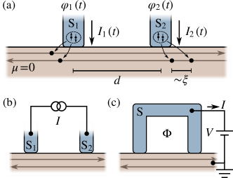
Figure 1: (a) The setup considered: a 2D topological insulator, whose edge state is coupled to two superconductors via tunnel contacts. In response to phase $\varphi$ or voltage $V$ differences between the superconductors, Josephson currents can flow via the edge channel, or one can probe the NS transmission by injecting current from the superconductors to the edge channel. If the spin axis of the edge state is not constant spatially and as a function of energy, a Cooper pair singlet can enter the edge state in two possible ways: either electrons enter modes propagating to opposite directions (left) or the same direction (right). In the latter case, exclusion principle requires temporal (or spatial) separation of the two, which can be of the order of the superconducting coherence length $\xi=\hbar v_{F}/\Delta$ still preserving the correlation. (b) Configuration for the measurement of the Josephson current. (c) Configuration for the measurement of interference in the NS conductance.

The left- and right moving edge states $\lvert{+,x}\rangle$ and $\lvert{-,x}\rangle$ have a linear dispersion, and are described by the bosonized Hamiltonian Wu et al. (2006)

$$H_{0}=\frac{1}{2}\int_{-\infty}^{\infty}\mathrm{d}x\,u[g^{-1}(\partial_{x}\vartheta)^{2}+g(\partial_{x}\phi)^{2}]$$ (1)

where the Fermi field operator is $\psi_{\alpha}(x)=(2\pi a_{0})^{-1/2}U_{\alpha}e^{i\alpha k_{F}x}e^{i\phi_{\alpha}(x)}=(2\pi a_{0})^{-1/2}U_{\alpha}e^{i\alpha[k_{F}x+\sqrt{\pi}\vartheta(x)]+i\sqrt{\pi}\phi(x)}$, the standard boson fields $\vartheta(x)$, $\phi(x)$ satisfy $[\phi(x),\vartheta(x^{\prime})]=(i/2)\mathop{\mathrm{sgn}}(x-x^{\prime})$, and $U_{\pm}$ are the Klein factors. $u=v_{F}/g$ is the renormalized Fermi velocity. Here and below, we let $\hbar=k_{B}=e=1$, unless otherwise mentioned. The parameter $a_{0}$ is the short-distance cutoff. In the noninteracting case, the Luttinger interaction parameter $g=1$, and with repulsive electron-electron interactions one has $g<1$.

The coupling to the superconductors is modeled with a tunneling Hamiltonian

$$H_{T}=\sum_{\alpha=\pm,\sigma^{\prime}=\uparrow,\downarrow}\int\mathrm{d}x\,\mathrm{d}^{3}r^{\prime}\,t_{\alpha\sigma^{\prime}}(x,\vec{r}^{\prime})\psi^{\dagger}_{\alpha}(x)\psi_{S\sigma^{\prime}}(\vec{r}^{\prime})+\mathrm{h.c.}\,,$$ (2)

where the tunneling amplitude $t_{\alpha\sigma^{\prime}}(x,\vec{r}^{\prime})$ describes the tunneling from the state $\lvert{\sigma^{\prime},\vec{r}^{\prime}}\rangle$ in the superconductor to state $\lvert{\alpha,x}\rangle$ in the edge mode. For what follows, it is useful to introduce also the corresponding one-particle operator $\hat{h}_{T}$, in terms of which, $t_{\alpha\sigma^{\prime}}(x,\vec{r}^{\prime})\equiv{}\langle{\alpha,x}\rvert\hat{h}_{T}\lvert{\sigma^{\prime},\vec{r}^{\prime}}\rangle$  . The momentum $k$ along the edge is a good quantum number for straight TI edges, and we define the state $\lvert{\alpha,x}\rangle$ in the momentum representation: $\lvert{\alpha,x}\rangle=\sum_{k}e^{-ikx}\lvert{\alpha,k}\rangle$, where $\lvert{\alpha,k}\rangle$ is the edge eigenstate with momentum $k$ and propagation direction $\alpha=\pm$.

We assume that the Hamiltonian is time-reversal symmetric, which implies that the tunneling operator in general satisfies $\mathfrak{T}\hat{h}_{T}\mathfrak{T}^{-1}=\hat{h}_{T}$. Here, we choose the phases of the wave functions so that the time reversal operations read $\mathfrak{T}\lvert{\sigma^{\prime},\vec{r}^{\prime}}\rangle=\sigma^{\prime}\lvert{-\sigma^{\prime},\vec{r}^{\prime}}\rangle$ and $\mathfrak{T}\lvert{\alpha,k}\rangle=\alpha\lvert{-\alpha,-k}\rangle$. We also assume that the tunneling is spin-conserving, that is, written in terms of real electron spin states in the TI and the superconductor, we have $\langle{\sigma,\vec{r}}\rvert\hat{h}_{T}\lvert{-\sigma,\vec{r}^{\prime}}\rangle=0$.

To describe tunneling to HgTe-QWs, we need some knowledge of the structure of the edge states. This can be obtained from the four-band model used in Ref. Bernevig et al., 2006. In this approach, the low-energy properties of the TI are described using a 2D envelope function in the basis of four states $\{\lvert{E1+}\rangle,\lvert{H1+}\rangle,\lvert{E1-}\rangle,\lvert{H1-}\rangle\}$ localized in the quantum well. Bernevig et al. (2006); Novik et al. (2005) The edge states at the boundaries of the TI can be solved within this four-band model; Zhou et al. (2008) for which we give a full analytical solution in Appendix A.

We assume the terminals are conventional spin-singlet superconductors. As usual, Abrikosov et al. (1975) they are characterized by the correlation function $F(\vec{r}_{1},\sigma_{1},\tau_{1};\vec{r}_{2},\sigma_{2},\tau_{2})\equiv\langle{T[\psi_{\sigma_{1}}(\vec{r}_{1},\tau_{1})\psi_{\sigma_{2}}(\vec{r}_{2},\tau_{2})]}\rangle_{0}$ that has a singlet symmetry $F(\vec{r}_{1},\sigma_{1},\tau_{1};\vec{r}_{2},\sigma_{2},\tau_{2})=\sigma_{1}\delta_{\sigma_{1},-\sigma_{2}}F(\vec{r}_{1},\tau_{1};\vec{r}_{2},\tau_{2})$. In the bulk, the correlation function obtains its equilibrium BCS form, which in imaginary time can be written as

$$F(\vec{r}_{1},\vec{r}_{2};\omega)=\int\frac{\mathrm{d}^{3}k\,}{(2\pi)^{3}}e^{-i(\vec{r}_{1}-\vec{r}_{2})\cdot\vec{k}}\frac{\Delta}{\omega^{2}+\xi_{k}^{2}+|\Delta|^{2}}\,,$$ (3)

with $\xi_{k}=k^{2}/(2m)-\mu$ the dispersion relation and $\Delta$ the gap of the superconductor.

III Effective Hamiltonian

Integrating out the superconductors using perturbative renormalization group theory (RG) and considering only energies $|E|\ll|\Delta|$ reduces the Hamiltonian $H_{0}+H_{T}$ of the total system to one concerning only the one-dimensional edge states:

$$H =H_{0}+\int\mathrm{d}x\,[\Gamma_{+-}(x)\psi_{+}(x)\psi_{-}(x)$$ (4)

$$\qquad+\Gamma_{++}(x)\psi_{+}(x)\psi_{+}(x+a)$$

$$\qquad+\Gamma_{--}(x)\psi_{-}(x)\psi_{-}(x+a)+\mathrm{h.c.}]\,.$$

Here, $\Gamma_{\alpha\beta}$ describe the coupling to the superconductor, and $a=\hbar v_{F}/\Delta$ is the new short-distance cutoff in the theory. Details of the derivation are discussed in Appendix B.

The coupling factors in the noninteracting case ($g=1$) are given by the expressions (see Appendix B for general discussion):

$$\Gamma_{++}(x)=\frac{\pi}{2}\int\mathrm{d}^{3}r_{1}^{\prime}\,\mathrm{d}^{3}r_{2}^{\prime}\,\sum_{K}e^{iKx}F(r_{1}^{\prime},r_{2}^{\prime};0)$$ (5)

$$\times\Delta v_{F}^{-1}\partial_{k}P_{++}(\frac{K}{2}+k,r_{1}^{\prime};\frac{K}{2}-k,r_{2}^{\prime})^{*}\rvert_{k=0}\,,$$

where $F$ is given in Eq. (3), and

$$\Gamma_{+-}(x)=\pi\int\mathrm{d}^{3}r_{1}^{\prime}\,\mathrm{d}^{3}r_{2}^{\prime}\,\sum_{K}e^{iKx}F(r_{1}^{\prime},r_{2}^{\prime};0)$$ (6)

$$\times P_{+-}(\frac{K}{2}-k_{F},r_{1}^{\prime};\frac{K}{2}+k_{F},r_{2}^{\prime})^{*}\,,$$

with $\Gamma_{--}=\Gamma_{++}^{*}$ in the presence of time reversal symmetry. The main contributions should arise around $K=-2k_{F}$ for $\Gamma_{++}$ (due to the $2k_{F}$ oscillations in the Fermi operators), and around $K=0$ for $\Gamma_{+-}$.

The coupling is proportional to the factor

$$P_{\alpha_{1}\alpha_{2}}(k_{1},\vec{r}_{1}^{\prime};k_{2},\vec{r}_{2}^{\prime}) \equiv[t_{\alpha_{1}\downarrow}(k_{1},\vec{r}_{1}^{\prime})t_{\alpha_{2}\uparrow}(k_{2},\vec{r}_{2}^{\prime})$$ (7)

$$-t_{\alpha_{1}\uparrow}(k_{1},\vec{r}_{1}^{\prime})t_{\alpha_{2}\downarrow}(k_{2},\vec{r}_{2}^{\prime})]+[\vec{r}_{1}^{\prime}\leftrightarrow{}\vec{r}_{2}^{\prime}]\,,$$

which describes two-particle tunneling of a singlet, from two points $\vec{r}_{1}^{\prime}$ and $\vec{r}_{2}^{\prime}$ in the superconductor, to momentum states $\lvert{\alpha_{1},-k_{1}}\rangle$, $\lvert{\alpha_{2},-k_{2}}\rangle$ in the TI edge modes (cf. Fig. 2). Here, $t_{\alpha\sigma^{\prime}}(k,\vec{r}^{\prime})=\int\mathrm{d}x\,e^{ikx}t_{\alpha\sigma^{\prime}}(x,\vec{r}^{\prime})=\langle{\alpha,-k}\rvert\hat{h}_{T}\lvert{\sigma^{\prime},\vec{r}^{\prime}}\rangle$ is a Fourier transform of the tunneling matrix element.

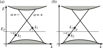
Figure 2: Schematic depiction of the edge mode spectrum and the states participating in 2-particle tunneling from the Fermi level in the superconductor to states in the TI. (a) In the $+-$ channel, the momenta corresponding to energy $\varepsilon$ are $k_{1}=k_{F}-\varepsilon/\hbar v_{F}$, $k_{2}=-k_{F}-\varepsilon/\hbar v_{F}$. (b) In the $++$ channel, one has $k_{1}=-k_{F}+\varepsilon/\hbar v_{F}$, $k_{2}=-k_{F}-\varepsilon/\hbar v_{F}$. Singlet pair tunneling into the $++$ channel can occur if the electron spin axis is different for the states at $k_{1}$ and $k_{2}$.

One can also verify that in the absence of interactions, the expression for the $\Gamma_{+-}$ amplitude coincides with the leading term in the zero-bias conductance in the normal state, up to a replacement $F\mapsto 2(\pi v_{F})^{-1}\mathop{\mathrm{Im}}G^{R}$. Within a quasiclassical approximation in the superconductor, Rammer and Smith (1986) one then finds a relation to the normal-state conductance per unit length, $g(x)$, of the tunnel interface:

$$\Gamma_{+-}(x)\simeq\frac{1}{4}\hbar v_{F}R_{K}g(x)=\frac{\hbar v_{F}}{l_{T}}\frac{R_{K}}{4R_{N}}\,.$$ (8)

Such a relation is typical for NS systems, and connects the amplitude $\Gamma_{+-}$ to observable quantities. The latter expression assumes the total resistance $R_{N}$ is uniformly distributed in a junction of length $l_{T}$. When the interface resistance decreases, the effective pairing amplitude $\Gamma$ grows — and although not included in our perturbative calculation, one expects that this increase is cut off when the effective gap reaches the bulk gap of the superconductor, $\Gamma_{+-}=\Delta$.

Unlike $\Gamma_{+-}$, the $\Gamma_{++/--}$ amplitudes do not have a direct relation to the normal-state conductance, and they depend on the factors $P_{++/--}$, which are proportional to the spin rotation between the states involved in the pair tunneling (see Fig. 2). Estimating this factor is necessary for determining how large the same-mode tunneling is in a given system.

III.1 Two-particle tunneling

Making use of the time-reversal symmetry, it is possible to rewrite the $P$ factors in a more transparent form:

$$P_{\alpha_{1}\alpha_{2}}(k_{1},\vec{r}_{1}^{\prime};k_{2},\vec{r}_{2}^{\prime})=\langle{\alpha_{1},-k_{1}}\rvert\hat{Z}(\vec{r}_{1}^{\prime},\vec{r}_{2}^{\prime})\mathfrak{T}\lvert{\alpha_{2},-k_{2}}\rangle\,,$$ (9)

$$\hat{Z}(\vec{r}_{1}^{\prime},\vec{r}_{2}^{\prime})\equiv\hat{h}_{T}[1_{\sigma}\otimes(\lvert{\vec{r}_{1}^{\prime}}\rangle\langle{\vec{r}_{2}^{\prime}}\rvert+\lvert{\vec{r}_{2}^{\prime}}\rangle\langle{\vec{r}_{1}^{\prime}}\rvert)]\hat{h}_{T}\,,$$ (10)

where $1_{\sigma}$ is the identity matrix in the spin space of the superconductor. Unlike the starting point, this expression is explicitly independent of the choice of the spin quantization axis. We also note the symmetry:

$$P_{\alpha_{1}\alpha_{2}}(k_{1},r_{1}^{\prime};k_{2},r_{2}^{\prime}) =-P_{\alpha_{2}\alpha_{1}}(k_{2},r_{1}^{\prime};k_{1},r_{2}^{\prime})\,,$$ (11)

following from the definition Eq. (7).

We can now make some remarks on the possibility of $++$ tunneling. First, suppose that the state $\lvert{\alpha,k}\rangle$ describes an electron wave function with a fixed $k$-independent and spatially constant spin part, and that the tunneling is spin conserving. In this case it is easy to see that $P_{++}=0$, as the inner product of a spinor and its time reversed counterpart vanishes. Such a situation is realized, for instance, within the plain Kane-Mele model. Kane and Mele (2005) Breaking such conditions can, however, lead to $P_{++}\neq 0$. We demonstrate in the next section that this can occur in HgTe-QW.

III.2 Effect of Rashba interaction in HgTe/CdTe quantum wells

We now discuss a simple model for tunneling into the helical edge states of a HgTe-QW, taking spin axis rotation from the Rashba interaction into account. We make the following assumptions: the tunneling is spin-conserving and local [$\langle{\vec{r}}\rvert\hat{h}_{T}\lvert{\vec{r}^{\prime}}\rangle\propto\delta(\vec{r}-\vec{r}^{\prime})$] on the length scales of the four-band model. This results to all contributions to $P_{++}$ coming solely from the Rashba mixing. While we cannot estimate the actual values of $P_{+-}$ or $P_{++}$ within this simplified a model, we can study their relative magnitudes, which is now determined by the low-energy four-band physics only.

Under the locality and spin-conservation assumptions, the tunnel matrix element introduced above obtains the following form in terms of envelope spinor wave functions $\hat{\Psi}$ in the four-band basis $\{\lvert{j}\rangle\}=\{\lvert{E1+}\rangle,\lvert{H1+}\rangle,\lvert{E1-}\rangle,\lvert{H1-}\rangle\}$:

$$\begin{split}P_{\alpha_{1}\alpha_{2}}(k_{1},\vec{r}_{1}^{\prime};k_{2},\vec{r}_{2}^{\prime})&=\hat{\Psi}_{\alpha_{1},-k_{1}}(x_{1}^{\prime},y_{1}^{\prime})^{\dagger}\hat{\cal Z}(\vec{r}_{1}^{\prime},\vec{r}_{2}^{\prime})\\ &\;\times\mathfrak{T}\hat{\Psi}_{\alpha_{2},-k_{2}}(x_{2}^{\prime},y_{2}^{\prime})+[\vec{r}_{1}^{\prime}\leftrightarrow\vec{r}_{2}^{\prime}]\,,\end{split}$$ (12)

$$\hat{\cal Z}(\vec{r}_{1}^{\prime},\vec{r}_{2}^{\prime})_{jj^{\prime}} =\langle{j}\rvert h_{T}[1_{\sigma}\otimes\lvert{\vec{r}_{1}^{\prime}}\rangle\langle{\vec{r}_{2}^{\prime}}\rvert]h_{T}\lvert{j^{\prime}}\rangle\,.$$ (13)

Time reversal for the four-band spinor reads $\mathfrak{T}=-i\tau_{y}K$ with $K$ the complex conjugation, and the $\tau$ matrix acts on the Kramers blocks ($+$, $-$). For simplicity, we use now a length-scale separation between the scales appearing in the four-band model ($\Psi$) and the atomic ones (tunneling ${\cal Z}$, $k_{F,S}$ in the superconductor, unit cell). We consider only the long-wavelength part of $P$, and replace ${\cal Z}$ with a constant describing the tunnel coupling to the quantum well basis states, obtained by averaging it together with $F$ [cf. Eqs. (5), (6)] over $\vec{r}_{1}^{\prime}$ and $\vec{r}_{2}^{\prime}$:

$$\overline{[{\cal Z}(\vec{r}_{1}^{\prime},\vec{r}_{2}^{\prime})+{\cal Z}(\vec{r}_{2}^{\prime},\vec{r}_{1}^{\prime})]F(\vec{r}_{1}^{\prime},\vec{r}_{2}^{\prime})}$$

$$\;\sim\begin{pmatrix}{\cal A}(\vec{r}_{1}^{\prime})&{\cal C}(\vec{r}_{1}^{\prime})&0&{\cal D}(\vec{r}_{1}^{\prime})\\ {\cal C}(\vec{r}_{1}^{\prime})^{*}&{\cal B}(\vec{r}_{1}^{\prime})&-{\cal D}(\vec{r}_{1}^{\prime})&0\\ 0&-{\cal D}(\vec{r}_{1}^{\prime})^{*}&{\cal A}(\vec{r}_{1}^{\prime})&{\cal C}(\vec{r}_{1}^{\prime})^{*}\\ {\cal D}(\vec{r}_{1}^{\prime})^{*}&0&{\cal C}(\vec{r}_{1}^{\prime})&{\cal B}(\vec{r}_{1}^{\prime})\end{pmatrix}F(0)\delta(\vec{r}_{1}^{\prime}-\vec{r}_{2}^{\prime})\,,$$ (14)

with ${\cal A}$ and ${\cal B}$ real-valued. This form follows from the time reversal symmetry and hermiticity of the matrix elements of the operator in Eq. (10). We have also assumed here that the decay length for the $F$ function ($\sim{}k_{F,S}^{-1}$) is short on the scales of the 4-band model. Finally, we for simplicity neglect the coupling to the $H1$ band, and set ${\cal B}={\cal C}=0$. For a lateral contact (SC on top of HgTe-QW), the main tunnel coupling is expected to involve the E1 band, which extends deeper Bernevig et al. (2006) into the CdTe barrier than H1. Including additional couplings would however cause no essential qualitative differences in the estimated ratio between the $++$ and $+-$ terms.

Without additional spin axis rotation from the Rashba interaction, the edge states are in separate Kramers blocks (see Appendix A), $\hat{\Psi}_{+}\propto{}(\hat{\Phi}_{+},0)$ and $\hat{\Psi}_{-}\propto{}(0,\hat{\Phi}_{-})$, and we can see that $P_{++}=0$ whereas $P_{+-}\propto{}{\cal A}$. Note that a contribution proportional ${\cal D}$ does not arise: the unperturbed edge state wave functions are both proportional to the same constant real-valued spinor, $\hat{\Phi}_{\pm}\propto\hat{\chi}$, so that the ${\cal D}$-dependent contribution would be proportional to $\hat{\chi}^{\dagger}i\sigma_{y}\hat{\chi}=0$. This structure also implies that contributions proportional to ${\cal D}$ do not arise in the leading order of the Rashba coupling.

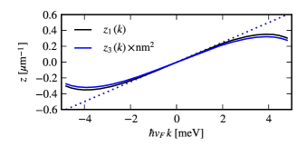
Figure 3: Projections $z(k)$ of the additional spin-orbit couplings $R_{0}$ and $T_{0}$ on the edge state basis, for the parameters of Ref. Rothe et al., 2010 with $M=-10\,\mathrm{meV}$. The dashed lines indicate linear approximations $z_{1}\approx{}z_{0,1}k$ and $z_{3}\approx{}z_{0,3}k$ with $z_{0,1}=0.03$ and $z_{0,3}=0.03\mathrm{nm^{-2}}$.

Rashba and other related spin-orbit interactions in the four-band model can be represented as Rothe et al. (2010)

$$H_{R}=\begin{pmatrix}0&h_{R}\\ h_{R}^{\dagger}&0\end{pmatrix}\,,\quad h_{R}=i\begin{pmatrix}-R_{0}k_{-}&\delta+iS_{0}k_{-}^{2}\\ -\delta-iS_{0}k_{-}^{2}&T_{0}k_{-}^{3}\end{pmatrix}\,,$$ (15)

where $k_{\pm}=k\pm ik_{y}$. For the QW parameters used in Ref. Rothe et al., 2010, $R_{0}\approx-15.6\,\mathrm{nm^{2}}\times eE_{z}$, $iS_{0}\approx-2.10\,\mathrm{nm^{3}}\times eE_{z}$, and $T_{0}\approx{}-8.91\,\mathrm{nm^{4}}\times eE_{z}$, where $E_{z}$ is the electric field perpendicular to the QW plane. The model could also include the bulk inversion asymmetry terms $\delta$. König et al. (2008)

To obtain the effect of the Rashba interaction on the wave functions, we find the low-energy eigenstates of $H=H_{0}+H_{R}$ numerically. For given $k$, this is a 1-D eigenvalue problem in the $y$-direction, which can be discretized and solved by standard approaches. Analytical results can be obtained by perturbation theory in $H_{R}$ restricted to the low-energy subspace spanned by the unperturbed edge states. For typical experimental parameters, the whole wave functions $\hat{\Psi}$ however turn out to have a significant component also in the continuum of bulk modes above the gap, which is not adequately captured by such an approach. Our estimates for the matrix elements $P_{\alpha\beta}$ below are therefore based on the numerical solutions for the eigenstates.

However, qualitative understanding can be obtained on the basis of the model restricted to the low-energy subspace. Projecting $H_{R}$ to this basis (see Appendix A), we find the effective low-energy Hamiltonian of the system

$$H_{R}^{\prime} =\begin{pmatrix}0&-i[R_{0}w_{1}(k)+T_{0}w_{3}(k)]\\ \mathrm{c.c.}&0\end{pmatrix}\,,$$ (16)

$$w_{1}(k) =\chi_{1}^{2}\int_{-\infty}^{\infty}\mathrm{d}y\,f_{+,k}(y)[k+\partial_{y}]f_{-,k}(y)$$ (17)

$$w_{3}(k) =\chi_{2}^{2}\int_{-\infty}^{\infty}\mathrm{d}y\,f_{+,k}(y)[k+\partial_{y}]^{3}f_{-,k}(y)\,,$$ (18)

where $\hat{\Phi}_{\pm,k}(y)=f_{\pm,k}(y)\hat{\chi}$. This result is valid to the leading order in $h_{R}$. The constant and quadratic in $k$ terms (proportional to $\delta$ and $S_{0}$) give no contribution, as $\hat{\chi}^{\dagger}\sigma_{y}\hat{\chi}=0$. Using typical HgTe-QW parameters, Rothe et al. (2010) the integrals evaluate to $w_{1}(k)\approx{}w_{0,1}k$ and $w_{3}(k)\approx{}w_{0,3}k$ near the Dirac point, as illustrated in Fig. 3. The prefactor $w_{0,1}\approx{}0.03$ is essentially independent of the mass parameter $M$, and $w_{0,3}\approx{}0.03\mathrm{nm^{-2}}\times(|M|/10\,\mathrm{meV})$. Note here that the matrix element $0.03R_{0}k$ of the Rashba interaction with the edge states is significantly smaller than the $R_{0}k_{\pm}$ appearing in the bulk Hamiltonian. The $2\times 2$ effective Hamiltonian yields the wave functions:

$$\hat{\Psi}_{+,k}\simeq\begin{pmatrix}\hat{\Phi}_{+,k}\\ \frac{iw_{0}}{2v_{F}}\hat{\Phi}_{-,k}\end{pmatrix}\,,\quad\hat{\Psi}_{-,k}\simeq\begin{pmatrix}\frac{iw_{0}}{2v_{F}}\hat{\Phi}_{+,k}\\ \hat{\Phi}_{-,k}\end{pmatrix}\,,$$ (19)

where $w_{0}=R_{0}w_{0,1}+T_{0}w_{0,3}$. The Rashba interaction mixes the two Kramers blocks, but in the leading order does not modify the energy dispersion. Although the mixing angle of the $\hat{\Phi}_{\pm,k}$ spinors is independent of $k$, the total four-band spinor is not: the decay lengths $1/\lambda_{1/2}(k,\alpha)$ of $\hat{\Phi}_{\pm,k}$ in the $y$-direction depend on $k$ and are different for the $\alpha=+$ and $\alpha=-$ states: time-reversal symmetry only guarantees $\lambda_{1/2}(k,+)=\lambda_{1/2}(-k,-)$. This makes the electron spin axis to rotate both spatially and with energy $\varepsilon$, which ultimately is required for a finite $P_{++}$.

For comparison, we show in Fig. 4 the $E1-$ component of the numerically computed total edge state wave function $\Psi_{+,k}(y)$, and its projection to the low-energy subspace, which can be seen to match Eqs. (19) to a very good accuracy. The $E1-$ component is proportional to the Rashba coupling and contributes to $P_{++}$. As is clearly visible in the figure, neglecting the bulk states underestimates the total amount of spin rotation, for experimentally relevant parameters. For a larger (but unphysical) value for the gap $|M|$, the low-energy theory works slightly better, as visible in the inset of Fig. 4.

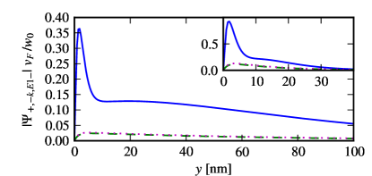
Figure 4: The $E1-$ component of $|\Psi_{+,-k}|$ at $k=|M|/(6\hbar v_{F})$. It is linear in the Rashba parameter $w_{0}/v_{F}$, provided $|w_{0}/v_{F}|\lesssim{}1$. Shown are numerical results (solid line), the component in the unperturbed edge state subspace (dashed line), and the result of Eq. (19) (dotted). The behavior for $y\gtrsim{}20\,\mathrm{nm}$ depends mainly on the linear in $k$ Rashba term $R_{0}$. Here, $M=-10\,\mathrm{meV}$. Inset: results for $M=-50\,\mathrm{meV}$.

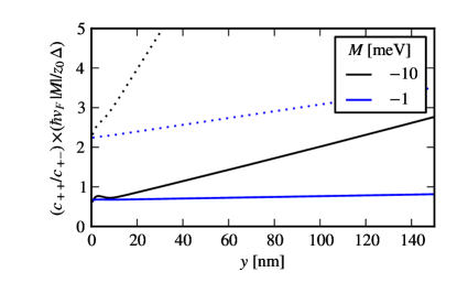
Figure 5: Relative magnitude of the two types of tunneling as a function of location and parameters, at $K=-2k_{F}$ for $P_{++}$ and $K=0$ for $P_{+-}$, as obtained from numerically computed $\hat{\Psi}_{\pm,k}$. The scaling with the electric field is given by $z_{0}\equiv 1\,\mathrm{eV\,nm}\times{}E_{z}/(500\,\nicefrac{\mathrm{mV}}{\mathrm{nm}})$. Solid and dashed lines indicate $\hbar{}v_{F}k_{F}=\pm{}|M|/(6\hbar v_{F})$, i.e., energies $E=E_{\rm Dirac}\mp|M|/6\approx{}(0.75\mp 0.15)|M|$ for the states involved in the $c_{++/+-}$ factors. For $z_{0}/v_{F}\lesssim{}1$, $c_{++}$ is linear in $z_{0}$.

We can now estimate the relative order of magnitude between $P_{++}$ and $P_{+-}$ within this model. From the results above, one can see that the representative quantities to be compared are

$$c_{++}(K,\vec{r}_{1}^{\prime},\vec{r}_{2}^{\prime}) =\frac{\Delta}{i\hbar v_{F}}\partial_{k}P_{++}(\frac{K}{2}+k,\vec{r}_{1}^{\prime};\frac{K}{2}-k,\vec{r}_{2}^{\prime})\rvert_{k=0}\,,$$ (20)

and

$$c_{+-}(K,\vec{r}_{1}^{\prime},\vec{r}_{2}^{\prime}) =P_{+-}(\frac{K}{2}-k_{F},\vec{r}_{1}^{\prime};\frac{K}{2}+k_{F},\vec{r}_{2}^{\prime})\,.$$ (21)

In Fig. 5 we show the ratio of these amplitudes for $\vec{r}_{1}^{\prime}=\vec{r}_{2}^{\prime}=(0,y)$ (i.e., the value at a distance $y$ from the edge). The $c_{++}$ amplitude increases when the energies of the edge states involved approach the TI energy gap edge. The general order of magnitude of the $c_{++/+-}$ factors can be estimated to be of the order

$$c_{++}\sim\frac{\Delta}{|M|}\frac{z_{0}}{\hbar v_{F}}c_{+-}\,.$$ (22)

A similar relation is then expected also between the $\Gamma_{++}$ and $\Gamma_{+-}$ factors for surface contacts to area near $y=0$. Here and below, we characterize the strength of the Rasbha interaction with the quantity $z_{0}\equiv 1\,\mathrm{eV\,nm}\times{}E_{z}/(500\,\nicefrac{\mathrm{mV}}{\mathrm{nm}})$.

Using the above results for the order of magnitude of $c_{++}$ and $c_{+-}$ we find (see Appendix B) the estimates for the general case with $e$-$e$ interactions:

$$\Gamma_{+-} \simeq(a_{0}\Delta)^{\frac{g+g^{-1}}{2}-1}\Gamma_{+-}^{g=1}$$ (23a)

$$\Gamma_{++} \simeq\frac{1}{2}(a_{0}\Delta)^{\frac{g+g^{-1}}{2}-1}\frac{z_{0}\Delta}{v_{F}|M|}\Gamma_{+-}^{g=1}\,,$$ (23b)

corresponding to cutoff $a=\hbar v_{F}/\Delta$. The relation (8) for the noninteracting value $\Gamma_{+-}^{g=1}\simeq(\hbar v_{F}/l_{T})R_{K}/(4R_{N})$ fixes the magnitudes relative to experimental parameters.

With finite electron-electron interactions ($g\neq 1$) in the helical liquid, all the effective tunnel rates obtain identical scaling in the original short-distance cutoff $a_{0}$. This reflects the renormalization of the single-particle tunneling elements $t_{\alpha\sigma}$ by the electron-electron interactions.

We can also estimate the Rashba coupling factor appearing in $\Gamma_{++}$. With a typical TI gap $|M|\sim 10\,\mathrm{meV}\sim 100\,\mathrm{K}$, we see that the factor of $\Delta/|M|$ can be made of the order of $0.1\ldots 0.2$ with conventional superconductors, and can be even larger for smaller TI gaps. The second factor is $z_{0}/\hbar v_{F}\sim E_{z}/(100\,\nicefrac{\mathrm{mV}}{\mathrm{nm}})$, and as visible in Eq. (19), measures the rotation of the spin axis caused by the Rashba mixing. An upper limit for the field that can be applied in practice is likely of the order $E_{z}\sim 100\,\nicefrac{\mathrm{mV}}{\mathrm{nm}}$, as for fields larger than that, the potential difference across the QW becomes comparable to the energy gap of the barrier material (CdTe). Based on this we find an estimate for the achievable ratio, $\Gamma_{++}\sim{}0.1\ldots 1\Gamma_{+-}$.

Finally, let us remark that tunneling that is local in real space, $\langle{\vec{r}}\rvert\hat{h}_{T}\lvert{\vec{r}^{\prime}}\rangle\propto{}\delta(\vec{r}-\vec{r}^{\prime})$, does not lead to tunneling that is local in the edge state Hamiltonian, $t_{\alpha\sigma}(x,\vec{r}^{\prime})\propto\delta(x-x^{\prime})$. This follows in a straightforward way from the extended 2-D nature of the edge states and the $k_{x},k_{y}$ mixing due to the spin-orbit interactions: $\langle{\alpha,x}\rvert\hat{h}_{T}\lvert{\sigma,\vec{r}}\rangle\propto{}\sum_{k}e^{ik(x-x^{\prime})}{\cal Y}_{\alpha,k}(\sigma,y^{\prime},z^{\prime})^{*}$. If the spatial profile ${\cal Y}$ of the wave function has $k$-dependence on the scale $k_{0}$, the sum resembles a rounded $\delta$ function of width $k_{0}^{-1}$. For HgTe QW edge states, $k_{0}^{-1}\sim{}\hbar v_{F}/|M|$ is a low-energy length scale. Because of this, a pointlike contact to a superconductor can produce a finite $P_{++}$, even though assuming $t(x,\vec{r}^{\prime})\propto\delta(x-x^{\prime})$ in Eq. (7) leads to the opposite conclusion.

IV Transport signatures

To study the experimental signatures implied by the above model, we consider the transport problem in the setups depicted in Fig. 1. There, two superconducting contacts are coupled to a helical liquid, whose potential is tuned by additional terminals at the ends. There are three related transport effects one can study here: the equilibrium dc Josephson effect, the ac Josephson effect, and the NS conductance.

We consider a general nonequilibrium case of a time-dependent pair potential $\Delta(t)=|\Delta|e^{i\varphi_{1}(t)}$ in the left contact and $\Delta(t)=|\Delta|e^{i\varphi_{2}(t)}$ in the right one, with $\varphi_{1}(t)=\varphi_{0}/2+2V_{1}t$ and $\varphi_{2}(t)=-\varphi_{0}/2+2V_{2}t$. In Eq. (4), the factors $\Gamma$ inherit this time dependence. We also assume that only sub-gap energies are involved in the transport, so that the quasiparticle current to the superconductors remains exponentially suppressed by the superconducting gap.

The current is obtained as an expectation value of a current operator $\hat{I}=i[H,\hat{N}]$ where $\hat{N}$ is the particle number in the HLL. From the effective Hamiltonian, we identify

$$\hat{I} =\hat{I}_{S1}+\hat{I}_{S2}$$ (24)

$$\hat{I}_{S1} =\sum_{\alpha\beta}\int_{S1}\mathrm{d}x\,2i\Gamma_{\alpha\beta}(x)\psi_{\alpha}(x)\psi_{\beta}(x)+\mathrm{h.c.}\,,$$ (25)

$$\hat{I}_{S2} =\sum_{\alpha\beta}\int_{S2}\mathrm{d}x\,2i\Gamma_{\alpha\beta}(x)\psi_{\alpha}(x)\psi_{\beta}(x)+\mathrm{h.c.}\,,$$ (26)

where $\hat{I}_{S1}$ and $\hat{I}_{S2}$ must be interpreted as the parts corresponding to currents injected through the interfaces at $S1$ and $S2$. The sums over $\alpha\beta$ run over $++$, $+-$, and $--$.

Considering only the Cooperon terms [cf. Fig. 7(a)], using perturbation theory up to second order in $\Gamma$ we find

$$I_{J,S1}(t) =-8\mathop{\mathrm{Im}}\sum_{\alpha\beta}\int_{S1}\mathrm{d}x_{1}\,\int_{S2}\mathrm{d}x_{2}\,X_{\alpha\beta}(x_{1},x_{2})$$ (27)

$$\times e^{i\varphi_{1}(t)}\int_{0}^{\infty}\mathrm{d}t^{\prime}\,e^{-i\varphi_{2}(t-t^{\prime})}\mathop{\mathrm{Im}}[\chi_{\alpha\beta}(x_{1}-x_{2},t^{\prime})]\,,$$

$$I_{J,S2}(t) =I_{J,S1}(t)\rvert_{\varphi_{1}\leftrightarrow\varphi_{2}}\,,$$ (28)

where

$$X_{\alpha\beta}(x_{1},x_{2}) \equiv{}e^{2ik_{F}(\alpha+\beta)(x_{1}-x_{2})}\Gamma_{\alpha\beta}(x_{1})\Gamma_{\alpha\beta}(x_{2})^{*}$$ (29)

$$\chi_{\alpha\beta}(x;t) =\frac{\langle{e^{i\phi_{\alpha}(x,t)}e^{i\phi_{\beta}(x,t)}e^{-i\phi_{\alpha}(0,0)}e^{-i\phi_{\beta}(0,0)}}\rangle_{0}}{(2\pi a)^{2}}\,.$$ (30)

The $\alpha\beta=+-$ component of the current coincides with the result obtained in Ref. Fazio et al., 1995. Note that the terms included here contain the leading order of the dependence in the phase difference $\varphi_{1}-\varphi_{2}$.

The above correlation functions can be evaluated via standard bosonization techniques: Giamarchi (2004)

$$\chi_{\alpha\alpha}(x,t) =(2\pi a)^{-2}B_{\alpha}(x,t)^{g+g^{-1}+2}B_{-\alpha}(x,t)^{g+g^{-1}-2}\,,$$ (31a)

$$\chi_{+-}(x,t) =(2\pi a)^{-2}B_{+}(x,t)^{1/g}B_{-}(x,t)^{1/g}\,,$$ (31b)

$$B_{\pm}(x,t) =\frac{-iaz}{\sinh[z(ut-ia\mp x)]}\,,$$ (31c)

where $z=\pi T/u$.

In the noninteracting case ($g=1$), we can evaluate the time integrals analytically, to order ${\cal O}(a^{3})$:

$$I_{J,S1}(t) =\int_{S1}\mathrm{d}x_{1}\,\int_{S2}\mathrm{d}x_{2}\,[j_{J,S1}^{++}+j_{J,S1}^{--}+j_{J,S1}^{+-}]$$ (32)

$$j_{J,S1}^{++} =\frac{|X_{++}|}{3\pi v_{F}}V_{2}[(V_{2}/\Delta)^{2}+4\pi^{2}(T/\Delta)^{2}]$$ (33)

$$\times\cos\Bigl{(}\varphi_{0}+2V_{1}t-2V_{2}(t-|x_{1}-x_{2}|/v_{F})+\phi_{0}\Bigr{)}\,,$$

$$j_{J,S1}^{--} =0\,,$$ (34)

$$j_{J,S1}^{+-} =-\frac{|X_{+-}|}{\pi v_{F}}\frac{2z}{\sinh(2|x_{1}-x_{2}|z)}$$ (35)

$$\times\sin\Bigl{(}\varphi_{0}+2V_{1}t-2V_{2}(t-|x_{1}-x_{2}|/v_{F})\Bigr{)}\,,$$

where $\phi_{0}(x_{1},x_{2})\equiv{}4k_{F}(x_{1}-x_{2})+\arg[\Gamma_{++}(x_{1})\Gamma_{++}(x_{2})^{*}]$ is a dynamical phase shift.

Below, we discuss the implications of these results first at equilibrium and then at finite biases.

IV.1 Equilibrium

At equilibrium, the leading contribution to the supercurrent comes from the $+-$ channel. As shown in Fig. 6, the supercurrent is finite at zero temperature, and decays exponentially as the temperature is increased above $\hbar v_{F}/d$, in a way that depends on the strength of electron-electron interactions. The qualitative features are the same as those found in Ref. Fazio et al., 1995.

The contribution from the $++$ and $--$ channels to the equilibrium current is not more relevant than $+-$ even in the interacting case, unlike in Ref. Pugnetti et al., 2007. Based on scaling dimensions in the effective Hamiltonian ($\mathrm{dim}\,\psi_{+}\psi_{-}=g^{-1}$, $\mathrm{dim}\,\psi_{+}\psi_{+}=g+g^{-1}$), one finds the scaling $I^{+-}\propto{}(E/\Delta)^{2/g-2}$ and $I^{++/--}\propto{}(E/\Delta)^{2(g+g^{-1})-2}$ for the low-energy scale $E=\max(T,v_{F}/d)$, which implies that $I^{+-}$ will be more relevant than $I^{++/--}$ whatever the interaction parameter. This difference arises from the exclusion principle, which makes the $++/--$ channel less favorable for the supercurrent, although note that with decreasing $g$ (larger repulsive e-e interaction), the ($++/--$) contribution grows relative to the $+-$ one. However, as noted in Section B, the scaling with the bare short-distance cutoff $a_{0}$ as opposed to $\Delta^{-1}$ is identical for $\Gamma_{++/--}$ and $\Gamma_{+-}$.

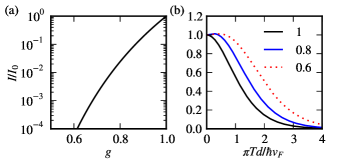
Figure 6: Equilibrium Josephson current between the superconducting contacts, relative to its noninteracting zero-temperature value $I_{0}$. (a) Dependence $\propto{}\Delta^{2-2/g}$ ($T/\Delta=0.1$) on the interaction parameter at $T\ll{}\hbar v_{F}/d$. (b) Temperature dependence for different values of $g$.

IV.2 Nonequilibrium

When the superconductors are biased with a finite voltage, currents generically start to flow between all the terminals, and they may also be time dependent due to the ac Josephson effect. To fully understand these effects, it is illuminating to compute the spatial distribution of the currents in the system.

The spatial dependence of the currents in the helical liquid can be obtained by making use of the following expression for the current operator $\hat{I}=\frac{v_{F}}{\sqrt{\pi}}\partial_{x}\phi(x,t)$ in the Heisenberg picture (see App. C): Virtanen and Recher (2011)

$$\hat{I}(x,t) =\hat{I}_{0}(x,t)+v_{F}\int_{-\infty}^{\infty}\mathrm{d}x^{\prime}\,\mathrm{d}t^{\prime}\,\sum_{\alpha=\pm}\alpha\Bigl{(}$$ (36)

$$\quad\frac{1+g}{2g}D_{\alpha}(x,t;x^{\prime},t^{\prime})-\frac{1-g}{2g}D_{-\alpha}(x,t;x^{\prime},t^{\prime})$$

$$\quad\Bigr{)}\hat{j}_{\alpha}(x^{\prime},t^{\prime})\,,$$

$$\hat{j}_{\alpha}(x^{\prime},t^{\prime}) =\frac{\delta V(t^{\prime})}{\delta\phi_{\alpha}(x^{\prime})}\,.$$ (37)

This applies to any Hamiltonian of the form $H=H_{0}+V(t)$, where $H_{0}$ is the bosonized Hamiltonian in Eq. (1); $\hat{I}_{0}$ is the current operator evolving in time with the unperturbed Hamiltonian $H_{0}$. The operator $j_{\alpha}(x^{\prime},t^{\prime})$ can be interpreted as the current density injected to the mode $\alpha=\pm$ at position $x^{\prime}$ at time $t^{\prime}$. The functions $D_{+(-)}$ are initially right(left)-propagating $\delta$ pulses originating at point $x^{\prime}$ at time $t^{\prime}$.

Let us for simplicity assume that the two superconducting contacts are pointlike in the low-energy model, that $g=1$, and that the helical liquid is homogeneous. Then, $D_{\pm}(x,t;x^{\prime},t^{\prime})=\theta(t-t^{\prime})\delta(x-x^{\prime}\mp v_{F}(t-t^{\prime}))$ and we find

$$I(x,t) =\sum_{j=1,2}\bigl{[}\theta(x-x_{j})l_{T}\langle{\hat{I}_{+,j}(t-\frac{|x-x_{j}|}{v_{F}})}\rangle$$ (38)

$$\qquad-\theta(x_{j}-x)l_{T}\langle{\hat{I}_{-,j}(t-\frac{|x-x_{j}|}{v_{F}})}\rangle\bigr{]}\,.$$

$$\hat{I}_{+,j} =\frac{\partial}{\partial\phi_{+}}\Bigl{[}\Gamma_{++}\psi_{+}\psi_{+}+\Gamma_{--}\psi_{-}\psi_{-}$$

$$\qquad+\Gamma_{+-}\psi_{+}\psi_{-}+\mathrm{h.c.}\Bigr{]}\rvert_{x=x_{j}}$$ (39)

$$=2i\Gamma_{++}\psi_{+}\psi_{+}+i\Gamma_{+-}\psi_{+}\psi_{-}+\mathrm{h.c.}\,,$$

$$\hat{I}_{-,j} =2i\Gamma_{--}\psi_{-}\psi_{-}+i\Gamma_{+-}\psi_{+}\psi_{-}+\mathrm{h.c.}\,,$$ (40)

where $l_{T}$ is the small contact size, and the expectation values $\langle{\cdot}\rangle$ closely correspond to the different parts of the injection currents $I_{J,S1/S2}$ evaluated in the previous section. Indeed,

$$\langle{\hat{I}_{+,1}(t)}\rangle =j^{++}_{S1}(t)+\frac{1}{2}j^{+-}_{S1}(t)\,,$$ (41a)

$$\langle{\hat{I}_{-,1}(t)}\rangle =j^{--}_{S1}(t)+\frac{1}{2}j^{+-}_{S1}(t)\,,$$ (41b)

$$\langle{\hat{I}_{+,2}(t)}\rangle =j^{++}_{S2}(t)+\frac{1}{2}j^{+-}_{S2}(t)\,,$$ (41c)

$$\langle{\hat{I}_{-,2}(t)}\rangle =j^{--}_{S2}(t)+\frac{1}{2}j^{+-}_{S2}(t)\,.$$ (41d)

The physical interpretation is particularly simple: the contacts at $x_{1}$ and $x_{2}$ inject current to the helical liquid. The component due to $+-$ tunneling splits evenly to the left and right-moving modes, whereas the $++$ and $--$ components end up solely in the $+$ and $-$ modes, respectively. Within each edge mode, the injected current propagates with the Fermi velocity, as indicated by the retarded time arguments.

The calculations done in the previous section indicated that in this case $j_{S1}^{--}=0$ and $j^{++}_{S2}=0$ to leading order in $a$. Therefore, essentially all of the current injected by the $++$ and $--$ tunneling in fact flows only to the reservoirs that maintain the chemical potential of the helical liquid at $\mu=0$, rather than between the two superconducting contacts, which can be verified by computing the current at $x<x_{1},x_{2}$ and at $x>x_{1},x_{2}$. The effect essentially amounts to a modulation of the NS conductance between the superconductors and the normal leads by the (time-dependent) phase difference $\varphi_{1}(t)-\varphi_{2}(t)$ between the superconducting contacts.

Based on the above results, we can write down an expression for the part of the NS current [see Fig. 1(c)] that depends on the phase difference, in the configuration $V_{1}=V_{2}=V$:

$$\delta I_{NS} =\frac{2l_{T}^{2}|X_{++}|}{3\pi}V\cos(2Vd+\phi_{0})\cos(\varphi_{0})$$ (42)

$$\qquad\times[(V/\Delta)^{2}+4\pi^{2}(T/\Delta)^{2}]$$

$$+\frac{4l_{T}^{2}|X_{+-}|}{\pi}\sin(2Vd)\cos(\varphi_{0})\frac{z}{\sinh(2zd)}\,.$$

Note that the modulation of the NS conductance from the $+-$ channel decays exponentially as the temperature increases, whereas the $++$ contribution does not. The same situation should persist in all orders of perturbation in the effective Hamiltonian for the $+-$ tunneling: the terms coupling to $\varphi_{0}$ contain inequal numbers of $\psi_{+}(d)\psi_{-}(d)$ and $\psi_{+}^{\dagger}(d)\psi_{-}^{\dagger}(d)$, which implies that the correlation function is of the form $[B_{+}(d,t)B_{-}(d,t)]\times{\cal O}(1)$ and thus has an overall exponential prefactor $e^{-2\pi Td/v_{F}}$. Therefore, there in principle is a temperature regime at $T\gg{}\hbar v_{F}/k_{B}d$ in which the leading contribution to the $\varphi_{0}$ dependence of the NS current comes mainly from the $++$ tunneling, despite the power-law suppression of this channel in helical liquids. The physical reason for the difference can be seen in Fig. 2: for the $+-$ channel an electron pair injected to energies $\pm\varepsilon$ and traversing through the junction obtains an energy dependent phase factor $e^{i(k_{1}+k_{2})d}=e^{-2i\varepsilon{}d/v_{F}}$, typical of Andreev reflection, which averages towards zero when a finite energy window is considered. For the $++$ channel, because of the linear spectrum, the corresponding phase factor $e^{2ik_{F}d}$ is energy-independent and no such averaging occurs.

The above result requires validity of the perturbation theory, i.e., $l_{T}\Gamma_{+-}\sim{}R_{K}/4R_{N}\lesssim{}1$ where $l_{T}$ is the contact length. If this condition is not satisfied, an additional contribution decaying only as $1/T$ in temperature arises in the $+-$ channel. This additional proximity effect contribution is similar to what occurs in metallic systems of a more macroscopic size, Pothier et al. (1994); *hekking1993-iot; *volkov1997-lpe although there it can be much amplified as the electrons can stay a long time near the NS interface due to impurity scattering.

With finite repulsive interactions ($g<1$), also the $+-$ contribution to the NS conductance obtains a power-law prefactor according to the scaling dimensions, $I^{+-}\propto{}(E/\Delta)^{2/g-2}$ with $E=\max(T,V)$, and the prefactor of the $++$ part is modified, $I^{++/--}\propto{}(E/\Delta)^{2(g+g^{-1})-2}$. According to the correlation functions (31), exponential decay will also appear in the $++$ part due to charge fractionalization, but it will be weaker than in the $+-$ part for all values of $g$.

A second distinguishing feature of the $++$ contribution to the NS current is that it is expected to oscillate not only as a function of the bias, but also as a function of the Fermi wave vector appearing in the dynamical phase $\phi_{0}$. In metals or other systems where $k_{F}$ is large, the wavelength of such oscillations would be on the atomic length scales, and the contribution would average to zero [as $\sim\mathop{\mathrm{sinc}}(k_{F}w)^{2}$] over any practical contact size $w$. Pugnetti et al. (2007) However, this needs not be the case in HgTe-QW (or in nanotubes, see Ref. Pugnetti et al., 2007) when the Fermi level lies close to the Dirac point: for example assuming $|\mu-E_{\rm Dirac}|\sim{}M/6\sim 1.5\,\mathrm{meV}$ one finds $1/k_{F}\sim 150\,\mathrm{nm}$. Such length scales are likely experimentally accessible.

One should also note that the finite wave velocity combined with the ac Josephson effect causes some additional effects. The current propagates at the (renormalized) Fermi velocity $v_{F}/g$, rather than at the substantially higher speed of light $c$ at which electromagnetic excitations propagate. Assuming only the $+-$ channel contributes, one can find the spatial dependence of current between the two contacts:

$$I(t) \propto\sin[2Vt-\frac{2Vx}{v_{F}}]+\sin[2Vt-\frac{2V(d-x)}{v_{F}}]\,.$$ (43)

Based on this, it is clear that for biases $V\gtrsim\hbar v_{F}/ed$ between the two superconducting electrodes, the ac Josephson effect must be associated with appreciable standing wave oscillations in the charge density. This behavior is not specific to helical liquids: a similar spatially resolved calculation as above for the spinful liquid ac Josephson effect of Ref. Fazio et al., 1995 should also produce this feature. Whether such effects are observable in reality, however, depends on how realistic the model assumptions about screening are in the systems studied (see also Ref. Egger and Grabert, 1998).

V Discussion and conclusions

In this work we considered the proximity effect induced in a helical edge state, taking into account a spatially and energetically non-constant spin quantization axis. Such rotation of the spin axis naturally arises from the spin-orbit interaction in real materials such as the HgTe QWs, for example in a controlled way by structure inversion symmetry breaking Rashba terms. This has the consequence that the singlet correlations in an s-wave superconductor can also induce a proximity effect in the same channel of left and right-movers ($\Gamma_{++/--}$) in addition to the usual term where the correlation is between opposite chiral states (with amplitude $\Gamma_{+-}$). We derived a description of the proximity effect in both channels in the presence of Rashba interaction using a simple model for the tunneling between the superconductor and the helical edge state, respecting spin conservation and time reversal symmetries.

The extra transport channels ($++/--$) describe processes that are in principle parasitic for the splitting of a Cooper pair into two electrons propagating into different directions (the $+-$ channel) Sato et al. (2010). For a single superconducting contact to the helical liquid, the scaling with temperature (or bias voltage) at low energies however always favors the $+-$ channel. In Ref. Recher and Loss, 2002, the two-particle tunneling into the bulk of a spinful Luttinger liquid was found to be suppressed in a power law in $1/\Delta$ similarly as here, but there the tunneling into the $++/--$ channel was found to be dominant. The difference arises because in a spinful liquid the two opposite spins can tunnel into different spin channels, and therefore no Pauli-blocking factors appear.

Observing effects related to the same-mode tunneling ($\Gamma_{++}$) is likely rather challenging, as they can be suppressed relative to $\Gamma_{+-}$ by several factors: the power law suppression $(T/\Delta)^{2}+(V/\Delta)^{2}$ from exclusion principle, suppression of the tunneling factor $\Gamma_{++}$ itself, and averaging effects related to contacts if they are larger than $1/k_{F}$ (i.e. $\sim 150\,\mathrm{nm}$ for parameters in Fig. 5). However, by observing the dependence of the NS conductance on the superconducting phase, the relative difference can be reduced due to the exponential dephasing of the $+-$ contribution at high temperatures. (In the case that the only mode of transport is via the $+-$ channel, the modulation would still contain features distinct to ballistic transport, such as oscillations as the bias voltage is increased.) The question is therefore more on how small signals can be detected in the conductance, oscillating with the phase difference $\varphi_{0}$, and how large the thermal factor $2\pi k_{B}Td/\hbar v_{F}$ can be made before inelastic interaction effects (e.g. electron-phonon scattering), which we have neglected, start to play a role.

We find that controlling the spin axis via external electric fields in HgTe-QW in general requires very strong fields, because of the weak coupling of the additional spin-orbit interactions to the edge states. For our case, this makes achieving a large $\Gamma_{++}$ more difficult, and may in general pose problems to proposals relying on the control of the spin axis. Making an optimistic estimate, we find from Eqs. (23) and (42) that the ratio of the two contributions to the amplitude of phase-dependent oscillations in the conductance is ($V\ll{}T$, $g=1$, $E_{z}\sim{}100\,\nicefrac{\mathrm{mV}}{\mathrm{nm}}$)

$$\frac{\delta G_{++}(\varphi_{0})}{\delta G_{+-}(\varphi_{0})} =\frac{2\pi^{2}}{3}\left|\frac{\Gamma_{++}}{\Gamma_{+-}}\right|^{2}\left(\frac{k_{B}T}{\Delta}\right)^{2}\mathop{\mathrm{sinhc}}\left(\frac{2\pi k_{B}Td}{\hbar v_{F}}\right)$$ (44)

$$\sim\left(\frac{k_{B}T}{M}\right)^{2}\mathop{\mathrm{sinhc}}(2\pi k_{B}Td/\hbar v_{F})\,,$$

where $\mathop{\mathrm{sinhc}}(x)=\sinh(x)/x$. With finite $e$-$e$ interactions [cf. Eq. (78)], the ratio is multiplied by $(\Delta/T)^{2-2g}$, making the result depend only on $\Delta/M$ in the limit $g\to 0$, and the exponential dependence becomes $\sim\exp(2\pi g[2-g]k_{B}Td/\hbar v_{F})$. Taking junction length $d=3\,\mathrm{\mu m}$, the temperature scale of the exponential suppression factor is $E_{T}\equiv\hbar v_{F}/(2\pi d)\approx 0.2\,\mathrm{K}$, and the ratio becomes unity at the cross-over temperature $T_{*}\approx E_{T}\{\log[2(M/E_{T})^{2}]-\log\log[2(M/E_{T})^{2}]\}\approx{}2.2\,\mathrm{K}$, which depends weakly on $M$ (here $M=-10\,\mathrm{meV}$). Given a suitable superconducting material, this should be achievable.

Another option for amplifying the same-mode tunneling could be to break the time-reversal symmetry and introduce additional spin flips or spin rotation, for example via magnetic impurities or ferromagnets. The effect could still be detected in the NS conductance, as that conclusion is only based on the generic form of the low-energy effective Hamiltonian.

Observe that in our analysis the true 2D nature of the edge states in HgTe-based QWs was important. The ($++/--$) proximity channel cannot be found in a completely 1D description, as in such a picture the spin quantization axis is simply rotated globally by the Rashba terms (cf. Refs. Sato et al., 2010; Väyrynen and Ojanen, 2011). Such rotations can have no consequences for Cooper pair injection into a single edge, due to the $s$-wave symmetry of the pairing [cf. Eq. (9)]. Spatially inhomogeneous Rashba interaction, Ström et al. (2010) could, however, induce a finite $++/--$ amplitude.

As in other systems with small critical currents, Fazio et al. (1995) also here thermal fluctuations in the superconducting phase difference are a problem for measurements of the temperature-dependence of the Josephson effect: the temperature scale relevant for the phase fluctuations, $E_{J}=\hbar I_{c}/2e$, is smaller than the intrinsic one, $E_{T}=\hbar v_{F}/d$. More complicated measurement schemes Golubov et al. (2004); Della Rocca et al. (2007) than the simple current-biased setup in Fig. 1(b) may nevertheless help in overcoming this problem. One should, however, note that only the Josephson current is a problematic observable in this respect. The measurement of phase oscillations of the NS conductance in the setup of Fig. 1(c) is expected to suffer much less from phase fluctuations, as there the phase difference is locked by the magnetic flux and the large critical current of the superconducting loop itself.

In summary, starting from a tunneling Hamiltonian, we derived an effective low-energy theory describing the superconducting proximity effect in the helical edge state of a 2D topological insulator. We showed that in these systems, despite the s-wave symmetry of the superconductor, correlations can occur both in ($++/--$) and between ($+-$) the left and right moving modes, and within a simple model, we estimated the expected magnitudes for the effective proximity gap parameters in HgTe/CdTe quantum wells. Based on the effective Hamiltonian, we studied the dc and ac Josephson effects in the helical liquid, and considered phase-dependent oscillations of the NS conductance. In nonequilibrium, we found that correlations within the same mode can give rise to a long-ranged interference effect, which could act as a signature of their presence. Our results also shed light on the meaning of ”spin” in the helicity of these edge states which is of importance if one intends to use these edge states for spin-injection or spin-detection.

Appendix A HgTe/CdTe QW edge states

The edge states of a HgTe-QW can be described within the four-band model introduced in Ref. Bernevig et al., 2006. Here, we derive explicit analytical expressions for the edge states in a single edge following the approach of Ref. Zhou et al., 2008, for use in Section. III.2, and to demonstrate that the direction where the 4-band spinors point is independent of $k$ and $M$, in the absence of inversion symmetry breaking terms.

The four-band Hamiltonian reads

$$H =\begin{pmatrix}h(k)&0\\ 0&h(-k)^{*}\end{pmatrix}\,,$$ (45)

$$h(k) =\epsilon(k)\sigma_{0}+\vec{d}(k)\cdot\vec{\sigma}\,,\;\epsilon(k)=C-D|\vec{k}|^{2}\,,$$ (46)

$$\vec{d}(k) =(Ak,-Ak_{y},M-Bk^{2})\,.$$ (47)

For the parameters $A$, $B$, $C$, $D$ we use values from Ref. Rothe et al., 2010: $A=365\,\mathrm{meV\,nm}$, $B=-706\,\mathrm{meV\,nm^{2}}$, $D=-532\,\mathrm{meV\,nm^{2}}$ and take $C=0$ (it only shifts the Dirac point). For an edge with QW lying at $y>0$, with the wave function vanishing at $y=0$, the edge eigenstates are:

$$\hat{\Psi}_{+,k} =\begin{pmatrix}\hat{\Phi}_{+,k}\\ 0\end{pmatrix}\,,\;\hat{\Psi}_{-,k}=\begin{pmatrix}0\\ \hat{\Phi}_{-,k}\end{pmatrix}\,,$$ (48)

$$\hat{\Phi}_{\alpha,k} =Ne^{-ikx}\bigl{[}e^{-\lambda_{1}y}-e^{-\lambda_{2}y}\bigr{]}\begin{pmatrix}-\sqrt{D-B}\\ \sqrt{-D-B}\end{pmatrix}\,,$$ (49)

where

$$E =\frac{-DM}{B}-\alpha k\frac{A\sqrt{B^{2}-D^{2}}}{B}\,,$$ (50)

$$\lambda_{1/2} =\sqrt{k^{2}+F\mp\sqrt{F^{2}-Q^{2}}}\,,$$ (51)

$$F =\frac{A^{2}-2(BM+DE)}{2(B^{2}-D^{2})}\,,\;Q^{2}=\frac{M^{2}-E^{2}}{B^{2}-D^{2}}\,,$$ (52)

and $N$ is a normalization constant.

Note that the spinor points to a single direction independent of $k$ or energy $E$, so that the above results are of the form

$$\hat{\Psi}_{+,k}=\begin{pmatrix}\hat{\chi}\\ 0\end{pmatrix}f_{+,k}\,,\;\hat{\Psi}_{-,k}=\begin{pmatrix}0\\ \hat{\chi}\end{pmatrix}f_{-,k}\,,$$ (53)

where the constant spinor $\hat{\chi}$ is normalized ($\hat{\chi}^{\dagger}\hat{\chi}=1$) and depends only on the parameters $B$ and $D$. The envelope $f_{\alpha,k}(x,y)=N^{\prime}e^{ikx}[e^{-\lambda_{1}y}-e^{-\lambda_{2}y}]$ is a scalar function. Using the above parameters we find $\hat{\chi}=(0.35,0.94)^{T}$, so that the spinor has the main contribution in the $H1$ band.

Appendix B Low-energy Hamiltonian

Figure 7: (a) Cooperon giving a contribution to the Josephson current. (b) Integrating out the relative coordinates gives an effective description of Andreev reflection.

In this Appendix, we derive the effective Hamiltonian in Eq. (4) via perturbative renormalization group (RG), Giamarchi (2004) aiming to approximate the Cooperon term [see Fig. 7(a)] appearing in the perturbation expansion in the tunneling with the effective term in Fig. 7(b). When computing the Josephson current, for the $\Gamma_{+-}$ channel this approach is compatible with that used in Ref. Fazio et al., 1995 and elsewhere in the long-junction case. For the $\Gamma_{++}$ and $\Gamma_{--}$ channels we however need to pay more attention to the tunneling elements.

We take our effective Hamiltonian to have the form:

$$H_{\rm eff} =H_{0}+H_{T}+H_{T2}=H_{0}+V\,,$$ (54)

$$H_{T} =\sum_{\alpha=\pm,\sigma^{\prime}=\uparrow,\downarrow}\int\mathrm{d}x\,\mathrm{d}^{3}r^{\prime}\,t_{\alpha\sigma^{\prime}}(x,\vec{r}^{\prime})\psi^{\dagger}_{\alpha}(x)\psi_{S\sigma^{\prime}}(\vec{r}^{\prime})+\mathrm{h.c.}$$ (55)

$$H_{T2} =\sum_{\alpha\beta}\int\mathrm{d}x\,\Gamma_{\alpha\beta}(x)\psi_{\alpha}(x)\psi_{\beta}(x+a)+\mathrm{h.c.}\,,$$ (56)

and rescale only the cutoff in the helical liquid in the progress of RG. Because correlations in the superconductor decay exponentially at distances $\gtrsim\Delta^{-1}$, and because the superconducting gap prohibits dissipation at low energies inside the superconductor, $H_{T}$ can be neglected in calculations after the scaling to low-energy length scales $\gg{}\Delta^{-1}$ is done — which reduces the effective Hamiltonian to that in Eq. (4).

The scaling equations read

$$\frac{\mathrm{d}t_{\alpha\sigma^{\prime}}\,}{\mathrm{d}l\,} =[2-\eta_{1}]t_{\alpha\sigma^{\prime}}$$ (57)

$$\frac{\mathrm{d}\Gamma_{\alpha\beta}\,}{\mathrm{d}l\,} =[2-\eta_{2,\alpha\beta}]\Gamma_{\alpha\beta}+S_{\alpha\beta}(l)\,,$$ (58)

where $\eta_{1}=(g+g^{-1})/4$ is the scaling dimension of $e^{i\phi_{\pm}}$ appearing in tunneling $H_{T}$, and $\eta_{2,\alpha,-\alpha}=1/g$ and $\eta_{2,\alpha,\alpha}=g+g^{-1}$ are scaling dimensions of the operators in $H_{T2}$. Although essentially a standard calculation, below we explain the derivation of $S_{\alpha\beta}$ in detail.

Below, we need the factorization

$$\psi_{\alpha_{1}}(x_{1},\tau_{1})\psi_{\alpha_{2}}(x_{2},\tau_{2})=(a_{0}q_{0})^{2\eta_{1}}\frac{U_{\alpha_{1}}(\tau_{1})U_{\alpha_{2}}(\tau_{2})}{2\pi a_{0}}$$ (59)

$$\times e^{ik_{F}(\alpha_{1}x_{1}+\alpha_{2}x_{2})}$$

$$\times{:e^{i\phi_{\alpha_{1}}(x_{1},\tau_{1})}e^{i\phi_{\alpha_{2}}(x_{2},\tau_{2})}:}\,C_{\alpha_{1},\alpha_{2}}(x_{1}-x_{2},\tau_{1}-\tau_{2})\,,$$

where $q_{0}=2\pi/L$ is the infrared cutoff, and the correlation functions read

$$C_{++}(z) =(q_{0}z)^{g^{-1}(\frac{1+g}{2})^{2}}(q_{0}z^{*})^{g^{-1}(\frac{1-g}{2})^{2}}$$ (60)

$$C_{\alpha,-\alpha}(z) =|q_{0}z|^{(1-g^{2})/(2g)}\,,$$ (61)

where $C_{\alpha\beta}(x,\tau)=C_{\alpha\beta}(z)$, $z=v_{F}\tau-ix$, and $C_{--}(z)=C_{++}(z)^{*}$. Observe that $C_{\alpha_{1}\alpha_{2}}(z)\propto q_{0}^{\eta_{2,\alpha_{1}\alpha_{2}}-2\eta_{1}}$.

To perform the RG steps, we also need the corresponding operator product expansions. Taking sign changes due to Klein factors and time ordering into account, we find [cf. Eq. (59)]:

$$T[\psi_{\alpha_{1}}(z_{1})\psi_{\alpha_{2}}(z_{2})]$$ (62)

$$\simeq u_{\alpha_{1}\alpha_{2}}(z_{1}-z_{2})\psi_{\alpha_{1}}(\frac{z_{1}+z_{2}}{2})\psi_{\alpha_{2}}(\frac{z_{1}+z_{2}}{2}+a_{0})\,,$$

where

$$u_{\alpha_{1}\alpha_{2}}(z)=e^{i(\alpha_{1}-\alpha_{2})k_{F}x/2}\mathop{\mathrm{sgn}}(\tau)^{\delta_{\alpha_{1},\alpha_{2}}}$$ (63)

$$\times\frac{C_{\alpha_{1},\alpha_{2}}(x\mathop{\mathrm{sgn}}(\tau),|\tau|)}{C_{\alpha_{1},\alpha_{2}}(0,a_{0})}\,,$$

and $\delta_{\alpha_{1},\alpha_{2}}$ in the sign factor arises from the fact that $U_{\alpha_{1}}U_{\alpha_{2}}=(-1)^{1+\delta_{\alpha_{1},\alpha_{2}}}U_{\alpha_{2}}U_{\alpha_{1}}$.

The source term $S_{\alpha\beta}(l)$ for the Andreev reflection processes $\Gamma_{\alpha\beta}$ appears from the second-order term in the pertubation expansion of the partition function, $Z/Z_{0}=\langle{Te^{-\int_{0}^{\beta}\mathrm{d}\tau\,\lambda V(\tau)}}\rangle_{0}=1+c_{1}\lambda+c_{2}\lambda^{2}+\ldots$. Combining two $H_{T}$ and using the operator product expansions gives a contribution to $\Gamma_{\alpha\beta}$. We also trace out the superconductors at this step, factorizing the expectation value to $\langle{\ldots}\rangle_{0}=\langle{\ldots}\rangle_{HLL,0}\langle{\ldots}\rangle_{S,0}$. This yields the result

$$\frac{\mathrm{d}c_{2}\,}{\mathrm{d}l\,} =\int\mathrm{d}^{2}z\,\sum_{\alpha\beta}\langle{T[\psi_{\alpha}(z)\psi_{\beta}(z+a_{0})]}\rangle_{0}S_{\alpha\beta}(l,z)\,,$$ (64)

$$S_{\alpha\beta}(l,z) =a_{0}[\partial_{r}f_{\alpha\beta}(l,z,r)]_{r=a_{0}}\,,$$ (65)

$$f_{\alpha\beta}(l,z,r) =\int_{|z^{\prime}|<r}\mathrm{d}^{2}z^{\prime}\,c_{\alpha\beta}(l,z,z^{\prime})\,,$$ (66)

$$c_{\alpha\beta}(l,z,z^{\prime}) =\frac{1}{2}\int\mathrm{d}^{3}r_{1}^{\prime}\,\mathrm{d}^{3}r_{2}^{\prime}\,\sum_{\sigma_{1}\sigma_{2}=\uparrow,\downarrow}$$ (67)

$$\times t_{\alpha\sigma_{1}}(x+x^{\prime}/2,\vec{r}_{1}^{\prime})^{*}t_{\beta\sigma_{2}}(x-x^{\prime}/2,\vec{r}_{2}^{\prime})^{*}$$

$$\times F^{\dagger}(\sigma_{1},\vec{r}_{1}^{\prime},\tau^{\prime};\sigma_{2},\vec{r}_{2}^{\prime},0)u_{\alpha\beta}(l,z^{\prime})\,,$$

where $\mathrm{d}^{2}z\,$ is shorthand for $\mathrm{d}x\,\mathrm{d}\tau\,$. This closes the set of equations.

We can now solve the scaling equations:

$$t_{\alpha\sigma^{\prime}}(l) =e^{(2-\eta_{1})l}t_{\alpha\sigma}(0)\,,$$ (68)

$$\Gamma_{\alpha\beta}(l,z) =\int_{0}^{l}\mathrm{d}s\,e^{(2-\eta_{2,\alpha\beta})(l-s)}S_{\alpha\beta}(s,e^{l-s}z)\,.$$ (69)

The integral appearing in $\Gamma_{\alpha\beta}$ can be simplified by substituting in the scaling obtained for $t_{\alpha\beta}$, and undoing the rescaling of length scales in the remaining integrals. This yields:

$$u_{\alpha\beta}(l,z) =e^{[2\eta_{1}-\eta_{2,\alpha\beta}]l}u_{\alpha\beta}(0,e^{l}z)$$ (70)

$$c_{\alpha\beta}(l,z,z^{\prime}) =e^{[4-\eta_{2,\alpha\beta}]l}c_{\alpha\beta}(0,e^{l}z,e^{l}z^{\prime})$$ (71)

$$f_{\alpha\beta}(l,z,r) =e^{[2-\eta_{2,\alpha\beta}]l}f_{\alpha\beta}(0,e^{l}z,e^{l}r)\,,$$ (72)

$$S_{\alpha\beta}(l,z) =e^{[3-\eta_{2,\alpha,\beta}]l}a_{0}[\partial_{r}f_{\alpha\beta}(0,e^{l}z,r)]_{r=a_{0}e^{l}}$$ (73)

And further,

$$\Gamma_{\alpha\beta}(l,z) =e^{[2-\eta_{2,\alpha\beta}]l}\int_{a_{0}<|z^{\prime}|<a(l)}\mathrm{d}^{2}z^{\prime}\,c_{\alpha\beta}(0,e^{l}z,z^{\prime})\,,$$ (74)

where $a(l)=a_{0}e^{l}$. Here, $c_{\alpha\beta}$ decays fast for $|z^{\prime}|>|\Delta|^{-1}$ due to the decaying $F$ functions and the assumedly short range of tunneling. Therefore, at long length scales $a=a_{0}e^{l}\gg{}|\Delta|^{-1}$ we can replace the upper limit in the integral: $a\mapsto{}\infty$.

Undoing all length rescaling, we can write the result in the form of Eq. (4), with

$$\Gamma_{\alpha\beta}(x) =\frac{1}{4}\int\mathrm{d}^{3}r_{1}^{\prime}\,\mathrm{d}^{3}r_{2}^{\prime}\,\mathrm{d}x\,^{\prime}\mathrm{d}\tau\,^{\prime}e^{i(\alpha-\beta)k_{F}x^{\prime}/2}$$ (75)

$$\times P_{\alpha\beta}(x+\frac{x^{\prime}}{2},\vec{r}_{1}^{\prime};x-\frac{x^{\prime}}{2},\vec{r}_{2}^{\prime})^{*}F^{\dagger}(\vec{r}_{1}^{\prime},\tau^{\prime};\vec{r}_{2}^{\prime},0)$$

$$\times\frac{a^{1-\eta_{2,\alpha\beta}}C_{\alpha\beta}(x^{\prime}\mathop{\mathrm{sgn}}(\tau^{\prime}),|\tau^{\prime}|)\mathop{\mathrm{sgn}}(\tau^{\prime})^{\delta_{\alpha\beta}}}{a_{0}^{1-\eta_{2,\alpha\beta}}C_{\alpha\beta}(0,a_{0})}\,,$$

where

$$P_{\alpha_{1}\alpha_{2}}(x_{1},\vec{r}_{1}^{\prime};x_{2},\vec{r}_{2}^{\prime}) \equiv[t_{\alpha_{1}\downarrow}(x_{1},\vec{r}_{1}^{\prime})t_{\alpha_{2}\uparrow}(x_{2},\vec{r}_{2}^{\prime})$$ (76)

$$-t_{\alpha_{1}\uparrow}(x_{1},\vec{r}_{1}^{\prime})t_{\alpha_{2}\downarrow}(x_{2},\vec{r}_{2}^{\prime})]+[\vec{r}_{1}^{\prime}\leftrightarrow{}\vec{r}_{2}^{\prime}]\,,$$

and we have made use of the singlet symmetry of the $F$ function. The cutoff $a$ in the theory specified by Eqs. (4) and (75) can be chosen freely, but taking $a=|\Delta|^{-1}$ is natural as the source term in the original RG stops contributing at that length scale.

Consider the noninteracting case, $g=1$. There,

$$\frac{a^{1-\eta_{2,\alpha\beta}}C_{\alpha\beta}(x\mathop{\mathrm{sgn}}(\tau),|\tau|)\mathop{\mathrm{sgn}}(\tau)^{\delta_{\alpha\beta}}}{a_{0}^{1-\eta_{2,\alpha\beta}}C_{\alpha\beta}(0,a_{0})}=\begin{cases}a^{-1}[v_{F}\tau-ix]\,,\\ 1\,,\end{cases}$$ (77)

for $\alpha\beta=++$ and $\alpha\beta=+-$, respectively. One also notes that $\Gamma_{-+}\psi_{-}\psi_{+}=-\Gamma_{+-}\psi_{-}\psi_{+}=\Gamma_{+-}\psi_{+}\psi_{-}$, so we redefine $\Gamma_{+-}\mapsto{}2\Gamma_{+-}$ as the sum of the two and drop the $-+$ term. Finally, going into Fourier representation yields Eqs. (5) and (6). Due to the integrals over $x^{\prime}$ and $\tau^{\prime}$ extending over the whole range, and the correlation functions $C_{\alpha\beta}$ being local in frequency and energy, only certain energies and momenta contribute in the final result.

To find out the effect of interactions, one needs to roughly estimate the result from Eq. (75). First, since $k_{F,S}^{-1}$ in the superconductor is a short length scale, we take $F(\vec{r}_{1}^{\prime},\tau^{\prime};\vec{r}_{2}^{\prime},0)\mapsto F(\tau^{\prime})\delta(\vec{r}_{1}^{\prime}-\vec{r}_{2}^{\prime})$, $F(\tau^{\prime})=N_{F}\Delta K_{0}(|\tau|\Delta)$, where $N_{F}$ is the normal-state DOS at Fermi energy in the superconductor, and $|\tau|T\ll 1$, $T\ll\Delta\ll|M|$. We consider tunneling that is local on length scales of $1/\Delta$ (and $1/T$ and the other low-energy scales) and replace $P_{+-}\sim{\cal K}\delta(x^{\prime})\delta(x-x_{1}^{\prime})$ with ${\cal K}$ a constant. Based on the model in Sec. (III.2), the Fourier transform of $P_{++}$ in $x^{\prime}$ satisfies $P_{++}\sim-ik(z_{0}/M)P_{+-}$ on long wavelengths $|k|\ll{}M$, with $P_{+-}$ constant in $k$. In real space we then have $P_{++}\sim{\cal K}\frac{z_{0}}{M}\partial_{x^{\prime}}\delta(x^{\prime})\delta(x-x_{1}^{\prime})$. Within these assumptions, we get

$$\Gamma_{+-} \sim{\cal K}N_{F}a^{1-\eta_{2}}a_{0}^{2\eta_{1}-1}\Delta\int_{0}^{\infty}\mathrm{d}\tau^{\prime}\,K_{0}(\Delta|\tau^{\prime}|)C_{+-}(\frac{v_{F}\tau^{\prime}}{q_{0}})$$ (78a)

$$={\cal K}N_{F}(a\Delta)^{1-1/g}(a_{0}\Delta)^{\frac{g+g^{-1}}{2}-1}q(\frac{g^{-1}-g}{2})\,,$$ (78b)

$$\Gamma_{++} \sim{\cal K}N_{F}\frac{a^{1-\eta_{2}}a_{0}^{2\eta_{1}-1}\Delta z_{0}}{2|M|}\int_{0}^{\infty}\mathrm{d}\tau^{\prime}\,K_{0}(\Delta|\tau^{\prime}|)$$ (78c)

$$\qquad\times i\partial_{x^{\prime}}\mathop{\mathrm{Im}}C_{++}(\frac{v_{F}\tau^{\prime}-ix^{\prime}}{q_{0}})\rvert_{x^{\prime}=0}$$

$$=\frac{i{\cal K}N_{F}}{2}(a\Delta)^{1-g-1/g}(a_{0}\Delta)^{\frac{g+g^{-1}}{2}-1}\frac{z_{0}\Delta}{v_{F}|M|}$$ (78d)

$$\qquad\times q(\frac{g^{-1}+g}{2}-1)\,,$$

where $q(x)=2^{x-1}\Gamma(\frac{1+x}{2})^{2}\sim 1$. The effective tunnel rates obtain an identical scaling in the bare short-distance cutoff $a_{0}$ related to interactions, which appears because of a renormalization of the tunneling elements $t_{\alpha\sigma}$. The low-energy scaling with $a$ follows the scaling dimensions in the effective Hamiltonian. Finally, $\Gamma_{++}$ has an additional factor $z_{0}\Delta/v_{F}|M|$ that is a signature of the Rashba coupling.

The expression (5) for $\Gamma_{++}$ deserves some comments: First, we know that $F(\omega)\simeq{}1+c\omega^{2}$ for $\omega\to 0$, so that $\partial_{\omega}F\rvert_{\omega=0}$ vanishes, and from Eq. (11) we know that $P_{++}(-k)=-P_{++}(k)$ which means that $\partial_{k}P_{++}$ is even in $k$ and can be finite at $k=0$. Note that the gradients $\partial_{\omega}$, $\partial_{k}$ appear because the boson correlation function $\langle{e^{i\phi_{+}(x,\tau)}e^{i\phi_{+}(0,0)}}\rangle_{0}$ vanishes at $x,\tau\to 0$ [see Eq. (77)], which reflects the fermionic exclusion principle. This is the reason why the effective Hamiltonian contains a term resembling more $\psi_{+}\psi_{+}$ than $\psi_{+}k\psi_{+}$, which is in agreement with the results of Ref. Fisher, 1994.

Finally, we observe that in the noninteracting case, $\Gamma_{+-}$ is related to the leading-order off-diagonal Nambu component of the self-energy. The factors $\Gamma_{++}$ (and $\Gamma_{+-}$ in the interacting case) however in general contain additional information, as the out-integration of short length scales captures the renormalization from interactions, and the effect of the exclusion principle when averaging $\psi(x+x^{\prime})\psi(x)$ over short distances $x^{\prime}$.

Appendix C Current operator

For completeness, we include here a derivation of Eq. (36) that shows the result obtained in Ref. Virtanen and Recher, 2011 applies also to time-dependent perturbations. Related results can be found e.g. in Ref. Safi and Schulz, 1995, and a special case of the present result is given in terms of path integrals in Ref. Dolcini et al., 2005.

Consider the Heisenberg equation of motion under a Hamiltonian $H=H_{0}+V(t)$, where $H_{0}$ is given in Eq. (1), and the perturbation $V(t)$ is switched on at $t>0$. Iterating the equation of motion for $\partial_{x}\phi$ twice, one obtains

$$\partial_{t}^{2}(\partial_{x}\phi)-\partial_{x}(u^{2}\partial_{x}(\partial_{x}\phi))=s(x,t)$$ (79)

$$s(x,t)=[H_{0},[H_{0},\partial_{x}\phi]]-[H,[H,\partial_{x}\phi]]+i[\dot{H},\partial_{x}\phi]\,,$$ (80)

where $\dot{H}=\dot{V}$ contains the explicit time dependence of the Hamiltonian, and $u(x)=v_{F}/g(x)$ is the renormalized wave velocity. The solution to this linear equation can be written in terms of the retarded Green function of the wave equation on the LHS:

$$\partial_{x}\phi(x,t) =\partial_{x}\phi_{\rm 0}(x,t)$$ (81)

$$+\int_{-\infty}^{\infty}\mathrm{d}x^{\prime}\,C^{R}(x,t;x^{\prime},0)i[V,\partial_{x}\phi_{\rm 0}(x^{\prime},0)]$$

$$+\int_{0}^{\infty}\mathrm{d}t^{\prime}\,\int_{-\infty}^{\infty}\mathrm{d}x^{\prime}\,C^{R}(x,t;x^{\prime},t^{\prime})s(x^{\prime},t^{\prime})\,,$$

where $\partial_{x}\phi_{\rm 0}$ evolves under $H_{0}$, and the second term ensures that the initial condition $\partial_{t}(\partial_{x}\phi)=i[H,\partial_{x}\phi]$ is satisfied — this follows from $\partial_{t}C^{R}(x,t;x^{\prime},t^{\prime})\rvert_{t\to{}t^{\prime}+0^{+}}=\delta(x-x^{\prime})$.

We can also rewrite $s$ using properties of the fields and $H_{0}$:

$$s(x,t)=-\partial_{x}\bigl{(}v_{F}g(x)^{-2}\frac{\delta V(t)}{\delta\phi(x)}\bigr{)}+\partial_{t}\frac{\delta V(t)}{\delta\vartheta(x)}\,,$$ (82)

where we noted the correspondence

$$[A,\partial_{x}\phi(x)]=-i\frac{\delta A}{\delta\vartheta(x)}\,,\;[A,\partial_{x}\vartheta(x)]=-i\frac{\delta A}{\delta\phi(x)}\,,$$ (83)

valid for functionals $A=A[\vartheta,\phi]$. The expression for $s$ can be substituted in Eq. (81), and an integration by parts transfers the gradients to operate on $C^{R}$. One of the resulting boundary terms cancels the second term in Eq. (81), and the others vanish, provided the perturbation $s$ vanishes at $x\to\pm\infty$.

We then find the exact result

$$\partial_{x}\phi(x,t) =\partial_{x}\phi_{\rm eq}(x,t)+\int_{0}^{\infty}\mathrm{d}t^{\prime}\,\int_{-\infty}^{\infty}\mathrm{d}x^{\prime}\,\Bigl{[}$$ (84)

$$\quad v_{F}g(x^{\prime})^{-2}[\partial_{x^{\prime}}C^{R}(x,t;x^{\prime},t^{\prime})]\frac{\delta V(t^{\prime})}{\delta\phi(x^{\prime})}$$

$$\quad-[\partial_{t^{\prime}}C^{R}(x,t;x^{\prime},t^{\prime})]\frac{\delta V(t^{\prime})}{\delta\vartheta(x^{\prime})}\Bigr{]}\,.$$

We can simplify this further by making use of properties of the 1-D wave equation. The Green function $C^{R}(x,t;x^{\prime},t^{\prime})$ satisfies the initial value problem

$$[\partial_{t}^{2}-\partial_{x}u^{2}\partial_{x}]C^{R}=0\,,\;\text{at $t>t^{\prime}$}\,,$$ (85)

$$C^{R}=0\,,\quad\partial_{t}C^{R}=\delta(x-x^{\prime})\,,\;\text{at $t=t^{\prime}$.}$$ (86)

If $u$ is a constant, the solution is a sum of two wavefronts $C^{R}=C_{+}^{R}+C_{-}^{R}$, $C_{\pm}^{R}=(4u)^{-1}\theta(t-t^{\prime})\mathop{\mathrm{sgn}}[\pm(x^{\prime}-x)+u(t-t^{\prime})]$. This is valid in the limit $t\to{}t^{\prime}$ also if $u$ is smoothly spatially varying — the wave equation only sees $u$ around $x^{\prime}$. Since the wave equation is linear and its solution is unique, the Green function can always be decomposed to these two parts. Let us now define $D_{\pm}=2\partial_{t}C^{R}_{\pm}$ and $F_{\pm}=2\partial_{x^{\prime}}C^{R}_{\pm}$. They satisfy the wave equation at $t>t^{\prime}$, and the initial conditions are inherited from the $t\to{}t^{\prime}$ behavior of $C^{R}_{\pm}$:

$$D_{\pm}=\delta(x-x^{\prime})\,,\;\partial_{t}D_{\pm}=\mp u(x^{\prime})\delta^{\prime}(x-x^{\prime})\,,$$ (87)

$$F_{\pm}=\pm u(x^{\prime})^{-1}\delta(x-x^{\prime})\,,\;\partial_{t}F_{\pm}=-\delta^{\prime}(x-x^{\prime})\,.$$ (88)

Due to linearity, clearly $F_{\pm}=\pm u(x^{\prime})D_{\pm}$. Because $C^{R}(x,t;x^{\prime},t^{\prime})=C^{R}(x,x^{\prime},t-t^{\prime})$, we then find $\partial_{t^{\prime}}C^{R}=-\partial_{t}C^{R}=-\frac{D_{+}+D_{-}}{2}$ and $\partial_{x^{\prime}}C^{R}=\frac{F_{+}+F_{-}}{2}=u(x^{\prime})\frac{D_{+}-D_{-}}{2}$. Substituting these to Eq. (84) and defining $j_{\pm}=\frac{1}{2\sqrt{\pi}}[\frac{\delta V}{\delta\phi}\pm\frac{\delta V}{\delta\vartheta}]\equiv\frac{\delta V}{\delta\phi_{\pm}}$, we arrive at Eq. (36).