A FORMULA OF THE ELECTRON CLOUD LINEAR MAP COEFFICIENT IN A STRONG DIPOLE

Abstract

Electron cloud effects have recognized as as one of the most serious bottleneck for reaching design performances in presently running and proposed future storage rings. The analysis of these effects is usually performed with very time consuming simulation codes. An alternative analytic approach, based on a cubic map model for the bunch-to-bunch evolution of the electron cloud density, could be useful to determine regions in parameters space compatible with safe machine operations. In this communication we derive a simple approximate formula relating the linear coefficient in the electron cloud density map to the parameters relevant for the electron cloud evolution with particular reference to the LHC dipoles.

1 INTRODUCTION

In [1] it has been shown that, the evolution of the electron cloud density can be followed from bunch to bunch introducing a cubic map of the form:

$$\rho_{m+1}\,=\,a\,\rho_{m}+b\,{\rho_{m}}^{2}+c\,{\rho_{m}}^{3}$$ (1)

where $\rho_{l}$ is the average line electron density between two successive bunches, and the coefficients $a$, $b$ and $c$ are extrapolated from simulations and are function of the beam parameters and of the beam pipe characteristics. An analytic expression for the linear map coefficient that describes the particle behavior has been derived from first principles in [2, 3].

In this paper we generalize the model presented in [3] in order to take into account the vertical symmetry in the electron cloud distribution induced by the strong vertical magnetic field. We consider $N_{m}(x)$ quasi-stationary electrons, where $x$ is the distance from the bunch, uniformly distributed in a vertical stripe of the transverse cross-section of the beam pipe (Fig. 1). The bunch $m$ accelerates the $N_{m}(x)$ electrons initially at rest to an energy $E_{g}(x)$. After the first wall collision two new jets are created: the backscattered one with energy $E_{g}$, and the true secondaries with energy $E_{sec}\,\approx\,5eV$. The sum over these jets gives the number of surviving electrons $N_{m+1}$, and the linear coefficient $a$ is obtained by $a\,=\,N_{m+1}/N_{m}$.

In the next section we compute the electron energy gain $E_{g}(x)$ due to the passage of a bunch in the presence of a magnetic dipolar field and compute the number of secondary electrons produced after an electron-wall collision as a function of the electron energy. Then, following [4], we calculate the linear map coefficient $a(x)$ for the case of an LHC-like dipole.

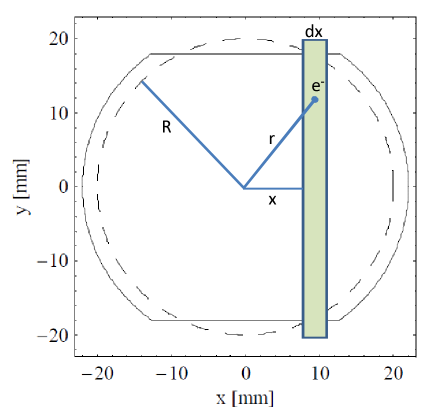
Figure 1: Cross section of the LHC screen (solid line) and the circular cross section of the pipe used in this communication (dashed line).

2 ELECTRON MOTION

In Fig. 1 the actual cross section of the LHC beam-screen together with the circular model used in this paper are shown. In the presence of a high vertical magnetic field we can consider only the transverse vertical motion of the electrons. We approximate the elicoidal trajectories as vertical straight lines since the cyclotron radius of the single particle motion is very small with respect to the transverse beam-pipe radius $R$. In this approximation, the time of flight for an electron with energy $E$ is:

$$T_{f}(E,x)=\sqrt{\frac{2m_{e}(R^{2}-x^{2})}{E}}$$ (2)

where $m_{e}$ is the electron mass.

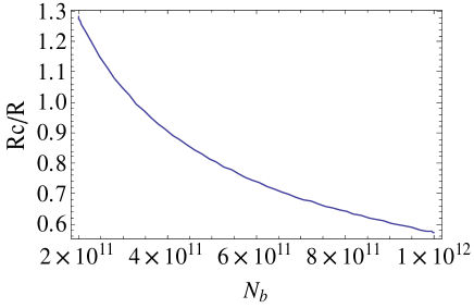
Figure 2: Critical radius as a function of bunch population.

Usually it is possible to distinguish two regimes of the electron cloud. One corresponds to electrons outside the beam core (kick regime), the other to electrons that are trapped within the beam core (autonomous regime) [5].

The former first one represents the electron motion outside the bunch during a bunch passage, and in the second one the electrons in the beam pipe perform harmonic oscillations. The critical radius $R_{c}$ separating these two regimes is defined as the radial distance for which the time for the bunch to pass is equal to a quarter of the oscillation period ($R_{c}\,=\,c\,T/4$). Hence $R_{c}$ is given as follows

$$R_{c}\,=\,\frac{\pi}{2}\sqrt{\frac{{\sigma_{r}}^{2}\,\sigma_{z}}{2\,r_{e}\,N_{b}}}$$ (3)

and it is shown in Fig. 2. The energy gain $E_{g}(x)$ is evaluated by averaging on the surface of the stripe

$$<E_{g}>\,=\,S^{-1}\int_{S}\,dS\,E(x,y)$$ (4)

where $S$ is the surface of the vertical stripe. Since $R_{c}$ is of the same order as the considered beam pipe radius, the average energy gain, for $N_{m}$ electrons uniformly distributed in a vertical stripe of the beam pipe, can be written as:

$$E_{g}(x)\,=\,\frac{\Theta(x-R_{c})}{L}\int_{0}^{L}dyE_{kick}(x,y)+\,\,\,\,\,\,\,\,\,\,\,\,\,\,\,\,\,\,\,\,\,\,\,\,\,\,\,\,\,\,\,\,$$

$$\frac{\Theta(R_{c}-x)}{L}\biggl{\{}\int_{L_{c}}^{L}dyE_{kick}(x,y)+\int_{-L_{c}}^{L}dy\frac{E_{aut}(x,y)}{2}\biggr{\}}$$ (5)

where

$$E_{kick}(x,y)\,=\,m_{e}c^{2}\frac{2{N_{b}}^{2}{r_{e}}^{2}y^{2}}{(x^{2}+y^{2})^{2}}$$ (6)

$$E_{aut}(x,y)\,=\,m_{e}c^{2}\frac{\pi^{2}\,y^{2}}{8\,{R_{c}}^{2}}$$ (7)

$L\,=\,\sqrt{R^{2}-x^{2}}$, $L_{c}\,=\,\sqrt{{R_{c}}^{2}-x^{2}}$, $N_{b}$ is the bunch population, $r_{e}$ is the classical electron radius, $\sigma_{r}$ and $\sigma_{z}$ are transverse and longitudinal beam dimensions respectively. $\Theta(x)$ is the Heaviside function. The function $E_{g}(x)$ is shown in Fig. 3 for different values of the bunch population.

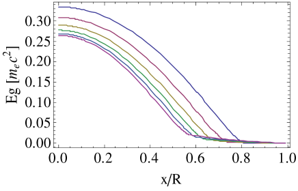
Figure 3: Energy gain as a function of the transverse distance for different values of the bunch population $N_{b}$.

3 LINEAR MAP

The electrons multiplication in the beam pipe wall is parameterized by the so-called Secondary Emission Yield (SEY or $\delta$). The total yield is the sum of the”’true secondaries”’ $\delta_{t}(E_{g})$ and ”reflected” $\delta_{r}(E_{g})$ electrons.

The $N_{m}(x)$ electrons gain an energy $E_{g}(x)$, during the passage of bunch-m, hit the chamber wall and produce $N_{m}(x)\delta_{t}$ true secondaries and $N_{m}(x)\delta_{r}$ reflected electrons. The reflected electrons travel vertically across the stripe with energy $E_{g}(x)$ and perform a number of collisions, $n(x)$, with the chamber wall, between two consecutive bunches, that is

$$n(x)\,=\,\frac{t_{sb}-T_{f}(E_{g},x)}{T_{f}(E_{g},x)}$$ (8)

where $t_{sb}$ is the bunch spacing. Hence, the total number of reflected, high energy electrons at the passage of bunch-$(m+1)$ is

$$N_{r}(x)=N_{m}(x){\delta_{r}(E_{g})}^{n(x)}$$ (9)

The true secondaries electrons produced after the first wall collision give rise to a low energy jet ($E_{sec}\approx 5eV$). For this jet there is no distinction between the true secondaries and reflected, since all are produced with the same energy. After the $i^{th}$ wall collision the number of electrons is

$$N_{t}(x)=N_{m}(x)\delta_{t}(E_{g}){\delta_{r}(E_{g})}^{i-1}\delta_{sec}^{k_{i}(x)}$$ (10)

where $\delta_{sec}=\delta_{r}(E_{sec})+\delta_{t}(E_{sec})$ and

$$k_{i}(x)=\frac{t_{sb}-iT_{f}(E_{sec},x)}{T_{f}(E_{sec},x)}$$ (11)

is the number of collisions after the $i^{th}$ collision. The low energy electrons at the passage of bunch-$(m+1)$ is

$$N_{s}(x)=N_{m}(x)\delta_{t}(E_{g})\sum_{i=1}^{n(x)}{\delta_{r}(E_{g})}^{i+1}\delta_{sec}^{k_{i}(x)}$$ (12)

Finally the total number of surviving electrons at bunch passage $(m+1)$ is obtained taking into account both the high and low energy contributions

$$N_{m+1}(x)=N_{m}(x)\left(\delta_{r}^{n(x)}+\delta_{t}\sum_{i=1}^{n(x)}\delta_{r}^{i+1}\delta_{sec}^{k_{i}(x)}\right)$$ (13)

and the linear term can be written in the form

$$a(x)\,=\,\frac{N_{m+1}(x)}{N_{m}(x)}=\delta_{r}^{n(x)}+\delta_{t}\delta_{sec}^{\eta}\frac{\delta_{sec}^{n(x)\eta}-\delta_{r}^{n(x)}}{\delta_{sec}^{\eta}-\delta_{r}^{n(x)}}$$ (14)

where $\eta=\sqrt{E_{sec}/E_{g}}$. In Fig. 4 and 5, respectively, the linear map coefficient is displayed for different values of $N_{b}$ and $\delta_{max}$.

Table 1: Parameters for LHC

parameter	unit	value
beam particle energy	GeV	7000
bunch spacing	m	7.48
bunch length	m	0.075
number of bunches $N_{b}$	–	72
number of particles per bunch $N$	$10^{11}$	1.1 to 10
bending field $B$	T	8.4
length of bending magnet	m	1
vacuum screen half height	m	0.018
vacuum screen half width	m	0.022
circumference	m	27000
primary photo-emission yield	-	$7.98\cdot 10^{-4}$
maximum $SEY$ $\delta_{max}$	-	1.3 to 2.5
energy for max. $SEY$ $E_{max}$	eV	237.125
energy width for secondary $e^{-}$	eV	1.8

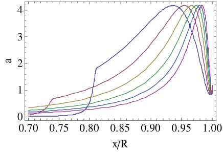
Figure 4: Linear map coefficient $a(x)$ for different values of $N_{b}$.

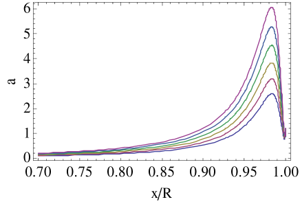
Figure 5: Linear map coefficient $a(x)$ for different values of $\delta_{max}$.

4 CONCLUSIONS

The linear map coefficient is analytically derived for the evolution of an electron cloud density inside a dipole. The analysis is useful to determine safe regions in parameter space in order to reduce the electron cloud effects.

References

- [1] U.Iriso and S.Peggs, ”Maps for Electron Clouds”, Phys.Rev. ST-AB8, 024403, 2005.
- [2] U. Iriso and S. Pegg, Proc. of EPAC06, pp. 357-359.
- [3] T. Demma and S. Petracca, Proc. of EPAC08, pp. 1601-1603.
- [4] T.Demma et al., ”Maps for Electron Clouds: Application To LHC”, Phys.Rev.ST-AB10, 114401 (2007).
- [5] J. Scott Berg, ”Energy gain in an electron cloud during the passage of a bunch”, LHC Project Note 97, CERN, Geneva (CH), 1997.
-
[6]
http://wwwslap.cern.ch/electron-cloud/Programs/Ecloud/
ecloud.html.