Dijet searches for new physics in ATLAS

Abstract

The latest results are presented of the search for new physics in inclusive dijet events recorded with the ATLAS detector. The search for resonances in the dijet mass spectrum is updated with 0.81 fb^-1 of 2011 data. The latest analysis of dijet angular distributions, with 36 pb^-1 of 2010 data, is also presented. In-depth information is provided about the model-independent search for resonances. Limits are provided for excited quarks, axigluons, scalar color octets, and to Gaussian signals that allow to set approximate limits in a model-independent way.

I Introduction

A search for new physics in events with at least two hadronic jets is motivated by numerous proposed extensions of the Standard Model (SM), ranging from quark structure to extra spatial dimensions. Experimentally, the large number of dijet events allows for a data-driven background estimation from very early.

ATLAS currently pursues two complementary searches in dijet events:

1. The search for resonances in the mass ($m_{jj}$) spectrum of the two highest-$p_{T}$ (a.k.a. “leading”) jets, PRL ; NJP

2. The search for an enhancement of leading jets produced at similar rapidities, i.e. at small $|\Delta y|$. angularPLB ; NJP

For brevity, the former analysis is called “Resonance Search”, and the latter “Angular Search”. Both are sensitive to very similar new physics that would appear in both $m_{jj}$ and $\Delta y$.

Section II offers an overview of the Angular Search and its latest results with 36 pb^-1 of 2010 data. Section III contains the latest update of the Resonance Search, with 0.81 fb^-1 of 2011 data. In Section III.1, the opportunity is taken to offer in-depth information about the method used to search for anomalies in a model-independent way, explaining hypertests and the BumpHunter BH . Section III.2 summarizes the limits set to specific models, and Sec. III.3 the model-independent limits.

II Summary of 2010 results

This Section summarizes the results of NJP , where both dijet searches were presented with 36 pb^-1 of 2010 data. Since this has been the latest update of the Angular Search, more emphasis will be given to it here, deferring the Resonance Search for later.

The event selection, which is detailed in NJP , ensures good data quality, well-measured jets, and constant trigger efficiency. The basic observable of the Angular Search is

$$\chi\equiv e^{|\Delta y|},$$ (1)

where $\Delta y$ is the rapidity difference between the leading and the subleading jet, i.e. the jet with the highest and second highest $p_{T}$ in each event. Fig. 1(a) shows the distribution of data in $\chi$, in 5 broad intervals (a.k.a. “bins”) of $m_{jj}$. The data are statistically compatible with the expectation, which is computed using Pythia Monte Carlo (MC) to model QCD, and NLOJET++ for next-to-leading-order (NLO) corrections. A derived observable is $F_{\chi}$, which is the fraction of events at $\chi<e^{1.2}$. The choice of $e^{1.2}$ is based on optimization of the sensitivity to quark contact interactions. New physics would appear as an in crease in $F_{\chi}$. When $F_{\chi}$ is computed in bins of $m_{jj}$, the result is an spectrum which can indicate new physics by an increase of $F_{\chi}(m_{jj})$ in $m_{jj}$ bins that contain significant amounts of signal. Fig. 1(b) shows the observed and expected $F_{\chi}(m_{jj})$ spectra.

No significant discrepancy is observed. The $p$-values of goodness-of-fit tests, which use as test statistic the negative logarithm of the likelihood ($L$) of the data in all bins assuming the background ($-\log L(\text{data}|\text{background})$), are of order 30% or more. This level of agreement is observed in all $m_{jj}$ bins where $\chi$ was examined, and in the $F_{\chi}(m_{jj})$ spectrum (Fig. 1).

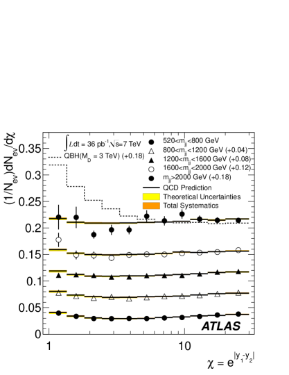
(a) The observed (filled points) and expected (histograms) $\chi$ distribution.

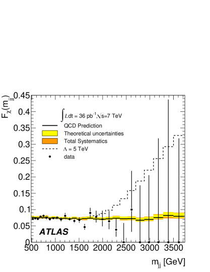
(b) The observed (filled points) and expected (histograms) $F_{\chi}(m_{jj})$ distribution.

Figure 1: Distributions of $\chi$ (left) and $F_{\chi}(m_{jj})$ (right). The dashed histogram is an example of quark compositeness signal MC.

Since agreement was found with the SM, limits were set to various new physics models. Three angular observables were used: The full $F_{\chi}(m_{jj})$ spectrum, the $F_{\chi}$ of events with $m_{jj}>2$ TeV, and the differential distribution of events in $\chi$, i.e. $\frac{dN}{d\chi}$, in events with $m_{jj}>2$ TeV. Table 1 summarizes all results, including those of the Resonance Search, which have now been superseeded by 2011 data, as will be shown. All Frequentist limits in NJP apply the classical ($CL_{s+b}$) Neyman construction Neyman with test statistic being the logarithm of the ratio of likelihoods of the hypothesis with and without signal. Systematic uncertainties are mainly from the jet energy scale, the renormalization and factorization scales ($\mu_{R}$,$\mu_{F}$), and parton density functions (PDF). These uncertainties are propagated to the limits by random sampling of the nuisance parameters, making thus the Neyman band wider, which is known to not be fully conistent with the Frequentist framework, but is a practice accepted as common. Regarding in particular the limit on contact interaction scale $\Lambda$ using $F_{\chi}(m_{jj})$, the observed Frequentist limit of 9.5 TeV is much above the expected limit. However this is not the case for the Bayesian limit using the same $F_{\chi}(m_{jj})$, or for the Frequentist limits using the other two angular observables (see last 4 rows of Table 1).

Table 1: Lower limits, at 95% confidence level (or credibility level, for Bayesian limits) (C.L.), set by the Resonance and Angular Search in 36 pb^-1 of 2010 data NJP . Results of the Angular Search are distinguished by the observable listed in the first column. The second column lists which limits are Frequentist and which Bayesian (with a constant prior in signal cross-section for the Resonance Search, and in $\frac{1}{\Lambda^{2}}$ for the Angular Search).

Analysis / observable	Method	95% C.L. Limits (TeV)
		Expected	Observed
Excited Quark $\bf{q^{\ast}}$
Resonance in $m_{jj}$	Bayesian	2.07	2.15
$F_{\chi}(m_{jj})$	Frequentist	2.12	2.64
Randall-Meade Quantum Black Hole for $\bf n=6$
Resonance in $m_{jj}$	Bayesian	3.64	3.67
$F_{\chi}(m_{jj})$	Frequentist	3.49	3.78
$F_{\chi}$  for $m_{jj}>2$ TeV	Frequentist	3.37	3.69
$\frac{dN}{d\chi}$ for $m_{jj}>2$ TeV	Frequentist	3.46	3.49
Axigluon
Resonance in $m_{jj}$	Bayesian	2.01	2.10
Contact Interaction $\bf\Lambda$
$F_{\chi}(m_{jj})$	Frequentist	5.7	9.5
$F_{\chi}(m_{jj})$	Bayesian	5.7	6.7
$F_{\chi}$ for $m_{jj}>2$ TeV	Frequentist	5.2	6.8
$\frac{dN}{d\chi}$ for $m_{jj}>2$ TeV	Frequentist	5.4	6.7

III Dijet Resonance Search with 0.81 fb^-1 of 2011 data

This section is a summary of resonancePLB , that highlights some of the technical details of the analysis.

The main observable is $m_{jj}$, the mass of the system of the two leading jets in $p_{T}$. Events are selected to ensure good beam and detector conditions, well-reconstructed leading jets, no potential of accidental swapping of the order of jets in $p_{T}$, and constant trigger efficiency in $m_{jj}$. To suppress the QCD background at high mass, the $|\Delta y|$ is required to be less than 1.2, in accordance with the Angular Analysis (Section II).

The $m_{jj}$ spectrum is compared to the expected, searching for a local enhancement of the cross-section around some value of $m_{jj}$, which is what “resonance” means in this context. The comparison is made by a hypertest known as BumpHunter BH . Bayesian lower limits are set, at 95% credibility level (C.L.), on the mass of excited quarks exq , axigluons axg , and scalar color octets TaoHan . Finally, model-independent limits are given, which can be used to approximate the limit to virtually any resonant signal decaying into two jets.

The expected spectrum is obtained by fitting to the data the function

$$f(x)=p_{0}\frac{(1-x)^{p_{1}}}{x^{p_{2}+p_{3}\ln x}},\hskip 4.26773pt\text{where\ \ }x\equiv\frac{m_{jj}}{\sqrt{s}}.$$ (2)

This parametrization has been shown to fit well the QCD prediction given by Pythia, Herwig, Alpgen, and NLOJET++ CDFanalysis . Figure 2 shows an example of fitting the Pythia QCD prediction, after full ATLAS detector simulation, without NLO corrections.

The fit is performed in such a way that, if the data contains non-negligible signal in any $m_{jj}$ interval, that will be omitted from the fit, thus obtaining the background from the sidebands. The algorithm that determines if that is necessary searches for any $m_{jj}$ window that may be responsible for a globally poor fit ($\chi^{2}$ test $p\mbox{-value}$ $<$ 1%). No such interval was found in the data, so, the whole spectrum was fitted, giving a $\chi^{2}$ $p\mbox{-value}$ much greater than the 1% threshold.

Figure 2 shows the data, along with the fitted background, and three examples of $q^{\ast}$ signal added to it. The overall consistency of the data with the fit is quantified by the $p\mbox{-value}$ of the negative logarithm of the likelihood of the data when the background is expected ($-\log L(\text{data}|\text{background})$). This is a generalization of the $\chi^{2}$ test that accounts correctly the Poisson probability in bins with low background. That $p\mbox{-value}$ is about 13%, indicating consistency.

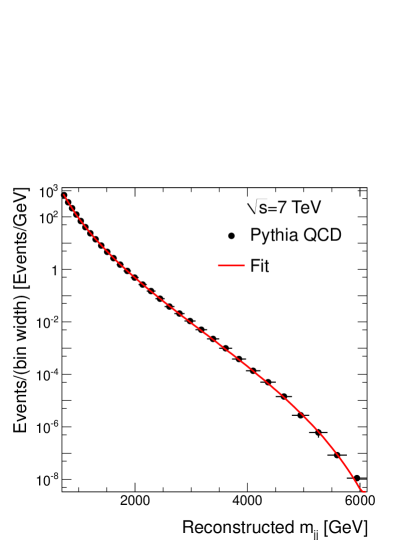
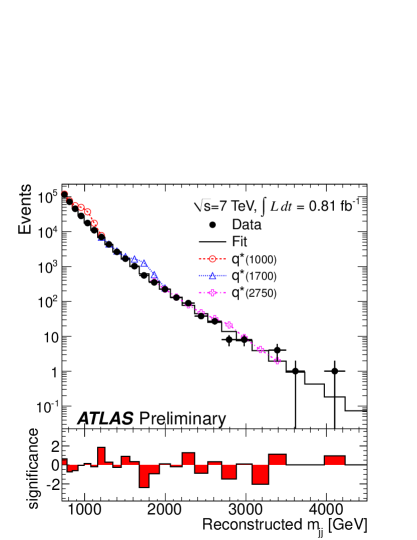
Figure 2: Left: The function of eq. 2 used to fit Pythia QCD, after ATLAS detector simulation. Right: The data (black markers), the fitted background (solid histogram), and three examples of $q^{\ast}$ signal (hollow markers). The red bars indicate the significance of each excess (positive bars) or deficit (negative bars) of data, expressed in standard deviations PDG . In bins with small expected number of events, where the observed number of events is similar to the expected, the Poisson probability of a fluctuation at least as high (low) as the observed excess (deficit) can be greater than 50%, resulting in a negative significance when expressed in standard deviations. Drawing negative values would obscure the current intuitive convention that data excesses appear as positive bars and data deficits as negative bars, and the amplitude of each bar is proportional to the significance of each deviation. Such bins present no statistical interest, so, for simplicity, bars are not drawn for them.

III.1 The model-independent search for resonances

The BumpHunter algorithm BH is used to look for resonances in the $m_{jj}$ spectrum in a model-independent way, which offers high sensitivity, and takes correctly into account the trials factor (a.k.a. “look elsewhere” effect), namely the effect of examining various positions of the $m_{jj}$ spectrum before eventually finding something. The general way to account for the trials factor is to construct a hypertest, and the BumpHunter is just one such hypertest.

In BH one can find a detailed account of the trials factor, the definition of hypertests, and details about the BumpHunter and other similar hypertests, such as the TailHunter. A summary is given here.

A hypertest is a hypothesis test, much like the well-known $\chi^{2}$ or the Kolmogorov-Smirnov (KS) test. It has a test statistic, and a corresponding $p\mbox{-value}$, which is, as usual, the frequency with which a more signal-like test statistic than the one observed in data would occur under the background-only hypothesis. The difference is that, in a hypertest, the test statistic itself is a $p\mbox{-value}$ , therefore the $p\mbox{-value}$ of a hypertest is a $p\mbox{-value}$ of a $p\mbox{-value}$. Each hypertest contains in its definition an ensemble of hypothesis tests. These are the hypertest’s “members”, and their multitude is responsible for the trials factor. The hypertest combines the results of its members. The hypertest’s test statistic is, by convention, the negative logarithm of the smallest $p\mbox{-value}$ of all tests in the ensemble. The $p\mbox{-value}$ of the hypertest is the frequency by which, in the background-only hypothesis, there would be any test in the ensemble with a $p\mbox{-value}$ at least as small as the smallest $p\mbox{-value}$ found in the ensemble of tests when they were performed on the actual data.

The BumpHunter, as implemented in this analysis, is a hypertest whose ensemble of combined tests is defined after forming all possible $m_{jj}$ intervals in the binned $m_{jj}$ spectrum, and performing in each interval a simple event-counting hypothesis test. The bin sizes increase at higher $m_{jj}$, following detector resolution, such that any new physics signal would populate at least two consecutive bins. For this reason, we do not consider $m_{jj}$ intervals narrower than two bins. Since we are only interested in excesses of data, the test statistic of the hypothesis test performed in each $m_{jj}$ interval takes its minimum value, which is 0 by convention, if the data in the interval ($D$) are fewer than expected ($B$). If $D>B$, then the test statistic increases monotonically with $D-B$, for example as $(D-B)^{2}$, or $(D-B)^{100}$, or $-\log(\frac{B^{D}}{D!}e^{-B})$; it doesn’t matter exactly how the test statistic increases, because all the hypertest needs is the $p\mbox{-value}$ of this test statistic, which in any case is the Poisson probability of observing at least $D$ events when $B$ are expected: $\sum_{n=D}^{\infty}\frac{B^{D}}{D!}e^{-B}$.

An equivalent, more procedural (and maybe more intuitive) way to describe the BumpHunter hypertest is the following algorithm:

1. Scan the $m_{jj}$ spectrum, counting events in all intervals of at least 2 bins, and in each interval compute the Poisson $p\mbox{-value}$ of seeing at least as many data as observed, given the expected number of events.

2. Keep the smallest Poisson $p\mbox{-value}$ found in the actual data. This number is the observed test statistic of the BumpHunter.

3. Generate many spectra of background-only pseudo-data, and scan them too, noting the smallest Poisson $p\mbox{-value}$ in each one. Note that, since the data were compared to the background fitted to them, the fit must be repeated to each individual pseudo-spectrum before scanning. This wouldn’t be necessary if the background was not obtained by a fit.

4. Measure how frequently a pseudo-spectrum returns a minimum Poisson $p\mbox{-value}$ that is smaller than the observed test statistic (step 2). This frequency is the $p\mbox{-value}$ of the BumpHunter hypertest.

If the BumpHunter’s $p\mbox{-value}$ is very small it is a fail-safe statement to say that there is a local excess in the data, which is incompatible with the background, because the probability of such an excess being pure coincidence is equally small. It also helps that we know which member test (i.e. which $m_{jj}$ interval) returned the smallest $p\mbox{-value}$, because that is where the signal is, so we are pointed at it.

By its very construction, a hypertest accounts for the trials factor, since it considers every member test in every pseudo-experiment.

It is very important that the hypertest’s test statistic is the largest $-\log(p\mbox{-value})$ in the ensemble, e.g. the largest

$$-\log\left(\sum_{n=D}^{\infty}\frac{B^{n}}{n!}e^{-B}\right),$$ (3)

and not the largest test statistic in the ensemble, e.g. the largest

$$-\log\left(\frac{B^{D}}{D!}e^{-B}\right),\mbox{ or }(D-B)^{100}.$$ (4)

It would have been wrong to use directly the test statistic of the most discrepant member test, because test statistics of different member tests follow different distributions under the background-only hypothesis, and are not comparable. For example, in the case of the BumpHunter, this mistake could have led to a hypertest with strong bias towards low $m_{jj}$ regions with high background ($B$), because, e.g., $(1010-1000)^{100}$ is greater than $(15-10)^{100}$, even though it’s obvious that observing 1010 events instead of 1000 is less significant than observing 15 instead of 10. The right way to combine dissimilar hypothesis tests is by comparing their $p$-values, not their test statistics. Hypertests, by construction, avoid this pitfall.

Figure 3 demonstrates the sensitivity of the BumpHunter to a test signal injected at 2 TeV, with Gaussian shape of standard deviation 100 GeV (Fig. 3(a)). Figure 3(b) compares the power of a variety of hypothesis tests, defined as the probability a test has to observe a $p\mbox{-value}$ less than 5% (equivalent to a 1.6$\sigma$ effect), as a function of the expected number of injected signal events. The faster the power increases, the higher the sensitivity of a test to this signal.

In Fig. 3(b), two of the compared tests, the BumpHunter and the TailHunter BH , are hypertests with no knowledge of the injected signal. The rest are not hypertests. Three of them examine the whole spectrum: the KS test, the $\chi^{2}$ test, and its generalization that uses the test statistic $-\log(\prod_{\text{bins}}\frac{B^{D}}{D!}e^{-B})$. Finally, two hypothesis tests are constructed exploiting knowledge of the signal, which in reality is not possible, unless one knows in advance what is about to be discovered. One of these two tests is aware only of the signal location, so, it performs a counting test just in the bins where 68% of the signal is expected. The other knows the exact shape and position of the signal, but not how much it is, so it uses as test statistic the $\log\left(\frac{L(\text{data}|\hat{s})}{L(\text{data}|\text{no signal})}\right)$, where $\hat{s}$ is the best fitting amount of the known signal.

The comparison shows that, among the tests with no prior knowledge of the signal, the BumpHunter is by far the most sensitive, followed by the TailHunter. This is true despite the trials factor, which does not apply to other tests. The KS test is the least sensitive to this signal. The most sensitive test of all is the one which knows the exact shape and position of the signal. The next most sensitive is the one that knows its position.

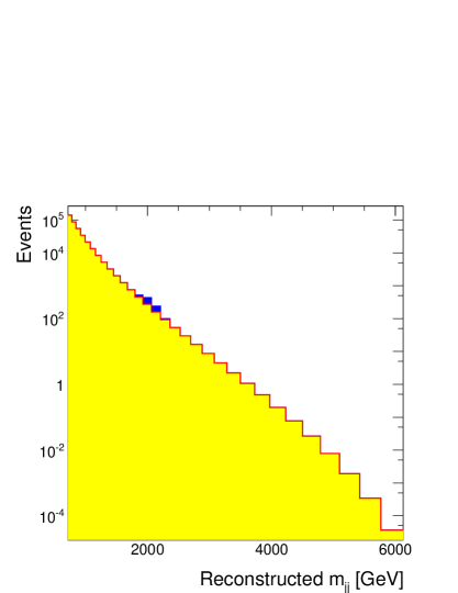
(a) Toy background and signal

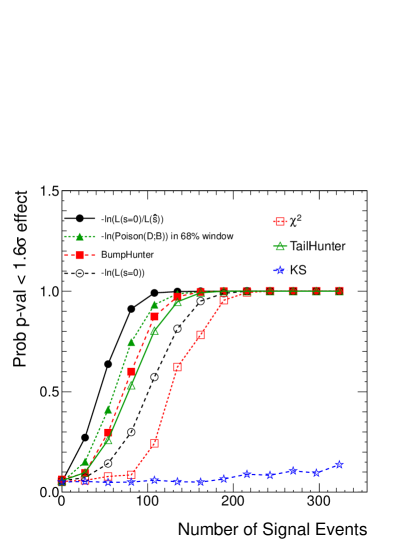
(b) Power of tests

Figure 3: Left: The toy signal (blue, Gaussian at 2 TeV with $\sigma$=100 GeV) injected on top of a background similar to QCD. Right: The power (see text) of the following tests, as a function of injected signal events: The BumpHunter (filled squares), the TailHunter BH (empty triangles), the KS test (stars), the $\chi^{2}$ test (empty squares), its generalization that uses the negative logarithm of the likelihood of the data under the background-only hypothesis (empty circles), and two tests that know something about the injected signal: a test that performs event-counting in the windw which contains 68% of the signal (filled triangles), and a test that knows not only the position, but also the exact shape of the signal, and computes a likelhood ratio test statistic (filled circles).

III.1.1 Results of the search for resonances

Figure 4(a) shows the most interesting interval identified by the BumpHunter in the actual data. Figure 4(b), known as “BumpHunter tomography”, shows $\sum_{n=D}^{\infty}\frac{B^{n}}{n!}e^{-B}$ in each $m_{jj}$ interval that contains an excess of data ($D>B$), which allows us to see that there is no interval that gets anywhere close to being significant, even without accounting for the trials factor. Figure 4(c) shows the distribution of the BumpHunter test statistic under the background-only hypothesis, and the blue arrow indicates the observed test statistic value. From that it is clear that the observed spectrum does not contain any significant bump anywhere. The BumpHunter’s $p\mbox{-value}$ is 62%.

No significant excess has been found in $m_{jj}$ in 0.81 fb^-1 of data.

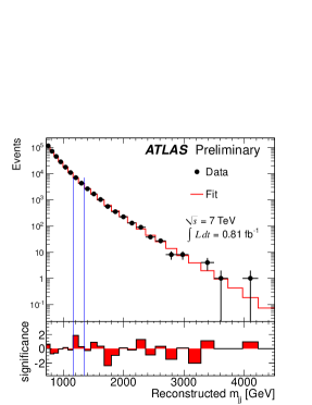
(a) Most discrepant interval

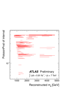
(b) BumpHunter tomography plot

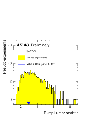
(c) Distribution of test statistic

Figure 4: Results of the search for resonances. Left: The most significant excess found in the data, indicated by the blue vertical lines. Middle: The Poisson $p\mbox{-value}$ ($\sum_{n=D}^{\infty}\frac{B^{n}}{n!}e^{-B}$ in each interval with an excess ($D>B$). Each $m_{jj}$ interval is indicated by its position in the horizontal axis, and its $p\mbox{-value}$ by the position on the vertical axis. Even the most significant interval, without any trials factor to be considered, has a $p\mbox{-value}$ of about 0.09, which is very insignificant. Right: The distribution of the BumpHunter test statistic under the background-only hypothesis, compared to the observed test statistic (blue arrow). The BumpHunter $p\mbox{-value}$ is 62%.

III.2 Limits to specific models

Upper limits are set to the accepted cross-section ($\sigma\times\mathcal{A}$) of excited quarks ($q^{\ast}$), axigluons ($A$), and scalar color octets ($s8$). Details about how these models were simulated can be found in resonancePLB . The limits are Bayesian, at 95% credibility level, with a constant prior in $\sigma\times\mathcal{A}$. The observed and expected limits are compared to the corresponding theoretical predictions in Fig. 5. Lower mass limits are summarized in Table 2.

The main systematic uncertainties, which have been convolved to the limits, are the jet energy scale (JES) uncertainty (2 to 4%, depending on $p_{T}$ and $\eta$), the background fit uncertainty (ranging from less than 1% at the beginning of the spectrum, and reaching about 20% at 4 TeV), and the luminosity uncertainty of 4.5%. The jet energy resolution (JER) uncertainty has a negligible effect on the limits and is ignored.

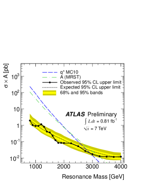
(a) Limits to $q^{\ast}$ and $A$

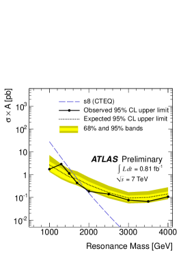
(b) Limits to $q^{\ast}$ and $A$

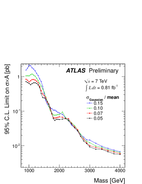
(c) Limits to Gaussians

Figure 5: Limits to excited quarks and axigluons (left), to scalar color octets (middle), and to Gaussian-distributed signals (right) of mean values between 900 GeV and 4 TeV and standard deviations ($\sigma_{\rm Gaussian}$) from 5% to 15% of the mean value.

Table 2: The 95% CL mass lower limits for the models examined in this study.

Model	95% CL Limits (TeV)
	Expected	Observed
Excited Quark	2.77	2.91
Axigluon	3.02	3.21
Colour Octet Scalar	1.71	1.91

III.3 Model-independent limits

In addition to specific theories, limits are also set to a collection of hypothetical signals that are assumed to be Gaussian-distributed in $m_{jj}$, with means ranging from 0.9 to 4.0 TeV, and standard deviations from 5% to 15% of the mean. These limits include the same luminosity and background fit systematic uncertainties. Since the Gaussian $m_{jj}$ distributions do not result from actual jets, to convolve the JES uncertainty the mean of the Gaussian is given a 4% uncertainty, which is conservatively larger than the shift observed in $q^{\ast}$ templates when jet $p_{T}$ was shifted by the JES uncertainty.

The results are shown in Fig. 5(c). These limits can be used to set approximate limits on any new physics model that predicts some peaking signal in $m_{jj}$, because almost every signal excess can be approximated by a Gaussian at some level. A procedure is given in resonancePLB , to make the approximation. The non-Gaussian tails of the signal need to be removed, to make the Gaussian shape a better approximation to the remaining signal. Removing the tails results in lower signal acceptance. Removing the tails does not affect the much the mass limits, because the tails are in background-dominated regions; the theoretical cross-section of the new particle is reduced by the acceptance of keeping just the core of its $m_{jj}$ distribution, but the $\sigma\times\mathcal{A}$ upper limit is reduced by roughly the same fraction, so, the theory and the limits continue to intersect at the same mass as if the tails had not been removed.

IV Conclusion

The latest results were shown, from the new physics searches in the dijet angular and mass distribution. The latter was updated with 0.81 fb^-1 of 2011 data. No sign of new physics was found. Limits to $q^{\ast}$ improved by about 1 TeV since 2010, and are the most stringent ones currently. Limits to Gaussian signal distributions have been updated, as a tool to compute approximate limits to more theoretical models.

- (1) ATLAS Collaboration, Search for New Particles in Two-Jet Final States in 7 TeV Proton-Proton Collisions with the ATLAS Detector at the LHC, Phys. Rev. Lett. 105, 161801 (2010).
- (2) G. Choudalakis, Early Searches with Jets with the ATLAS Detector at the LHC, PoS(ICHEP 2010)387.
- (3) ATLAS Collaboration, Search for Quark Contact Interactions in Dijet Angular Distributions in pp Collisions at = 7 TeV Measured with the ATLAS Detector, Phys.Lett.B694:327-345,2011.
- (4) G. Choudalakis, On hypothesis testing, trials factor, hypertests and the BumpHunter, arXiv:1101.0390 [physics.data-an].
- (5) ATLAS Collaboration, Search for New Physics in Dijet Mass and Angular Distributions in Collisions at TeV Measured with the ATLAS Detector, New J. Phys. 13 (2011) 053044.
- (6) Neyman, J., Outline of a Theory of Statistical Estimation Based on the Classical Theory of Probability, Philosophical Transactions of the Royal Society of London. Series A, Mathematical and Physical Sciences, vol. 236 (767), pages 333-380, 1937.
- (7) U. Baur, I. Hinchliffe, and D. Zeppenfeld, Int. J. Mod. Phys. A2, 1285 (1987).
- (8) P. Frampton and S. Glashow, Phys. Lett. B 190, 157 (1987).
- (9) T. Han, I. Lewis, and Z. Liu, JHEP 12, 085 (2010), arXiv:1010.4309 [hep-ph].
- (10) CDF Collaboration, Search for new particles decaying into dijets in proton-antiproton collisions at = 1.96 TeV, Phys.Rev.D79:112002,2009.
- (11) ATLAS Collaboration, Search for New Physics in Dijet Mass Distributions in 0.81 fb-1 of Collisions at =7 TeV, ATLAS-CONF-2011-095.
- (12) K. Nakamura et al. (Particle Data Group), J. Phys. G 37, 075021 (2010), equation 33.33.