HST Observations of the Stellar Distribution Near Sgr A^∗

Abstract

Sgr A^∗ is embedded within the nuclear cluster, which consists of a mixture of evolved and young populations of stars dominating the light over a wide range of angular scales. Here we present HST/NICMOS data to study the surface brightness distribution of stellar light within the inner 10^′′ of Sgr A^∗ at 1.45$\mu$m, 1.7$\mu$m and 1.9$\mu$m. We use these data to independently examine the surface brightness distribution that had been measured previously with NICMOS and to determine whether there is a drop in the surface density of stars very near Sgr A^∗. Our analysis confirms that a previously reported drop in the surface brightness within 0.8^′′ of Sgr A^∗ is an artifact of bright and massive stars near that radius. We also show that the surface brightness profile within 5^′′ or $\sim$0.2 pc of Sgr A^∗ can be fitted with broken power laws. The power laws are consistent with previous measurements, in that the profile becomes shallower at small radii. For radii $>$ 0.7^′′, the slope is $\beta=-0.34\pm 0.04$ where $\Sigma$ is $\propto r^{\beta}$ and becomes flatter at smaller radii with $\beta=-0.13\pm 0.04$. Modeling of the surface brightness profile gives a stellar density that increases roughly as r^-1 within the inner 1^′′ of Sgr A^∗. This slope confirms earlier measurements in that it is not consistent with that expected from an old, dynamically-relaxed stellar cluster with a central supermassive black hole. Assuming that the diffuse emission is not contaminated by a faint population of young stars down to the 17.1 magnitude limit of our imaging data at 1.70$\mu$, the shallow cusp profile is not consistent with a decline in stellar density in the inner arcsecond. In addition, converting our measured diffuse light profile to a stellar mass profile, with the assumption that the light is dominated by K0 dwarfs, the enclosed stellar mass within radius $r\lower 1.72218pt\hbox{$\;\buildrel<\over{\scriptstyle\sim}\;$}0.1$ pc of Sgr A* is $\approx 3.2\times 10^{4}$ M${}_{\odot}(r/0.1\,\mathrm{pc})^{2.1}$.

1 Introduction

There is compelling evidence that the compact radio source Sgr A^∗ is located at the very dynamical center of our galaxy (Reid & Brunthaler 2004) and coincides with a $4\times 10^{6}$$M_{\odot}$ black hole (Ghez et al. 2009; Gillessen et al. 2009). The nuclear cluster surrounding Sgr A^∗ consists of a mixture of an evolved stellar population, probably having an isotropic stellar light distribution (Trippe et al. 2008; Schödel et al. 2009), and a young population of stars at smaller radii from Sgr A^∗. Sgr A^∗ is known to be less energetic and massive than black holes in luminous active galactic nuclei (AGN), which can outshine the brightness of their nuclear clusters. Given the low luminosity of Sgr A^∗ and its proximity, high spatial resolution observations of the nuclear cluster provide an unparalleled opportunity to observe in detail the influence of the central black hole on the spatial distribution of stars and to test theories of cusp formation.

Peebles (1972) showed that the signature of a central black hole in a dense stellar cluster is a cusp with a power law form of $\rho\propto r^{\gamma}$. Follow-up studies indicate that the power law slopes can range from $\gamma$=–3/2 to –7/4 depending on whether the mass of stars dominating the stellar density profile is neutron stars, white dwarfs, or stellar black holes, respectively (Bahcall and Wolf 1976, 1977; see reviews by Merritt 2006, Alexander 2005; Genzel et al. 2010). Numerical simulations suggest that if the stellar cluster is dynamically relaxed, it should have a cusp with a power law slope in density of $-$2 for massive stars and and $-$1.5 for low mass stars (Hopman & Alexander 2006; Preto & Amaro-Seoane 2010).

Due to its proximity, the Galactic center is an ideal place to examine the influence of Sgr A^∗ on the spatial distribution of evolved stars. Late-type K and M giant stars could be used as good tracers of cusp dynamics, assuming they are older than the relaxation time scale (Alexander et al. 2007; Schödel et al. 2007; Merritt 2010). Numerous measurements have been carried out over the years to study the infrared distribution of stars in the vicinity of Sgr A^∗ and investigate the power law distribution of evolved stars in the hope of finding evidence for a stellar cusp. The study by Becklin & Neugebauer (1968) revealed that on parsec size scales the surface brightness ($\Sigma$) profile is a power law. Numerous follow-up studies confirmed that the slope beyond the projected distance r=0.5pc follows a power law slope of $\beta$=–0.8, where $\Sigma$ $\propto r^{\beta}$ ($\gamma$=$\beta$+1) (e.g., Catchpole, Whitelock, & Glass 1990; McGinn et al. 1989; Rieke and Rieke 1994; Haller et al. 1996). The signature of a stellar cusp, however, should be seen within the inner 0.5pc, it has proved more challenging to measure the slope because of source crowding, the presence of bright stars and possible differential extinction. Early studies indicated that stellar number density measurements show a flat stellar cluster within a projected radius of 0.2–0.3pc (McGinn et al. 1968; Eckart et a. 1993; Haller et al. 1996; Launhardt et al. 2002). Follow-up studies used Adaptive Optics (AO) to improve the sensitivity and spatial resolutions and determined that the volume density of stars within $\sim$0.25–0.35 pc increases toward Sgr A^∗ with $\gamma\sim$-1.3 to -1.4 (Genzel et al. 2003). Using better quality data and improved methods of analysis, Schödel et al. (2007) estimated the power law slope $\gamma=-1.2\pm 0.05$ at a projected radius of 6^′′. This slope is not consistent with that expected from an old, dynamically-relaxed stellar cluster with a central supermassive black hole.

Unlike the technique of measuring stellar density counts of stars, Scoville et al. (2003) used HST/NICMOS images to measure the diffuse stellar emission near Sgr A^∗, determining the radial distribution of observed and extinction-corrected 1.9$\mu$m emission. The spatial variation of extinction was determined by using Pa$\alpha$, radio continuum and radio recombination line measurements. The greatest difference between the observed and extinction-corrected distribution occurs at projected radii $>$10^′′ (corresponding to deprojected radii $\sim$30^′′), where the larger extinction corrections associated with the circumnuclear molecular ring raises the extinction-corrected flux by a greater amount. They showed that the observed and extinction-corrected 1.9$\mu$m surface brightness distribution increases strongly inwards to a projected radius of 1^′′ and then exhibits a drop within 0.8^′′ of Sgr A^∗. The drop in the surface brightness distribution is an important parameter to determine accurately. This feature could have several different origins: it might be the core radius of the nuclear stellar distribution, it might be due to the depletion of late-type stars with high mass-to-light ratios (e.g., Bailey & Davies 1999), or due to depletion of giant stars through collisions with main-sequence stars (Genzel et al. 1996; Sellgren et al. 1990), or even ejection of stars from the central 1^′′ by a past or present binary black hole (Hansen & Milosavljevic 2003; Yu & Tremaine 2003).

The ideas explaining the depletion of late-type stars remained viable, as described below, but the drop in the stellar surface brightness was shown to be due to artifacts of bright, massive stars that had not been subtracted properly. Schödel et al. (2007) suspected that light density in the HST images is dominated by the brightest stars and the wings of the PSF from the brightest stars. They created artificial images from the stellar number counts, to which they applied the method of Scoville et al. (2003). The comparison led Schödel et al. (2007) to conclude that the excess light density found by Scoville et al. (2003) at a projected distance of 1–5^′′, corresponding to projected radii of 0.039 and 0.4 pc at the 8 kpc distance to the Galactic center, was an artifact due to contamination of bright, young stars. These bright stars are now known to be associated with a clockwise rotating thick stellar disk, with surface density scaling as the inverse square of the true distance from Sgr A^∗ (Genzel et al. 2003; Paumard et al. 2006; Bartko et al. 2010), making the true surface brightness distribution of the evolved cluster difficult to measure. The projected inner radius of the clockwise disk is $\sim$0.3 pc or $\sim$8^′′ from Sgr A^∗, and the stellar ages are estimated to be $\sim$6 Myr, with the total mass of stars amounting to $\sim 1.5\times 10^{4}\hbox{$M_{\odot}$}$ (Paumard et al. 2006).

The nuclear cluster at the Galactic center is unique in that the cluster can be resolved down to scales of milli-pc with AO measurements. However, the distribution of bright, young massive stars, which are not dynamically relaxed, creates difficulty in testing the cusp formation near Sgr A^∗. Apart from the fact that confusion limits the detection of stars fainter than K$\sim$18–19, an additional factor that limits measurements of the radial profile of the evolved cluster is identification of the young population of stars embedded within the nuclear cluster. Earlier studies used broad-band imaging to determine the radial profile of stellar light near Sgr A^∗. Using imaging techniques, Schödel et al. (2007) determined a broken power-law distribution of stars with a break radius of $\sim$6^′′. At radii $r<6$^′′, the surface number density profile $\Sigma$(r) is fitted by a power-law index $\beta=-0.19\pm 0.05$, which is flatter than $\beta=-0.75\pm 0.1$ at $r>6$^′′. More recently, three separate studies have used narrow-band imaging (CO bandhead) or spectroscopy to separate the young and evolved stellar populations in the central 1^′′, so that the radial profile of the evolved stellar system can be distinguished and measured accurately, thus allowing theories of cusp formation to be tested. Strong CO bandhead absorption features in late type stars are used to distinguish them from early-type stars. Buchholz et al. (2009), following earlier studies by Genzel et al. (2003), used deep CO bandhead images (K $<$ 15.5) and found a shallow slope $\beta=0.17\pm 0.09$. Genzel et al. (2003) had shown that the fraction of late-type stars decreases between distances of 10 and 1^′′ from Sgr A^∗. In another study, Do et al. (2009) used the Br$\gamma$ and NaI lines of stellar sources with K${}^{\prime}<$15.5 to distinguish between early and late-type stars. They also found a shallow slope of evolved stars with $\beta=0.27\pm 0.19$. Lastly, Bartko et al. (2010) used SINFONI to make spectroscopic identification of late-type and early-type stars using both CO bandheads and Br$\gamma$ lines. This study also showed a dearth of late-type stars at small distances from Sgr A^∗. All of these results contradict earlier evidence for the signature of a cusp, and confirm a depletion in the number density of stars close to Sgr A^∗ (Genzel et al. 2003; Paumard et al. 2006; Schödel et al. 2007; Buchholz et al. 2009; Do et al. 2009; Bartko et al. 2010). These measurements indicate that the stellar light distribution of evolved stars approaching Sgr A^∗ becomes even shallower than that measured by Schödel et al. (2007), implying a deficiency of evolved stars.

A disadvantage of the NICMOS images is the relatively low spatial resolution, which can make contamination from the extended PSF wings of bright stars a problem. AO measurements have a clear advantage over HST images in that they can detect individual point sources. Another disadvantage of HST/NICMOS data is that it does not have spectroscopic capability to distinguish between late and early type stars. However, measuring the surface brightness distribution using NICMOS images has advantages because of its sensitivity to low surface brightness diffuse light, the high Strehl ratio of the imaging, and PSF stability.

The surface brightness distribution of extended and diffuse features are measured as a function of the projected distance from SgrA*. This type of measurements can especially be useful within 1^′′ (0.04pc) of Sgr A^∗, where limited number of resolved stellar sources are detected.

There are limited non-AO measurements of the surface brightness distribution of stars at the Galactic center that have been attempted. In particular, the distribution of stars is not sampled well within 1^′′ of Sgr A^∗, because there are so few stars that can be identified spectroscopically within a limiting magnitude of K$\sim$15.5. The functional form of the distribution of stars has therefore been uncertain. Here we study the surface brightness distribution at 1.45$\mu$m, 1.7$\mu$m and 1.9$\mu$m using NICMOS data originally obtained in September 2004 and April 2007 to monitor the near-IR flaring activity of Sgr A^∗. Measurements presented here use a more extensive data set compared to that of Scoville et al. (2003). In addition, a different technique has been used to remove the bright and massive stars from the surface brightness measurements, as discussed in detail in the next section.

2 Data Reduction and Analysis

For this study we have used NICMOS imaging obtained in September 2004 and April 2007, as part of Sgr A^∗ monitoring campaigns (HST GO programs 10179 and 10859, respectively). All of the exposures used NICMOS camera 1, which has a pixel scale of 0.043^′′ and a field of view of $11^{\prime\prime}\times 11^{\prime\prime}$. From the April 2007 data set we have used images obtained in the medium-band filters F145M and F170M, which have central wavelengths of 1.46$\mu$m and 1.71$\mu$m, respectively, and a FWHM of 0.2$\mu$m. From the September 2004 data set, we have used images obtained in the narrow-band F190N filter, which has a central wavelength of 1.90$\mu$m and a FWHM of 0.02$\mu$m. There are 320 exposures of 144 sec duration for each of the F145M and F170M filters, for a total exposure time of 768 minutes (12.8 hours) in each filter. For the F190N data, there are 64 exposures of 448 sec duration, for a total exposure time of 478 minutes (8 hours).

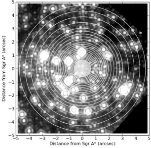
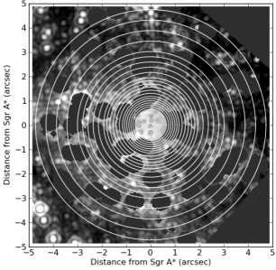
Figure 1: (a) Top Left A greyscale image of the inner 10^′′ of the Galactic center centered on the position of Sgr A^∗ at the wavelength of 1.7$\mu$m. A series of photometry apertures are overlaid on the image in order to determine the surface brightness as a function of radius. Each pixel in the image is 0.043^′′. (b) Top Right Similar to (a) except that the bright stars have been masked. (c) Bottom Left A close-up view of the inner 1^′′ of the Galactic center is shown. The brightest stars are members of the S cluster. The overlaid photometry apertures are also shown. (d) Bottom Right Similar to (c) except that the bright S stars, including S0-2, have been masked. The stars S34+S35 at the southwest corner are considered to be evolved and have not been masked.

The sets of calibrated exposures for each filter were combined into a single image using the STScI program “multidrizzle”. Multidrizzle not only combines the aligned individual exposures, but also rejects outliers (e.g. cosmic ray hits) and removes the geometric distortions of the NICMOS optics. An example of the final F170M image is shown in Figure 1a.

The radial distribution of surface brightness in the three combined images was measured by performing aperture photometry using a routine written in Python, which duplicates the methods used in standard routines like the IRAF task “phot”. The custom Python routine allowed us to explore the results from various measurement methods, as discussed below. Photometry was performed in a series of concentric circular apertures of increasing radius, centered on the position of Sgr A^∗. The surface brightness as a function of radius was then computed from the signal in the annuli formed by each adjacent pair of apertures.

Our goal is to measure the surface brightness of the relaxed stellar cluster surrounding Sgr A*, which is, unfortunately, contaminated by the light from bright, young stars. Stars fainter than K 15.5-16 within the innermost arcseconds of Sgr A* are difficult to classify, nor do we have the ability to resolve individual stars of this brightness in the HST images. Hence the best we can do to remove the contribution of the young stars is to at least remove the light from the brightest ones that we can resolve. The remaining diffuse light could have contributions from stars as young as types B to A, but we will assume for the sake of simplicity that it is dominated by the more numerous old population. There are several ways in which this could be done. First, the bright, young stars could be removed from the combined images in each filter band by PSF fitting and subtraction techniques. The NICMOS camera 1 PSF, however, is quite complex and spatially-variant. Given the extreme crowding in our images, it is virtually impossible to fit the PSF to a sufficient level of accuracy to remove the more complex features, which was verified by several different PSF subtraction attempts. Another way to remove the contribution from bright stars is to simply not include their signals when summing the data within the photometry apertures. In the study by Scoville et al. (2003), for example, which also used NICMOS images to measure the surface brightness distribution around Sgr A^∗, photometry was computed from the median pixel value after rejecting the brightest 20% of the pixels within each annulus. While this helps to remove some of the effect of bright stars, it has the drawback of using a varying rejection threshold in each annulus. Annuli containing very bright stars will have a much higher rejection threshold and therefore still retain pixels associated with moderately bright stars, resulting in inappropriate fluctuations in the radial light profile. The sharp drop in surface brightness within 0.8^′′ of Sgr A^∗ found by Scoville et al. (2003) was simply due to the presence of bright stars at r$\sim$0.8^′′, which had not been completely removed by their median flux technique (see also Schödel et al. 2007).

The method we have adopted simply masks the pixels associated with bright stars throughout the area of the images covered by our apertures before performing the photometry measurements. The masking removes both the signal and the area contributed by each pixel. NICMOS camera 1 oversamples the HST point spread function (PSF) at these wavelengths, resulting in stellar images that have a core FWHM of nearly 4 pixels, and the first airy ring occurring at a radius of $\sim$6 pixels. We therefore used a mask with a radius of 9 pixels for the brightest stars in the field, which completely blocks out the core and the first airy ring. For fainter stars, where the signal from the first airy ring is negligible, we used a smaller mask of radius 3 pixels, which masks out only the core of the PSF. The same set of stars was masked out in all three bands. The faintest star masked out in the F170M image has an observed flux of 0.32 mJy in that band, which corresponds to a 1.7$\mu$m observed magnitude of 16.2. Assuming $A_{K}=2.42$ mag and $A_{\lambda}\propto{\lambda}^{-2.11}$ (Fritz et al. 2011), these translate to extinction-corrected values of 17.3 mJy and 11.9 mag. We have not applied an extinction map to our data, because previously derived maps have shown very little variation over the extent of our relatively limited field of concern. A constant extinction value was therefore adopted for each wavelength band.

We closely compared the HST image with available AO images (Figure 1 of Gillessen et al. 2009) to identify and mask the brightest, young stars closest to Sgr A^∗. Figures 1a,b show a close-up view of this region of the 1.7$\mu$m image with and without these stars masked. Included in this masking is the star S0-2, which is the closet star just to the north of Sgr A^∗ and has an observed 1.7$\mu$m flux density of 0.75 mJy (15.3 mag). We did not mask the nearby stars S34/S35, because they are identified as evolved stars.

Evaluating the curve of growth of the NICMOS camera 1 PSF shows that the 9-pixel radius mask used for the brightest stars removes 89% of the light of a star, with the remaining 11% in the unmasked features of the PSF wings. The brightest stars that have been masked in our images are $\sim$50–125 times brighter than the faintest masked stars and therefore the unmasked 11% of one of the bright stars would be equivalent to 6–14 additional faint stars being included in the photometry. Some of this extra signal is excluded by the masking applied to nearby neighbors and the remaining amount is spread across more than one radial bin. Given the amount of extra signal relative to the total within a given annulus, the overall results presented here are not affected in a qualitative way by this remaining signal.

The faintest diffuse emission remaining in the masked images has a point-source equivalent observed 1.7$\mu$m flux density of 0.14 mJy and, which corresponds to an observed magnitude of 17.1. We detect this diffuse emission within the central arcsecond with a signal-to-noise ratio of $\sim$10. In the 1.45$\mu$m and 1.9$\mu$m images the limiting values are 0.029 mJy and 19.1mag, and 0.32 mJy and 16.1mag, respectively. These values correspond to extinction corrected point-source fluxes of 7.6–7.8 mJy and magnitudes of 12.6–13.0 in all three bands.

To measure the surface brightness, we used a series of photometric aperture sizes that ranged from a radius of 1 pixel (0.043^′′) to 110 pixels (4.7^′′) around Sgr A^∗. The largest aperture radius extends to the nearest edge of the images. We chose increments in aperture radius ranging from 1 pixel (0.043^′′) near Sgr A^∗ to 10 pixels (0.43^′′) near the edge of the image. Figure 1 shows the series of photometry apertures overlaid on both the original and masked versions of the F170M image. Note that due to the very small number of unmasked pixels contained with the smallest aperture (1 pixel radius) the data from that aperture were not used in any of the subsequent analysis. Hence the smallest aperture used in the remaining analysis corresponds a radius of two pixels (0.086^′′).

The resulting surface brightness distributions are shown for all three bands in Figure 2. These measurements include uncertainties due to Poisson noise in the sources, as well as uncertainty in the sky background. The plots in the right panel of Figure 2, which are extinction corrected, show that each band has about the same corrected flux (e.g. 0.4-0.5 Jy arcsec² at the smallest radius) suggesting that at least the wavelength dependence of the correction has been done correctly. We also evaluated if there is an indication of residual corrections in the spatial dimension. We studied the behavior of the three curves of Figure 2 as a function of radius. We overlayed the 3 curves on top of one another and noted the three plots run parallel to one another as a function of radius. This would argue that there is relatively little change in extinction as a function of radius.

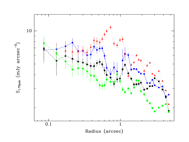
Figure 3: The observed surface brightness as a function of radius at 1.7$\mu m$ measured separately for each of the four image quadrants surrounding Sgr A^∗. The error bars shown in Figure 2 are the uncertainty in the mean at a given radius of these data. The colors for quadrants 1, 2, 3 and 4 are blue, red, black and green, respectively. The first quadrant is in the upper-left corner of the image (NE on the sky) and rotate around counterclockwise.

We also evaluated the systematic uncertainties in our results due to the measurement techniques, such as the star masking, the particular choice of aperture radii, and local variations in surface brightness due to the inherent distribution of individual stars around Sgr A^∗. For example, we compared the variations in surface brightness distributions within the four separate image quadrants surrounding Sgr A^∗. The resulting distributions are shown in Figure 3. We have used the uncertainty in the mean of these four measurements at a given radius as an uncertainty in the azimuthally-averaged results shown in Figure 2.

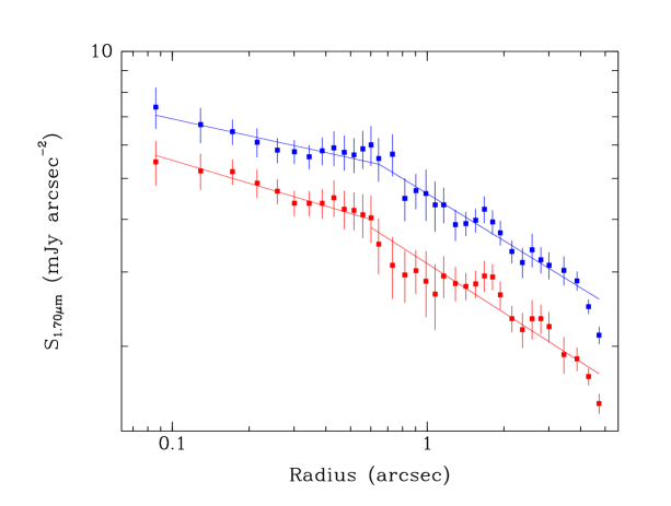
Figure 4: The observed surface brightness as a function of radius at 1.7$\mu m$ using the mean (upper) and median (lower) of the unmasked pixel values within each photometric annulus. The two curves has been offset vertically for clarity. The slopes for the two methods are identical to within the uncertainties.

We also compared results using different series of aperture radii, in order to determine if any bias is being introduced by the large variation in aperture area from the smallest to the largest apertures. Several different sets of aperture radii that used somewhat more balanced numbers of pixels per aperture all yielded the same overall profile shape, with the distinctive change in slope near r$\sim$0.6–0.8^′′ (as discussed in the following section). Finally, we also computed the surface brightness using the median signal within each annulus and compared it with the standard results that use the mean. As can be seen from the comparison shown in Figure 4, both methods yield the same slope in surface brightness distribution, to within the uncertainties of the slope fits.

3 Results and Discussion

Plots of the surface brightness of stars as a function of distance from Sgr A^∗ for all three bands have been presented in Figure 2, both with and without extinction corrections. Least-squares fits to the surface brightness distributions are also superimposed. The slope of the distribution in all three bands is significantly steeper at radii $>$  0.7^′′. In each band we determined weighted fits using a broken, two-part power law. The least-squares fits to the outer regions did not include the two outermost data points (r$>$4^′′) due to a systematic drop in surface brightness near that radius. Table 1 shows the parameters of the individual fits in each wavelength band. The fit parameters are quite consistent amongst the three bands. For radii $>$ 0.7^′′, the slope is a relatively steep $\beta=-0.34\pm 0.04$, where $\Sigma$ $\propto r^{\beta}$, and becomes flatter at smaller radii with $\beta=-0.13\pm 0.04$. We note that Sabha et al. (2010) have applied different methods of PSF subtraction to their AO data and have detected residual diffuse emission within 0.5^′′ of Sgr A^∗. These authors note a decrease in diffuse light away from Sgr A^∗ with $\beta=-0.20\pm$0.05 over a range in projected distance of 0.03–0.2^′′, which is consistent with that of our measurements within r$\sim$0.7^′′.

3.1 Artifical Star Clusters

In order to test whether the flattening of the surface brightness distribution at small radii could be an artifact of our measurement techniques, we applied the same measurements to artificial star clusters and compared the results. We used tasks in the IRAF artificial data (“artdata”) package to create the artificial clusters, using a NICMOS camera 1 PSF generated by the STScI program “Tiny Tim”. The task “starlist” was first used to generate a list of 2000 stars distributed over an x/y coordinate space of the same extent as our NICMOS images, with an $r^{-0.8}$ spatial distribution (corresponding to a space density of $r^{-1.8}$) and a power-law luminosity distribution. Ranges of artificial magnitudes were chosen to result in flux levels similar to those in the NICMOS images of Sgr A^∗. The “mkobjects” task was then used to produce an artificial image, using a NICMOS camera 1 PSF generated by the STScI program “Tiny Tim” to create suitable profiles at each of the positions in the star list, along with appropriate levels of Poisson and read noise. Ten separate artificial clusters were generated in this way, using different seeds for the random number generators that produce the star catalog.

Two images were produced for each of the ten artificial clusters, which allowed us to assess the effectiveness of the masking technique that we applied to the bright stars in the NICMOS images. We generated one image of each cluster that contained all the bright stars in the catalog produced by “starlist” and then applied masking to the bright stars over the same range of magnitudes as that in the NICMOS images. We also generated an image for each cluster that excluded the set of bright stars from the catalog, so that the bright stars did not appear in the images. We then measured the surface brightness distributions in each of the cluster images using the same technique as that applied to the NICMOS data. Figure 5 shows the results.

The upper set of points in Figure 5 shows the average surface brightness distribution for the ten artificial clusters that did not contain any of the bright stars. Similarly, the lower set of points corresponds to the data for the clusters in which the bright stars were masked out. The two sets of points have been offset from one another along the y-axis of the plot for the sake of clarity. The error bars indicate the standard deviation of the values amongst the ten simulations at each radius. The spread in data values is naturally somewhat larger for the clusters that had masking applied, due to the smaller number of data points used at each radius.

There are two important points to notice from these results. First, there is very little difference between the results derived from the masked images and the images that did not include the bright stars. The slopes of the least-squares fits are identical to within the fit uncertainties. This indicates that the masking technique that was applied to the NICMOS images is effective at removing the contributions of the bright stars near Sgr A^∗. Second, the surface brightness profiles of both versions of the artificial clusters are well-fit by a single power law, with very little deviation from the linear fit. In contrast to the measurements made from the NICMOS images of Sgr A^∗, there is no indication of a different slope for radii $<$ 0.7^′′. Hence the flattening of the Sgr A^∗ profile at small radii does not appear to be an artifact of the data or the measurement techniques.

Table 1: Parameters of the Fit in Three Bands

Band ($\mu$m)	Radii (′′)	Slope ($\beta\pm\sigma$)
1.70	$<0.7$	-0.13$\pm 0.04$
-	$0.7-4.7$	-0.34$\pm 0.04$
1.45	$<0.7$	-0.14$\pm 0.04$
-	$0.7-4.7$	-0.39$\pm 0.04$
1.90	$<0.7$	-0.15$\pm 0.07$
-	$0.7-4.7$	-0.31$\pm 0.04$

3.2 Flattening of the Surface Brightness Distribution

The flattening of the slope in the two-part fit is consistent with AO measurements (Schödel et al. 2007) in that the slope becomes steeper with increasing radii, with $\beta$=–0.13 for $r<0.7$^′′ and $\beta$=–0.34 for $r=0.7-4.7$^′′. The distribution of total light within 0.7^′′ has a similar slope, because the disks of massive stars are located beyond 0.8^′′. AO measurements show a flattening of the evolved faint stars after having identified and removed the contributions of B stars. To make both measurements consistent with each other, the NICMOS data must be contaminated by faint members of the S cluster within 1^′′ of Sgr A^∗. Alternatively, because we have sampled the diffuse stellar emission within the inner 1^′′ better than stellar counts from AO measurements, the NICMOS data includes the background light that may have not been detected or included in the AO results. To understand the origin of this discrepancy, we have converted the observed flux of 7.72 mJy from the region within 1^′′ of Sgr A^∗ and estimated an equivalent H-band magnitude, which is the band closest to our 1.7$\mu$m band, of 12.8. Using the observed $H-K$ color of  2 for a population of evolved stellar sources in the Galactic center region (Maness et al. 2007), we expect K=10.8 mag within 1^′′ of Sgr A^∗. This is equivalent to $\sim$76 stars of K=15.5 mag in the inner 1^′′. Number counts of stars within 1^′′ clearly show a smaller number of K=15.5 stars than this (e.g., Bartko et al. 2010; Buchholz et al. 2009), suggesting that this light comes from dwarf stars rather than the giants that would be detectable in the AO observations (see §3.3). The equivalent number of stars also exceeds the extrapolations of the luminosity functions based on the number counts, consistent with the excess being the integrated light from dwarves.

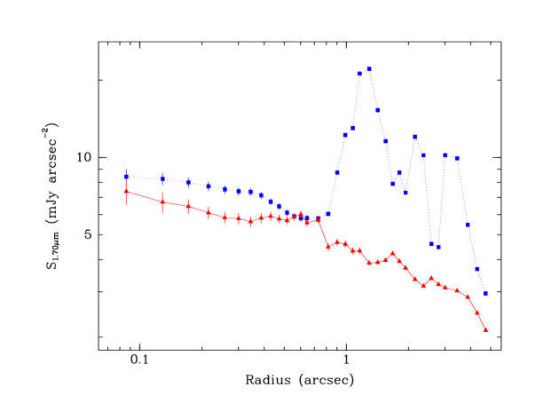
Figure 6: A comparison of the 1.7$\mu$m surface brightness distributions measured with (red) and without (blue) masking of the bright, young stars in the NICMOS image.

The measurements presented here also confirm that the sudden drop in the radial profile of starlight near r=0.8^′′ reported by Scoville et al. (2003) does not actually exist. Scoville et al. (2003) attempted to remove the contribution of massive stars by discarding the signal from the brightest 20% of the pixels in each photometric annulus around Sgr A^∗. This, however, produces a variable rejection threshold as a function of radius, depending on the maximum brightness of stars included in each annulus. Figure 6, which shows a comparison of the surface brightness distribution with and without rejection of the bright stars, shows the complexity and dominance of the light from bright stars outside 1^′′ radius. The bright stars (shown by the blue line in Figure 6) contribute a large amount of signal at $r>0.8$^′′, which produces an obvious bump in the distribution. The dip that was reported by Scoville et al. (2003) inside of r=0.8^′′ is in fact simply due to this peak in the number of bright stars just outside that radius, which was not completely removed from their measurements. If the bright stars are completely masked, the dip in the surface brightness near 0.8^′′ disappears, as shown in Figure 6.

3.3 Model Fitting

We have also fit our surface brightness distributions using a parametrized form of the three-dimensional luminosity density profile and projecting it onto the plane of the sky. We follow Merritt (2010) and adopt a spherically-symmetric luminosity-density profile for the stellar cluster, using

$$\rho_{L}(r)=\rho_{0}\left(\frac{r}{r_{0}}\right)^{-\gamma_{i}}\left[1+\left(\frac{r}{r_{0}}\right)^{\alpha}\right]^{(\gamma_{i}-\gamma)/\alpha}\,,$$ (1)

which behaves as $r^{-\gamma_{i}}$ for $r\ll r_{0}$, and $r^{-\gamma}$ for $r\gg r_{0}$, with $\alpha$ controlling the sharpness of the transition from the outer to inner power-law around $r_{0}$. We also follow Merritt (2010) in fixing $\alpha=4$ and, because our data do not extend to very large radius, impose $\gamma=1.8$ to follow previous determinations at large $r$. We integrate equation 1 along the line of sight to compute the surface brightness profile and adjust the parameters $n_{0}$, $r_{0}$, and $\gamma_{i}$, for each band, to minimize $\chi^{2}$.

Table 2: Fits to surface brightness profile

fit	$\rho_{0}$ 1.45$\mu$m	$\rho_{0}$ 1.70$\mu$m	$\rho_{0}$ 1.90$\mu$m	$r_{0}$	$\gamma_{i}$	$\chi^{2}/\textrm{d.f.}$
	(mJy arcsec-3)	(mJy arcsec-3)	(mJy arcsec-3)	(arcsec)
1.45 $\mu$m only	15.03	—	—	3.37	0.94	0.63
1.70 $\mu$m only	—	11.19	—	3.73	0.87	0.59
1.90 $\mu$m only	—	—	8.40	4.36	0.92	0.28
simultaneous	13.31	11.22	10.75	3.69	0.89	0.55
$\gamma_{i}=0.5$	28.10	23.97	22.66	2.36	0.50	0.94
$\gamma_{i}=1.25$	0.647	0.536	0.524	27.4	1.25	1.28
fixed $r_{0}$	6.23	5.24	5.04	6.00	1.06	0.73

Figure 7 and Table 2 compare individual profiles from NICMOS data in the 1.45, 1.7 and 1.9$\mu$m filters with simultaneous fits across all three bands, as shown in blue. For the individual fits, the values of $r_{0}$ and $\gamma_{i}$ increase with wavelength, which means that there is very little difference between the simultaneous fits and the 1.7$\mu$m fit, because the differences in the shapes at 1.45 and 1.9$\mu$m relative to that at 1.7$\mu$m tend to cancel. The reduced $\chi^{2}$ drops in moving between the separate fits for the 1.7, 1.45, and 1.9$\mu$m data simply because of the decrease in S/N between the bands. Overall, the values of reduced $\chi^{2}$ that we obtain are small, suggesting that the error bars may be overestimated. Therefore, we cannot use the magnitude of $\chi^{2}$ to reliably determine confidence limits for the model parameters. This limitation aside, the best fit to the data suggests that the stellar luminosity density profile flattens as $\sim r^{-0.9}$ within 3–4^′′ of Sgr A^∗. We do not find evidence for a decline in stellar density (i.e. negative values of $\gamma_{i}$) in the inner arcsecond, in contrast to the results of Do et al. (2009; see also Merritt 2010). The best-fit for an $r^{-0.5}$ inner profile, as shown with red short-dashed line, is only marginally consistent with the observed surface density profile.

Our values of $r_{0}$ are not very well determined as our data extend only to 5^′′ from Sgr A*. To assess this uncertainty we also consider a fit with $r_{0}$ fixed at 6^′′ (dashed blue curve in Fig. 7), consistent with the profiles found by Schödel et al. (2007) and Bartko et al. (2010). This yields $\gamma_{i}=1.06$ and a slightly larger value of the $\chi^{2}$ per degree of freedom, and so we conclude that $\gamma_{i}$ may be larger than the 0.89 we obtain when $r_{0}$ is allowed to be adjusted.

Converting our measured diffuse light profile to a stellar mass profile is not straightforward. The intrinsic colors inferred from the ratios of the $\rho_{0}$ values derived from simultaneously fitting the profiles in the three NICMOS bands are consistent with either giant stars with spectral types of G4 III – K0 III, or K0–K2 dwarfs. The former would be bright enough (extinction-corrected H$\lower 1.72218pt\hbox{$\;\buildrel<\over{\scriptstyle\sim}\;$}13$) to be detected as point sources, so it is reasonable to assume that the light is dominated by K0 dwarfs, which would have an extinction-corrected $H\approx 18.7$ (corresponding to an F170M flux of about $4\times 10^{-5}$ Jy) and mass $\approx 0.8$M_⊙ (e.g. Binney & Merrifield 2000). The corresponding conversion factor between F170M flux and stellar mass is then $2.05\times 10^{4}\,\mathrm{M}_{\odot}\mathrm{Jy}^{-1}$, and the luminosity density at 1.7µm implies that the mass enclosed within $r\lower 1.72218pt\hbox{$\;\buildrel<\over{\scriptstyle\sim}\;$}0.1$ pc is $\approx 3.2\times 10^{4}$ M${}_{\odot}(r/0.1\,\mathrm{pc})^{2.1}$. This is in reasonable agreement with Schödel et al (2009), who used the diffuse light at 10^′′ in their $K_{s}$ band observations, the radial profile derived from counts of late-type stars, and a solar K-band luminosity-to-mass ratio to find $M(r)\approx 1.9\times 10^{4}\,\mathrm{M}_{\odot}(r/0.1\,\mathrm{pc})^{1.8}$ for $r\lower 1.72218pt\hbox{$\;\buildrel<\over{\scriptstyle\sim}\;$}0.8\,$pc. Adjusting Schödel et al’s $A_{K}=3.3$ mag to our adopted $2.42$ mag decreases this mass estimate by a factor of 0.44, yielding $0.85\times 10^{4}\,\mathrm{M}_{\odot}$ enclosed within 0.1 pc. For comparison, if we also assume that the diffuse light was dominated by G2 dwarfs, (extinction-corrected $H\approx 17.9$), our estimate of the stellar mass enclosed within 0.1 pc is $2.3\times 10^{4}$ M_⊙. These masses are all consistent with the analysis of proper motions measurements, which indicate a similar mass enclosed near Sgr A^∗ (Schödel et al. 2009). Morris (1993) claims the possibility of several 10⁵ $M_{\odot}$of stellar mass black holes in the innermost tenths of parsec of Sgr A*. Our analysis does not support the evidence for such a population of stellar remnants close to Sgr A*.

Our measurement of the surface brightness within a 10^′′ field centered on Sgr A^∗ is consistent with an $r^{-0.9}$ luminosity density profile in the innermost 0.1 pc, similar to the $r^{-1.12}$ power law inferred by Schödel et al. (2009) from counts of late-type stars. For such a flat inner profile, the surface brightness is insensitive to reductions in the luminosity density within 0.01 pc of Sgr A*, because the surface brightness is dominated by the luminosity density at larger radii. Nevertheless, our analysis finds no evidence of reduction in the diffuse light distribution within 0.1 pc. In contrast, Buchholz et al. (2009) found a reduction in the number counts of starts brighter than 15.5 K magnitude in the inner 0.1 parsec. These are marginally consistent with an $r^{-1}$ profile (Merritt 2010), but may suggest preferential removal of giants.

One mechanism that can destroy the $r^{-1.75}$ cusp expected from a relaxed system of stars near a supermassive black hole (Bahcall & Wolf 1976) is mass segregation, with black holes tending to settle towards the center while boosting stars to larger radii (e.g. Preto & Amaro-Seoane 2010). The resulting inner power law, $\gamma_{i}\approx-1.25$, is still too steep to be consistent with our data, as shown by the corresponding surface-density profiles (long-dashed red curves) in Figure 7. An alternative is that some process has removed the lowest energy stars near the center, which results in a shallower power law in the core, down to a limiting value (for isotropic velocity distributions) of $\gamma_{i}=0.5$, that can survive for several Gyr (Merritt 2010). This limiting value of $\gamma_{i}$ appears to be marginally consistent with our surface brightness profile, and larger values are more consistent with our measured profile. Another process that could slow down the two-body relaxation time scale is the presence of extended clouds from which the massive stars formed during the history of star formation in the nuclear star cluster. Future numerical simulations should include the effects of star forming gas clouds in the evolution of stellar clusters that surround massive black holes.

Acknowledgments: We thank the referee for many excellent and useful comments. This work is partially supported by grants AST-0807400 from the National Science Foundation and DP0986386 from the Australian Research Council.

Figure 2: (a) Left The observed surface brightness as a function of radius in the 3 NICMOS bands. A two-part fit is superimposed on the radial profile with parameters as shown in Table 1. (b) Right Same as (a) except that the fluxes are extinction corrected using $A_{1.45\mu m}=6.07$, $A_{1.7\mu m}=4.34$, and $A_{1.9\mu m}=3.46$.

Figure 5: Averaged profiles and fits for the 10 artificial clusters. The upper line, with square markers, is the data for the clusters that did not have the bright stars included in the images. The lower line, with triangular markers, is for the clusters that had the brights stars masked. The two sets of data have been artificially separated along the y-axis for clarity. Error bars are the standard deviation amongst the 10 clusters at each radius.

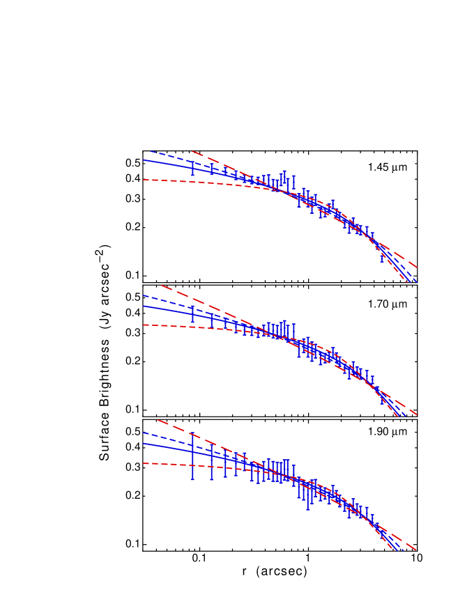
Figure 7: Sample fits to the HST data. Blue solid curves show the best simultaneous fit across all 3 bands. Red short-dashed and long-dashed curves show the best simultaneous fits obtained when $\gamma_{i}$ is fixed at 0.5 or 1.25, respectively (see text). Blue short-dashed curve shows the simultaneous fit when $r_{0}$ is fixed at 6” (see text)

References

- Alexander (2005) Alexander, T. 2005, Physics Reports, 419, 65
- Alexander (2005) Alexander, T. 2007 in ”2007 STScI spring symposium: Black Holes”, eds, M. Livio & A. M. Koekemoer, Cambridge University Press (arXiv:0708.0688)
- Bahcall & Wolf (1976) Bahcall, J. N. & Wolf, R. A. 1976, ApJ, 209, 214
- Bahcall & Wolf (1976) Bahcall, J. N. & Wolf, R. A. 1977, ApJ, 216, 883
- Bailey & Davis (1999) Bailey, V.C. & Davies, M.B. 1999, MNRAS, 308, 257
- Bartko et al. (2010) Bartko, H. et al. 2010, ApJ, 708, 834
- Binney and Merrifield (2000) Binney, J. & Merrifield, M. 2000, in Galactic Astronomy, Princeton University Press
- Buchholz et al. (2009) Buchholz, R. M., Schödel, R. & Eckart, A. 2009, A&A, 499, 483
- Becklin & Neuhebauer (1968) Becklin, E.E. & Neugebauer, G. 1968, ApJ, 151, 145
- Catchpole, Whitelock and Glass (1990) Catchpole, R. M.; Whitelock, P. A.; Glass, I. S. 1990, MNRAS, 247, 479
- Do et al. (2009) Do, T. et al. 2009, ApJ, 703, 1323
- Eckart et al. (1993) Eckart, A., Genzel, R., Hofmann, R., Sams, B. J., and Tacconi-Garman, L. E., 1993, ApJ, 407, L77
- Fritz et al. (2011) Fritz, T. K., Gillessen, S., Dodds-Eden, K., Lutz, D., Genzel, R. et al. 2011, ApJ, in press (2011arXiv1105.2822)
- Genzel et al. (2010) Genzel, R., Eisenhauer, F., and Gillessen, S. 2010, Reviews of Modern Physics, 82, 3121,
- Genzel et al. (1996) Genzel, R., Thatte, N., Krabbe, A., Kroker, H., & Tacconi-Garman, L.E. 1996, ApJ, 472, 153
- Genzel et al. (2003) Genzel, R. et al. 2003, APJ, 594, 812
- Ghez et al. (2008) Ghez, A. et al. 2008, ApJ, 689, 1044
- Gillessen et al. (2009) Gillessen, S. et al. 2009, ApJ, 692, 1075
- Haller et al. (2000) Haller, J. W., Rieke, M. J., Rieke, G. H., Tamblyn, P., Close, L., and Melia, F., 1996, ApJ, 468, 955
- Hansen & Milosavljevic (2003) Hansen B.M.S. & Milosavljevic, M. 2003, ApJ, 593, L77
- Hopman & Alecxander (2006) Hopman, C. & Alexander, T. 2006 ApJ, 645, 1152
- Launhardt et al. (2010) Launhardt, R., Zylka, R.,& Mezger, P. G. 2002, A&A, 384, 112,
- McGinn et al. (1989) McGinn, M. T., Sellgren, K., Becklin, E. E., and Hall, D. N. B. 1989, ApJ, 338,824
- Maness et al. (2010) Maness, H. et al. 2007, ApJ, 669, 1024
- Merritt (2010) Merritt, D. 2010, ApJ, 718, 739
- Morris (1993) Morris, M. 1993, ApJ, 408, 496
- Paumard et al. (2006) Paumard, T. 2006, ApJ, 643, 1011
- Peebles (1972) Peebles, P. 1972, ApJ, 178, 371
- Preto et al. (2010) Preto, M. & Amaro-Seoane, P. 2010, ApJ, 708, L42
- Rieke & Rieke (1994) Rieke, G. H., & Rieke, M. J. 1994, in The Nuclei of Normal Galaxies, ed. R. Genzel & A. I. Harris (Dordrecht: Kluwer), 283
- Reid & Brunthaler (2004) Reid, M. J. and Brunthaler, A. 2004, ApJ, 616, 872
- Sabha et al. (2010) Sabha, N., Witzel, G., Eckart, A., Buchholz, R. M., Bremer, et al. 2010, A&A,512, A2
- Schödel et al. (2007) Schödel, R., Eckart, A., Alexander, T., Merritt, D., Genzel, R., Sternberg, A., Meyer, L., Kul, F., Moultaka, J., Ott, T., and Straubmeier, C. 2007, A&A, 469, 125
- Schödel et al. (2009) Schödel, R., Merritt, D., and Eckart, A. 2009, A&A 502, 91
- Scolville et al. (2003) Scoville, N. Z., Stolovy, S.R., Rieke, M., Christopher, M. & Yusef-Zadeh, F. 2003, ApJ, 594, 294
- Sellgren et al. (1990) Sellgren, K., McGinn, M. T., Becklin, E. E., & Hall, D. N. B. 1990, ApJ, 359, 112
- Trippe (2008) Trippe, S., Gillessen, S., Gerhard, O. E., Bartko, H., Fritz, T. K., Maness, H. L., Eisenhauer, F., Martins, F., Ott, T., Dodds-Eden, K., and Genzel, R. , 2008, A&A, 492, 419 Yu, Q. & Tremaine, S. 2003, ApJ, 599, 1129
- Yu & Tremaine (2003) Yu, Q. & Tremaine, S. 2003, ApJ, 599, 1129