Dissolution of traffic jam via additional local interactions

Abstract

We use a cellular automata approach to numerically investigate traffic flow patterns on a single lane. The free-flow phase (F), the synchronized phase (S), and the jam phase (J) are observed and the transitions among them are studied as the vehicular density $\rho$ is slowly varied. If $\rho$ is decreased from well inside the J phase, the flux $\Phi$ follows the lower branch of the hysteresis loop, implying that the adiabatic decrease of $\rho$ is not an efficient way to put the system back into S or F phases. We propose a simple way to help the system to escape out of J phase, which is based on the local information of the velocities of downstream vehicles.

Since 1990s, traffic phenomena have drawn much attention amongst physicists review . Pure theoretical interest of the study of the traffic problem originates from its variety of fascinating dynamic emergent behaviors HK-empirical , like the phase transitions between different dynamical states, the existence of hysteresis behavior, and the historic dependence of traffic flow, to name a few. Recently, there has been a growing consensus on the existences of three different dynamic phases: when the vehicular density $\rho$ is small enough, the system first stays in the free-flow (F) phase in which vehicles can have the maximum speed allowed, and thus the flux $\Phi$ is linearly proportional to $\rho$. As $\rho$ is increased, the speeds of vehicles are synchronized (S phase) to each other, without having stop-and-go motion, and then eventually the jam (J) phase arises beyond some value of $\rho$.

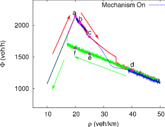
Figure 1: (Color online) Fundamental diagram: the flux $\Phi$ versus the vehicular density $\rho$ shows a hysteresis behavior. As $\rho$ is increased from the free-flow (F) phase (a), $\Phi$ follows the upper branch of the curve, passing the synchronized (S) phase (b and c), and the jam (J) phase (d). When started from the J phase (d), $\Phi$ follows the lower branch of the curve, passing the points e and f (both are in J phase, see Fig. 2). The dotted blue curve in the middle is obtained when our method of dissolution of the jam by using an additional interaction is turned on.

The cellular automata (CA) model proposed by Kerner et al. (KKW) KKW to explain the three traffic phases, has been recently applied for multilane roads and compared with single vehicle data measured on American highway kk2009 . Knospe et. al. knospe extended Nagel-Schreckenberg model NaSch to include the anticipation effect and the reduced acceleration capabilities, and a further extension was made by Jiang and Wu jiang with the difference of sensitivities between stopped and moving cars taken into account. Davis davis used the modified optimal velocity model and also produced the synchronized flow phase, but with unrealistic speed of upstream front. In Ref. hklee , realistic assumptions of the limited deceleration capability and human overreaction has been used as important ingredients of the CA model. Similar ideas of the limited decelerating capability and cautious driving when congested have been adopted in Ref. yang , in which a further improvement was made by letting the maximum speed be dependent on headway distance to incorporate the idea of the comfortable driving. A CA model with the similar deceleration limitation but without the slow-to-start effect has been proposed, which again reproduced the three traffic phases and discontinuous transitions between them jin , which in turn suggests that the slow-to-start effect is not a cause but a result of the transition to the wide-moving jam. In Ref. xgli , an attempt to interpret the traffic flow in the viewpoint of the complex network of traffic states was made. Very recently, the emergence of a jam without bottlenecks has been observed experimentally sugiyama , which clearly indicates that the traffic jam is a collective phenomenon resulting from interactions between vehicles. In the present paper, we follow the same line of reasoning and propose that one can use an additional local interaction to dissolve the traffic jam.

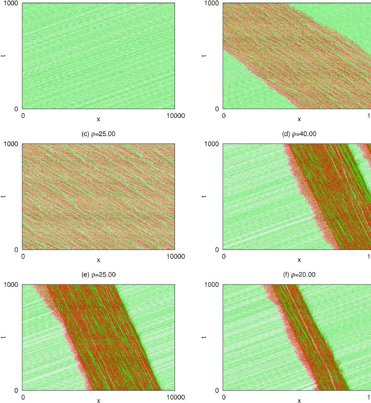
Figure 2: (Color online) Spatio-temporal ($x$,$t$) patterns of traffic flows at points a - f in Fig. 1. Dots with bright and the dark colors (green and red online, respectively) represent vehicles at optimistic and defensive states. As the vehicular density $\rho$ is increased (see Fig. 1), transitions occur from (a) the F phase to (c) the homogeneous S phase and then to (d) the J phase. Between the F and the homogeneous S phase, the inhomogeneous S phase in (b) is observed. As $\rho$ is slowly decreased, the system does not escape out of the J phase [compare (e) and (c), and (f) and (a), respectively].

The main purpose of the present work is not to propose another traffic model, but to study how the traffic jam can be dissolved through the use of the local information of car traffic. In this regard, we use the same CA model as in Ref. hklee , which has the mechanical restriction (implemented as limited acceleration and deceleration capabilities) and the human overreaction as two important ingredients of the model. Throughout the present study, discretized one unit of time (distance) amounts to $\Delta t=$1 s ($\Delta x=$1.5 m), and $x_{n}^{t}(v_{n}^{t})$ denotes the position (the velocity) of the $n$th vehicle at time $t$. The human driving behavior is described by the two-state variable $\gamma_{n}^{t}$, which is set to $\gamma_{n}^{t}=0$ for $v_{n}^{t}\leq v_{n+1}^{t}\leq v_{n+2}^{t}$. We also assign $\gamma_{n}^{t}=0$ for $v_{n+2}^{t}\geq v_{\rm max}-1$ with the speed limit $v_{\rm max}$. If neither condition above is satisfied, we set $\gamma_{n}^{t}=1$ instead. In words, if the speed is successively nondecreasing in the downstream direction the driver expects that the traffic condition is improving. She can also be optimistic when the second leading vehicle is fast enough. The variable $\gamma$ is not quenched but can change in time, and describes the driving behavior of each driver. It is to be noted that both $\gamma=0$ and $\gamma=1$ represent human overreaction and only the type of overreaction is different (optimistic and defensive).

We sketch here only the basic ideas of the model in Ref. hklee : a driver in the optimistic (defensive) state with $\gamma=0(1)$ leaves less (more) distance to the leading vehicle than that required for her safety. In comparison, an optimistic driver tries to avoid a collision only up to some time steps. By introducing optimistic and defensive behaviors, human factor is modeled as an overreaction to the local traffic condition. It is also assumed that vehicles can neither exceed the speed limit $v_{\rm max}=20$ (corresponding to 108 km/h), nor drive in the opposite direction ($v<0$). As another important ingredient of the model, each vehicle can decrease their velocity stochastically, to implement the random driving behavior in reality. All the parameter values are set identical to those in Ref. hklee to mimic empirical observations. In Ref. sugiyama , the critical vehicular density separating the free-flow phase the congested flow phase for the experimental setup of circularly moving cars was found to be about 25 vehicles/km as observed in real highway traffic, and the speed of the downstream jam front was measured as 20km/h. In the present study, for example, the downstream speed of the wide moving jam is found to be 18.4km/h, similar to the empirical measurement.

We first report our simulation result footnote for the fundamental diagram. We use the single lane of the size $L=$40 000 (corresponding to 60 km) under the periodic boundary condition. As an initial condition we uniformly distribute $N=600$ vehicles [$\rho=10$ veh/km] and run the simulation by using the model in Ref. hklee . In order to neglect transient behaviors, we ignore the first $T$ time steps and measure the average speed $v_{\rm avg}\equiv(1/T)\sum_{t=T+1}^{2T}v(t)$ for another $T$ steps, where the spatial average $v(t)\equiv(1/N)\sum_{n=1}^{N}v_{n}^{t}$. The traffic flux is then computed by $\Phi\equiv\rho v_{\rm avg}$. We confirm that $T=$ 30 000 is long enough to ensure that the system approaches the steady state. The slow increase and the decrease of $\rho$ are implemented as follows: in order to disturb the flow as little as possible, the addition of a single vehicle is done at the position where the distance between two cars ($x_{n+1}-x_{n}$) is maximum. When a car is removed from the road, it is done for the slowest car, in order to make the jam dissolve more easily.

Figure 1 exhibits the (global) fundamental diagram, the flux $\Phi$ versus the vehicular density $\rho$. The upper branch of the curve is obtained when $\rho$ is slowly increased. When $\rho=50$(veh/km) is approached from below, we begin to decrease $\rho$ as described above. The dotted blue curve marked as ”Mechanism On” in Fig. 1 will be explained below. As is well-known, the fundamental diagram exhibits hysteresis behavior: $\Phi$ follows different curves as $\rho$ is increased and decreased. The existence of the hysteresis loop indicates that once the traffic jam is formed, it is quite difficult to dissolve the jam unless the vehicular density is significantly decreased. On the other hand, if we decrease $\rho$ when the system is at point c in Fig. 1, we confirm that the system can easily go back to the F phase. In other words, in the present model, there is no hysteresis behavior between the F phase and the S phase, which in turn indicates that the transition between S and F is not discontinuous in our study. In comparison, some of existing CA model studies have produced a continuous F-S transition jiang ; gao as in the present work, while others supported the discontinuous transition jiang2 .

For better understanding of the characteristics of the three different phases, the spatio-temporal traffic patterns are displayed in Fig. 2: each panel corresponds to six different points (a-f) in the fundamental diagram (Fig. 1). An advantage of the traffic model in Ref. hklee is that we can easily see the connection between driving behavior and the traffic flow. In the F phase [a in Fig. 1 and Fig. 2(a)], almost all drivers become optimistic and drive at the maximum speed allowed. As $\rho$ is increased, the inhomogeneous S phase (b) is clearly observed between (a) the F and (c) the homogeneous S phases. A further increase of $\rho$ eventually results in (d) the J phase. Interestingly, we observe that the downstream front of the jam and the downstream front of the synchronized region move at different speeds, as can be compared in Figs. 2(b) and (d) footnote2 . We emphasize that the traffic flow patterns in Fig. 2 are obtained after long periods: under the periodic boundary condition adopted in the present study, once the jamming occurs, it is not spontaneously dissolved either to the F phase [from (f) to (a)] or to the S phase [from (e) to (c)]. The measured speed ($\approx$ 50 km/h) of the downstream front of the synchronized region in Fig. 2(b) is much higher than the corresponding speed ($\approx$ 18.4 km/h) for the jammed region in Fig. 2(e) and (f). In comparison, the improved Kerner’s three-phase model in Ref. jiang3 has produced a realistic speed (5 cells per time unit corresponding to 8.5km/h) of the downstream front of the synchronized flow, while in Fig. 3 of Ref.jin the corresponding speed is measured to be roughly about 32km/h. We remark that the somehow unrealistically high speed of the downstream front of the synchronized flow in Fig. 2(b) could be an artifact of the present model. Likewise, the absence of the hysteresis behavior around S-F transition could also be model dependent.

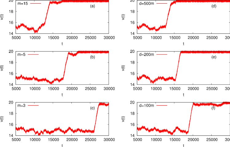
Figure 3: (Color online) The average speed $v(t)$ versus the time $t$. We start from the J phase (at f in Figs. 1 and 2), and turn on our jam dissolving mechanism (see text) at $t=5000$. (a)-(c) The first method based on the speed of the $m$-th leading vehicle. (d)-(f) The second method based on the speed of the vehicle at the geographic distance $d$.

The main objective of this study is to suggest a simple way to dissolve the traffic jam within the limitation of the present CA model. If strong enforcement by the central authority is allowed, the most efficient way to have maximum traffic flow is to directly control the vehicular density $\rho$ so that traffic flow is tuned toward the point a in Fig. 1. In this iron-fist solution, more cars are allowed to enter the road if $\rho<\rho_{c}\approx 20$(veh/km), while all the entrances are blocked if $\rho>\rho_{c}$. Although not realistic, this centralized way of maximizing traffic flow could be a very efficient way thanks to the absence of the hysteresis behavior between the F and the S phases. In other words, although the central authority fails to detect the maximum-flow condition $\rho=\rho_{c}$ and thus the synchronized flow already starts, a simple reduction of $\rho$ will put the traffic back to the free-flow state. In the real-world traffic, however, it is not plausible that drivers are willing to accept the centralized control. We believe that the above consideration raises an interesting issue in the game theoretic situation: near $\rho=\rho_{c}$, the flow is maximum and every driver will complain much if she is not allowed to enter the road which her leading vehicle just entered in a few seconds earlier. For her own sake, she is better off entering the road against the will of the central authority. However, in the public perspective, the overall traffic flow becomes worse by allowing her to get in. A similar situation has been termed as the price of anarchy in the study of urban car traffic poa .

It is to be noted that in real traffic situations, feedback control of traffic flux at ramps is better suited to dissolve the traffic jam than the control of the global average vehicular density. The spatial inhomogeneity and the unavoidable time lag between the start of the control and the system’s response require adaptive control on ramps. In this regard, ”ramp-metering” has already been well studied and applied in real highway systems ramp .

We suggest below a noncentralized way to dissolve the traffic jam which is based on local traffic information. Traffic flow can be of course improved by building a new road. However, the construction of new roads is not a practical alternative anymore in most countries acc . Accordingly, a recent focus towards better traffic flow has been made regarding how we can use existing roads in a more intelligent way. One of the promising directions for achieving better traffic flow is by using the so-called adaptive cruise control acc ; HK-acc2 . The basic idea behind this is that each car can be equipped with a detector which senses local traffic information and sends it to nearby cars. This gathered information can then be used to decide a driving strategy. In the same spirit, we propose below a jam dissolving mechanism which is based on downstream traffic information.

The robustness of the jam phase indicates that the incoming flux to the jam is not smaller than the outgoing flux. Accordingly, if an appropriate softening of the myopic behavior of jam-approaching drivers is made, it could reduce the incoming flux, resulting in the eventual dissolution of the jam. From this reasoning, we propose a simple way to dissolve the jam: if a vehicle is approaching the upstream jam front, the driving behavior becomes defensive. In this regard, the use of the model in Ref. hklee has a great benefit since the model already contains the dynamic variable $\gamma$ which describes the driving behaviors. Accordingly, our method is written as

• If the $m$th leading vehicle has speed lower than the threshold value $v_{th}$, (i.e., if $v_{n+m}^{t}<v_{th}$), the driver becomes defensive ($\gamma_{n}^{t}=1$).

In the broad range of $m$ and $v_{th}$ we indeed observe that the traffic jam is dissolved. We then try to optimize the values of $m$ and $v_{th}$ to make the dissolution of the jam happen as quickly as possible. As a result, we find that when $v_{th}=8(\approx 43$ km/h) and $10\leq m\leq 30$ the jam is dissolved faster than the use of other values of $v_{th}$ and $m$. In Fig. 3(a)-(c), we display the jam dissolving behavior for various values of $m$: even at $m=3$ the jam is found to dissolve eventually, as shown in Fig. 3(c). It is noteworthy that the congested traffic state is characterized by $v<$40 km/h in Ref. acc , similar to our optimized value of $v_{th}$. We also use a modified version of our method in which the geographic distance $d$ to the downstream preceding vehicle is used instead of $m$: If the farthest vehicle in the downstream direction at a distance shorter than $d$ has a speed lower than $v_{th}$, $\gamma$ is set to one (defensive driving). We find that the jam is dissolved in a broad range of $d$ for $d\gtrsim 50$ corresponding to $d\gtrsim 75$ m [see Fig. 3(d)-(f)]. We also observe that if the fraction of vehicles with our method turned on is larger than about 80%, the jam is eventually dissolved for both types of our methods.

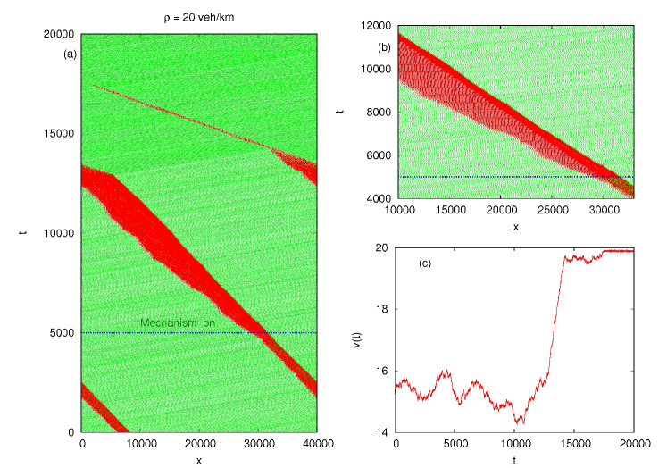
Figure 4: (Color online) (a) Spatio-temporal ($x$,$t$) pattern of the traffic flow starting from the J phase at point f in Figs. 1 and 2. After the jam dissolving mechanism proposed in this study is turned on at $t=$5 000, more drivers become defensive (red dots) in the intermediate times, and eventually the traffic jam is dissolved for all drivers become optimistic (green dots). (b) The expansion of a part of (a) to show more clearly that the jammed region becomes narrower after $t=$ 5000. (c) The spatial average speed $v(t)$ versus time $t$.

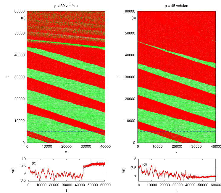
Figure 5: (Color online) Spatio-temporal ($x$,$t$) pattern of the traffic flow starting from the J phase at (a) $\rho=30$ and (c) $\rho=45$. The average velocity $v(t)$ as a function of time $t$ for the corresponding spatio-temporal pattern is also shown in (b) and (d). It is to be noted that at $\rho=30$, our jam dissolving mechanism improves the flow, while at $\rho=45$ it makes the flow worse (see Fig. 1).

Figure 4 exhibits the dissolution of the jam in the spatio-temporal plot ($x$-$t$) [(a) and (b)], and (c) the spatial average $v(t)$ as a function of time $t$, at $\rho=20.0$(veh/km). The initial state at $t=0$ is obtained from the long-time simulation at point f in Figs. 1 and 2, and the mechanism explained above is on at $t=$5 000 with the parameters $m=15$ and $v_{th}=8$. It is clearly seen that as time goes on, more and more jam-approaching drivers become defensive [Fig. 4(a)], and the jammed region with higher local density becomes narrower [Fig. 4(b)], as the upstream jam front eventually catches up the downstream jam front at $t\sim 14000$ [Fig. 4(a)]. Interestingly, a narrow track of defensive drivers persists for a quite long time, until all drivers become optimistic at around $t=$ 18 000. In Fig. 1, we also include the curve when our method of using additional downstream traffic information is turned on at all times. The key observations in Fig. 1 are as follows: (i) The hysteresis behavior disappears and thus increase and decrease of $\rho$ result in the same curve in the fundamental diagram. (ii) The use of our method greatly improves the traffic flow in a broad range of vehicular densities for $\rho\lesssim 26$, and effectively removes the jam phase in the lower branch. (iii) When $26\lesssim\rho\lesssim 31$, our method still helps but the traffic flow is worse than the upper branch without it. (iv) Interestingly, when $\rho\gtrsim 31$, the traffic flow with our method on is worse than the jam phase without it. (v) However, the jam that is robust in the broad range of $20\leq\rho\leq 30$ is efficiently dissolved by applying our simple method, which leads to a considerable flux increase compared to that of the jam phase in this density region.

For comparisons, we also display in Fig. 5 the spatio-temporal patterns and the average velocities versus time at $\rho=30$ [(a) and (b)], and $\rho=45$ [(c) and (d)], respectively. The mechanism is turned on at $t=$ 5 000 as in Fig. 4. At $\rho=30$, the congested region eventually spreads out and the average velocity in the steady state becomes larger than the value at the lower branch in Fig. 1 [see Fig. 5(b)]. In contrast, when the vehicular density is too high as in Fig. 5(c), the steady state value of the average velocity is smaller than the one with the mechanism off [see Fig. 5(d) and (iv) above].

In summary, we have used the single-lane traffic model proposed in Ref. hklee to study the nature of three traffic phases. As the vehicular density is slowly increased and decreased, hysteresis behavior is observed in the fundamental diagram for the flux and the density. Within the limitations of the used CA model, we propose a simple method to dissolve the jam, in which driving behavior is forced to become defensive if the leading vehicle a few cars ahead is dangerously slow. We believe that the main conclusion of jam dissolution via slowing down the jam-approaching vehicles by informing them of the speeds of leading vehicles could be general. However, the validity of our results needs to be checked more carefully in further studies. Our proposed mechanism dissolves the jam since it reduces the inflow without altering the outflow from the jam. Combined with the complementary method of increasing the outflow by using automated cruise control, the elimination of the jam can be made more effective.

B.J.K. was supported by Basic Science Research Program through the National Research Foundation of Korea (NRF) funded by the Ministry of Education, Science and Technology (2010-0008758), and H.K.L by grant (07-innovations in techniques A01) from the National Transportation Core Technology Program funded by Ministry of Land, Transport and Maritime Affairs of Korean government.

References

- (1) For reviews, see, e.g., D. Helbing, Rev. Mod. Phys. 73 (2001) 1067; D. Chowdhury, L. Santen, A. Schadschneider, Phys. Rep. 329 (2000) 199; T. Nagatani, Rep. Prog. Phys. 65 (2002) 1331.
- (2) I. Treiterer and J. A. Myers, in Proceedings of the 6th International Symposium on Transportation and Traffic Theory, edited by D. J. Buckley (Elsevier, New York, 1974); M. Koshi, M. Iwasaki, and I. Ohkura, in Proceedings of the Eighth International Symposium on Transportation and Traffic Flow, edited by V. F. Hurdle, E. Hauer, and G. N. Stewart (University of Toronto Press, Toronto, 1983).
- (3) B.S. Kerner, S.L. Klenov, and D.E. Wolf, J. Phys. A 35 (2002) 9971.
- (4) See, e.g., B.S. Kerner and S.L. Klenov, Phys. Rev. E 80 (2009) 056101, and references therein.
- (5) W. Knospe, L. Santen, A. Schadschneider, and M. Schreckenberg, J. Phys. A 33 (2000) L477.
- (6) K. Nagel and M. Schreckenberg, J. Phys. I 2 (1992) 2221.
- (7) R. Jiang and Q.-S. Wu, J. Phys. A 36 (2003) 381.
- (8) L.C. Davis, Phys. Rev. E 69 (2004) 016108.
- (9) H.K. Lee, R. Barlovic, M. Schreckenberg, and D. Kim, Phys. Rev. Lett. 92 (2004) 238702.
- (10) M.-L. Yang, Y.-G. Liu, Z.-S. You, Chin. Phys. Lett. 24 (2007) 2910.
- (11) C.-J. Jin, W. Wang, R. Jiang, and K. Gao, J. Stat. Mech. P03018 (2010).
- (12) X.-G. Li, Z.-Y. Gao, K.-P. Li, and X.-M. Zhao, Phys. Rev. E 76 (2007) 016110.
- (13) Y. Sugiyama, M. Fukui, M. Kikuchi, K. Hasebe, A. Nakayama, K. Nishinari, S. Tadaki, and S. Yukawa, New J. Phys. 10 (2008) 033001.
- (14) A Java Applet of the model can be found at http://statphys.skku.ac.kr/Applet/traffic.html.
- (15) K. Gao, R. Jiang, S.-X. Hu, B.-H. Wang, and Q.-S. Wu, Phys. Rev. E 76 (2007) 026105.
- (16) R. Jiang and Q.-S. Wu, Eur. Phys. J. B 46 (2005) 581.
- (17) When the ringroad system (or the road with the periodic boundary condition) is in the steady state, the upstream and the downstream fronts move at the same speed. In reality, the speed of the upstream front depends on the local influx of vehicles at the front and thus the speed of the downstream front is more fundamental quantity.
- (18) R. Jiang and Q.-S. Wu, Phys. Rev. E 72 (2005) 067103.
- (19) H. Youn, M.T. Gastner, and H. Jeong, Phys. Rev. Lett. 101 (2008) 128701.
- (20) M. Papageorgiou, Proc. 2000 IEEE Intelligent Transportation System Conf., pp 228.
- (21) Kesting, M. Treiber, M. Schönhof, and D. Helbing, Transportation Research Part C 16 (2008) 668.
- (22) L. C. Davis, Phys. Rev. E 69 (2004) 066110; B.S. Kerner, The Physics of Traffic (Springer, Berlin, 2004).