Multiplicity of supercritical fronts for reaction-diffusion equations in cylinders

Abstract

We study multiplicity of the supercritical traveling front solutions for scalar reaction-diffusion equations in infinite cylinders which invade a linearly unstable equilibrium. These equations are known to possess traveling wave solutions connecting an unstable equilibrium to the closest stable equilibrium for all speeds exceeding a critical value. We show that these are, in fact, the only traveling front solutions in the considered problems for sufficiently large speeds. In addition, we show that other traveling fronts connecting to the unstable equilibrium may exist in a certain range of the wave speed. These results are obtained with the help of a variational characterization of such solutions.

1 Introduction

Front propagation is a ubiquitous feature of many reaction-diffusion systems in physics, chemistry and biology [1, 2, 3, 4, 5, 6]. A question of particular interest that arises in a number of applications is related to fronts that invade an unstable equilibrium (for a review, see [7]). One of the well-known examples of such a system is given by a scalar reaction-diffusion equation in a cylindrical domain:

$$u_{t}=\Delta u+f(u,y).$$ (1.1)

Here $u=u(x,t)\in\mathbb{R}$ is the dependent variable, $x\in\Sigma\subset\mathbb{R}^{n}$ is a point in a cylindrical domain $\Sigma=\Omega\times\mathbb{R}$, whose cross-section $\Omega\subset\mathbb{R}^{n-1}$ is a bounded domain with the boundary of class $C^{2}$ (not necessarily simply-connected), and $t\in\mathbb{[}0,+\infty)$ is time. We will often write $x=(y,z)\in\Sigma$, where $y\in\Omega$ is the coordinate on the cylinder cross-section and $z\in\mathbb{R}$ is the coordinate along the cylinder axis. The function $f:\mathbb{R}\times\Omega\to\mathbb{R}$ is a nonlinear reaction term. On different connected portions of the boundary we assume either Dirichlet or Neumann boundary conditions (see [8] for the motivation of this particular choice of boundary conditions)

$$u\bigl{|}_{\partial\Sigma_{\pm}}=0,\qquad\nu\cdot\nabla u\bigl{|}_{\partial\Sigma_{0}}=0,$$ (1.2)

where $\partial\Sigma_{\pm}=\partial\Omega_{\pm}\times\mathbb{R}$ and $\partial\Sigma_{0}=\partial\Omega_{0}\times\mathbb{R}$. Furthermore, we assume that $u=0$ is an unstable solution of (1.1) in the sense of linear stability.

By front solutions of (1.1), one understands traveling wave solutions, which are special solutions of (1.1) of the form $u(y,z,t)=\bar{u}(y,z-ct)$, connecting monotonically two distinct equilibria, i.e., stationary $z$-independent solutions of (1.1). In the present context, of special interest are the fronts which invade the $u=0$ equilibrium. Assuming the invasion happens from left to right, the profile $\bar{u}>0$ of such fronts is described by the following equation:

$$\Delta\bar{u}+c\bar{u}_{z}+f(\bar{u},y)=0,\qquad\lim_{z\to+\infty}\bar{u}(\cdot,z)=0~{}~{}\mathrm{uniformly~{}in~{}}\Omega,$$ (1.3)

with the same boundary conditions as in (1.2), where $c>0$ is the propagation speed. These solutions are known to play an important rôle in the long-time behavior of solutions of (1.1) (for an overview, see e.g., [9]).

The problem of existence and uniqueness of solutions to (1.3) has a long history, going back to the pioneering works of Kolmogorov, Petrovsky and Piskunov [10], and within the present context has been extensively studied by Beretsycki and Nirenberg [11], and Vega [12, 13]. Specifically, Berestycki and Nirenberg established existence, monotonicity, and uniqueness of solutions of (1.3) connecting zero to the smallest positive equilibrium for all $c\geq c_{1}^{*}$, for some $c_{1}^{*}>0$ (for the precise definition, see Sec. 2), in the case of Neumann boundary conditions [11, Theorem 1.9]. Their methods were later extended by Vega to problems with Dirichlet boundary conditions [12, Theorem 3.4(B)]. We note that in these works uniqueness of the front solutions is understood in the class of functions connecting zero ahead of the front to a prescribed equilibrium behind the front. In general, front solutions of (1.3) may fail to be unique, even for a fixed value of $c$, if they are allowed to approach different equilibria. One example of multiplicity of the front solutions to (1.3) was given by Vega under specific assumptions on the set of equilibria of (1.1) [12, Remark 3.5(B)].

The question of multiplicity of solutions of (1.3) and (1.2) without prescribing the asymptotic behavior behind the front is largely open. The main goal of this paper is to provide some easily verifiable conditions to establish existence or non-existence of multiple solutions of (1.3). To this end, we develop variational tools to study existence and multiplicity of supercritical fronts, i.e., the solutions of (1.3) with speed $c>c^{*}$, where $c^{*}>0$ is some critical propagation velocity, whose precise value will be specified in Sec. 2. One of the by-products of our methods is an independent proof of existence of solutions to (1.3) obtained in [11, 12]. However, it is worth noticing that our method can yield solutions of (1.3), (1.2) that are different from those of [11, 12] under easily verifiable conditions, thus establishing multiplicity of supercritical fronts for certain ranges of propagation speed. At the same time, our variational characterization, together with some refined analysis of the decay of solutions ahead of the front also yields global uniqueness of solutions of (1.3) and (1.2) for all $c>c^{\sharp}$, for some $c^{\sharp}\geq c^{*}$ which is readily computable. Thus, the solutions obtained in [11, 12] are the only positive traveling wave solutions for (1.1), (1.2) invading the unstable equilibrium $u=0$ for $c$ large enough, irrespectively of the asymptotic behavior at $z=-\infty$. This is one of the main contributions of this paper, and we illustrate it by a simple example in which all the estimates are explicit.

Our approach is mostly variational, based on the ideas developed in [14, 15, 16, 17, 18], relying on the fact that (1.3) is the Euler-Lagrange equation for a suitable functional $\Phi_{c}$ defined on the exponentially weighted Sobolev space $H^{1}_{c}(\Sigma)$ (see Section 2 for precise definitions). However, in the application of the direct method of calculus of variations to get existence of the traveling wave solutions of interest, one runs into the difficulty that these solutions do not belong to $H^{1}_{c}(\Sigma)$. To overcome this difficulty, we first construct, by non-variational methods, an auxiliary function which solves (1.3) for $z$ sufficiently large and subtract its contribution from the integrand of $\Phi_{c}$, thus removing the divergence of the integral. We then minimize the modified functional to obtain a non-trivial $H_{c}^{1}(\Sigma)$ correction to the prescribed auxiliary function. As a direct consequence, the existence of a traveling front is established.

We notice that the solution constructed in this way may depend on the choice of the auxiliary function and thus may be non-unique. Nevertheless, we show that this does not happen for sufficiently large values of $c$, in which case the obtained solution is the unique front solution of (1.3). The proof of uniqueness also has both a variational and a non-variational parts: first, using delicate exponentially weighted $L^{2}$-estimates, we show that the difference of any two solutions with the same asymptotic decay at $z=+\infty$ belongs to $H^{1}_{c}(\Sigma)$, and then we prove uniqueness by convexity of the respective functional for $c$ large enough.

The paper is organized as follows. In Section 2 we introduce hypotheses and notations and state main theorems. In Section 3 we construct an auxiliary function which represents the principle part of the traveling wave solution for large $z$. Section 4 describes the variational setting for the modified functional. In Section 5 we present results on existence of traveling fronts and describe their properties. Section 6 is devoted to the proof of uniqueness of supercritical fronts traveling with sufficiently large speed. We also discuss a simple one-dimensional example where the range of velocities for which uniqueness holds can be explicitly computed. Finally, in Section 7 we prove a global stability result for the supercritical fronts considered in Section 6.

2 Preliminaries and main results

In this section, we introduce the assumptions of our analysis and state our main results. Throughout this paper we assume $\Omega$ to be a bounded domain (connected open set, not necessarily simply connected) with a boundary of class $C^{2}$. We start by listing the assumptions on the nonlinearity $f$ which we will need in our analysis:

1. The function $f:[0,1]\times\overline{\Omega}\to\mathbb{R}$ satisfies

   $$f(0,y)=0,\qquad f(1,y)\leq 0.\qquad\forall y\in\overline{\Omega}.$$ (2.1)

2. For some $\gamma\in(0,1)$

   $$f\in C^{0,\gamma}([0,1]\times\overline{\Omega}),\qquad f_{u}\in C^{0,\gamma}([0,1]\times\overline{\Omega}),$$ (2.2)

   where $f_{u}:=\partial f/\partial u$.

Note that hypotheses (H1) and (H2) are, in some sense, the minimal assumptions needed to guarantee global existence and basic regularity of solutions of (1.1) satisfying

$$0\leq u\leq 1.$$ (2.3)

From now on, when we speak of the solutions of either (1.1) or (1.3), we always assume that they satisfy (2.3).

Under the above hypotheses the following functional

$$\Phi_{c}[u]:=\int_{\Sigma}e^{cz}\left(\frac{1}{2}|\nabla u|^{2}+V(u,y)\right)\,dx,\qquad V(u,y):=-\int_{0}^{u}f(s,y)\,ds,$$ (2.4)

is well-defined for all functions obeying (1.2) and (2.3) that lie in the exponentially weighted Sobolev space $H^{1}_{c}(\Sigma)$, i.e., functions which satisfy

$$\int_{\Sigma}e^{cz}(\left|\nabla u|^{2}+u^{2}\right)dx<\infty,$$ (2.5)

for a fixed $c>0$.

Our final assumption on $f$ concerns the stability of the trivial equilibrium $u=0$. In this paper, we consider the situation, in which this equilibrium is linearly unstable. This fact is expressed by the following hypothesis:

1. There holds

   $$\nu_{0}:=\min_{\begin{subarray}{c}\psi\in H^{1}(\Omega)\\ \psi|_{\partial\Omega_{\pm}}=0\end{subarray}}\frac{\int_{\Omega}(|\nabla_{y}\psi|^{2}-f_{u}(0,y)\psi^{2})\,dy}{\int_{\Omega}\psi^{2}\,dy}<0.$$ (2.6)

Indeed, the constant $\nu_{0}$ defined in (2.6) is the principal eigenvalue of the problem

$$\Delta_{y}\psi_{k}+f_{u}(0,y)\psi_{k}+\nu_{k}\psi_{k}=0,$$ (2.7)

with boundary conditions as in (1.2). In particular, for the principal eigenvalue we can assume $\psi_{0}$ to satisfy

$$\Delta_{y}\psi_{0}+f_{u}(0,y)\psi_{0}+\nu_{0}\psi_{0}=0,\qquad\psi_{0}>0,\qquad||\psi_{0}||_{L^{\infty}(\Omega)}=1.$$ (2.8)

Note that under hypothesis (U) we have existence of a particular solution of (1.3) and (1.2) for some $c^{*}\geq c_{0}$, where

$$c_{0}:=2\sqrt{-\nu_{0}}>0,$$ (2.9)

which plays an important rôle for propagation with front-like initial data [18]. As was shown in [18], there are precisely two alternatives: (i) either there exists a non-trivial minimizer of $\Phi_{c^{\dagger}}$ in $H^{1}_{c^{\dagger}}(\Sigma)$ subject to (1.2) for some $c^{\dagger}>c_{0}$, in which case $c^{*}=c^{\dagger}$; or (ii) there are no non-trivial minimizers of $\Phi_{c}$ in $H^{1}_{c}(\Sigma)$ subject to (1.2) for all $c>c_{0}$, in which case $c^{*}=c_{0}$ and there is a minimal wave with speed $c_{0}$. For our purposes here, it is convenient to introduce the following equivalent characterization of $c^{*}$:

$$c^{*}:=\inf\left\{c>0:\inf_{0\leq u\leq 1}\Phi_{c}[u]=0\right\},$$ (2.10)

where the infimum of $\Phi_{c}$ is taken over all functions in $H^{1}_{c}(\Sigma)$ satisfying (1.2). The equivalence of the two definitions of $c^{*}$ is shown by Proposition 5.1.

For $c>c^{*}$ any positive solution of (1.3) and (1.2) is expected to satisfy

$$\bar{u}(y,z)\simeq a\psi_{0}(y)e^{-\lambda_{-}(c,\nu_{0})z},\qquad\lambda_{\pm}(c,\nu)={c\pm\sqrt{c^{2}+4\nu}\over 2},$$ (2.11)

as $z\to+\infty$, with some $a>0$ and with $\psi_{0}>0$ being the minimizer of the Rayleigh quotient in (2.6) normalized as in (2.8). At least formally, the asymptotic behavior of positive solutions of (1.3) and (1.2) can be obtained by linearizing (1.3) around $u=0$, leading to the formula in (2.11) with the exponential decay rate determined by either $\lambda_{+}(c,\nu_{0})$ or $\lambda_{-}(c,\nu_{0})$. However, the case corresponding to $\lambda_{+}(c,\nu_{0})$ is impossible, since then the solution would belong to $H^{1}_{c}(\Sigma)$, i.e., it would be a variational traveling wave (for the definition and further discussion, see [16, 17, 18]). But by [17, Proposition 3.5] this contradicts the assumption $c>c^{*}$. In other words, for $c>c^{*}$ the traveling wave solutions acquire fat tails.

It is also well-known that solutions of (1.3) become $z$-independent as $z\to-\infty$. Thus, as $z\to-\infty$ the function $\bar{u}(\cdot,z)$ is expected to approach a critical point of the energy functional

$$E[v]=\int_{\Omega}\biggl{(}\frac{1}{2}|\nabla_{y}v|^{2}+V(v,y)\biggr{)}\,dy,$$ (2.12)

which is defined for all $v\in H^{1}(\Omega)$ with values in $[0,1]$ satisfying Dirichlet boundary conditions on $\partial\Omega_{\pm}$. By hypothesis (H2) the critical points of $E$ satisfy the equation

$$\Delta_{y}v+f(v,y)=0,\qquad v|_{\partial\Omega_{\pm}}=0,~{}~{}\nu\cdot\nabla v|_{\partial\Omega_{0}}=0.$$ (2.13)

Similarly to the case of $z\to+\infty$ discussed in the previous paragraph, the convergence of the traveling wave solution to $v=\lim_{z\to-\infty}\bar{u}(\cdot,z)$ satisfying (2.13) can be, at least formally, obtained from the analysis of (1.3) linearized around $v$. Introduce

$$\tilde{\nu}_{0}=\min_{\begin{subarray}{c}\tilde{\psi}\in H^{1}(\Omega)\\ \tilde{\psi}|_{\partial\Omega_{\pm}}=0\end{subarray}}\frac{\int_{\Omega}(|\nabla_{y}\tilde{\psi}|^{2}-f_{u}(v,y)\tilde{\psi}^{2})\,dy}{\int_{\Omega}\tilde{\psi}^{2}\,dy},$$ (2.14)

whose principal eigenvalue satisfies

$$\Delta_{y}\tilde{\psi}_{0}+f_{u}(0,y)\tilde{\psi}_{0}+\tilde{\nu}_{0}\tilde{\psi}_{0}=0,\qquad\tilde{\psi}_{0}>0,\qquad||\tilde{\psi}_{0}||_{L^{\infty}(\Omega)}=1.$$ (2.15)

Then in the generic case $\tilde{\nu}_{0}>0$, i.e., when $v$ is a strict local minimizer of $E$, one expects the solution to approach $v$ from below when $z\to-\infty$ as

$$\bar{u}(y,z)\simeq v(y)+\tilde{a}e^{|\lambda_{-}(c,\tilde{\nu}_{0})|z}\tilde{\psi}_{0}(y)\qquad\text{for some}\qquad\tilde{a}<0,$$ (2.16)

where we noted that the rate of convergence is determined by the only negative value of $\lambda_{\pm}(c,\tilde{\nu}_{0})$ [18].

We now turn to our result on existence of solutions to (1.3) and (1.2) that admit a particular variational characterization. These are the traveling wave solutions which are minimizers of the functional $\Phi_{c}^{w}$ defined as

$$\Phi_{c}^{w}[u]=\int_{\Sigma}e^{cz}\left(\frac{1}{2}|\nabla u|^{2}+V(u,y)-\frac{1}{2}|\nabla w|^{2}-V(w,y)\right)\,dx,$$ (2.17)

for some suitably chosen $w:\Sigma\to\mathbb{R}$. Specifically, the function $w\in C^{2}(\Sigma)\cap C^{1}(\overline{\Sigma})$ should solve (1.3) and (1.2) far ahead and far behind the front. As we show in Sec. 4, the functional $\Phi_{c}^{w}[u]$ is then well defined for all $u$ satisfying (2.3) and $u-w\in H^{1}_{c}(\Sigma)$.

Our existence and variational characterization result is given by the following theorem.

Theorem 1.

Assume hypotheses (H1), (H2) and (U) are true. Then, for every $c>c^{*}$ and $a\in\mathbb{R}$ there exists $\bar{u}\in C^{2}(\Sigma)\cap C^{1}(\overline{\Sigma})\cap W^{1,\infty}(\Sigma)$ such that $0<\bar{u}<1$ and:

1. $\bar{u}$ solves (1.3) and (1.2), and there exists $w\in C^{2}(\Sigma)\cap C^{1}(\overline{\Sigma})$ with values in $[0,1]$ solving (1.3) and (1.2) in $\Omega\times(-\infty,-z_{0})\cup\Omega\times(z_{0},+\infty)$ for some $z_{0}>0$, such that the function $\bar{u}$ minimizes $\Phi_{c}^{w}[u]$ over all $u$ satisfying (2.3), such that $u-w\in H^{1}_{c}(\Sigma)$.

2. $\bar{u}(y,z)=a\psi_{0}(y)e^{-\lambda_{-}(c,\nu_{0})z}+O(e^{-\lambda z})$, for some $\lambda>\lambda_{-}(c,\nu_{0})$ and $\psi_{0}$ solving (2.8), uniformly in $C^{1}(\overline{\Omega}\times[R,+\infty))$, as $R\to+\infty$.

3. $\bar{u}$ is a strictly monotonically decreasing function of $z$, and we have $\bar{u}(\cdot,z)\to v$ uniformly in $C^{1}(\overline{\Omega})$, where $0<v\leq 1$ is a critical point of $E$, and $E[v]<0$.

4. $\tilde{\nu}_{0}\geq 0$, moreover, if $\tilde{\nu}_{0}>0$, then $\bar{u}(y,z)=v(y)+\tilde{a}\tilde{\psi}_{0}(y)e^{-\lambda_{-}(c,\tilde{\nu}_{0})z}+O(e^{-\lambda z})$, with some $\tilde{a}<0$ and $\lambda<\lambda_{-}(c,\tilde{\nu}_{0})$, uniformly in $C^{1}(\overline{\Omega}\times(-\infty,R])$, as $R\to-\infty$.

5. If $\tilde{w}\in C^{2}(\Sigma)\cap C^{1}(\overline{\Sigma})$ with values in $[0,1]$ solves (1.3) and (1.2) in $\Omega\times(-\infty,-\tilde{z}_{0})\cup\Omega\times(\tilde{z}_{0},+\infty)$ for some $\tilde{z}_{0}>0$ and $\tilde{w}-w\in H^{1}_{c}(\Sigma)$, then $\bar{u}$ also minimizes $\Phi_{c}^{\tilde{w}}$.

Let us point out that existence results for supercritical fronts in cylinders were first obtained in the classical work of Berestycki and Nirenberg under a few extra assumptions [11] (see also [13, 12]). Specifically, they assumed (in our notation and setting) that if $v_{1}$ is the smallest positive critical point of $E$ (in the sense that if $0<v\leq 1$ is a critical point of $E$, then $v\geq v_{1}$) and if $v_{1}$ is stable, i.e., if $\tilde{\nu}_{0}>0$ with $v=v_{1}$ in (2.14), then there exists a unique (up to translations) traveling wave solution approaching zero from above as $z\to+\infty$ and $v_{1}$ from below as $z\to-\infty$. Note that existence of $v_{1}$ and the property $\tilde{\nu}_{0}\geq 0$ for $v=v_{1}$ follows immediately from our hypotheses.

It is easy to see that the existence and monotonicity result for fronts connecting zero and $v_{1}$ may also be obtained from a variant of our Theorem 1, in which a minimizer of $\Phi_{c}^{w}$ is constructed in the class of functions bounded above by $v_{1}$. More precisely, let us define the value of $c_{1}^{*}$ by (2.10), in which the infimum is taken over all $u\in H^{1}_{c}(\Sigma)$ satisfying (1.2) and such that $u\leq v_{1}$:

$$c_{1}^{*}=\inf\left\{c>0:\inf_{0\leq u\leq v_{1}}\Phi_{c}[u]=0\right\},$$ (2.18)

where, again, the infimum is taken over all $u\in H^{1}_{c}(\Sigma)$ satisfying (1.2). Then under hypotheses (H1), (H2), and (U), for every $c>c_{1}^{*}\geq c_{0}$ and every $a\in\mathbb{R}$ there exists $\bar{u}$ which satisfies the conclusions of Theorem 1 with $v=v_{1}$, where $v_{1}$ is the smallest positive solution of (2.13). In particular, it can be seen from Theorem 1 that $\bar{u}$ is the minimizer of $\Phi_{c}^{w}$ for all $w$ with values in $[0,1]$, such that $w-\bar{u}\in H^{1}_{c}(\Sigma)$.

It is important to point out that using their sliding domains method, Berestycki and Nirenberg also proved uniqueness of solutions of (1.3) and (1.2) connecting zero and a non-degenerate $v_{1}$ for all $c>c_{1}^{*}$ (see also [13, 19, 12]). On the other hand, a priori one cannot expect uniqueness in the more general class of solutions satisfying (2.3), even in one dimension (see the counter-example in Sec. 6). A natural question, then, is whether for a given $c>c^{*}$ the minimizer given by Theorem 1 is the solution obtained by Berestycki and Nirenberg. We can give a negative answer to this question in the case when $c^{*}>c_{1}^{*}$ for a certain range of $c>c^{*}$.

Indeed, suppose $c^{*}>c_{1}^{*}$. Then, since $c_{1}^{*}\geq c_{0}$, there exists a non-trivial minimizer $\bar{u}^{*}$ of $\Phi_{c^{*}}$ among all $0\leq u\leq 1$. Furthermore, since $\bar{u}^{*}$ is not a minimizer of $\Phi_{c^{*}}[u]$ over all $u\leq v_{1}$, we have $\lim_{z\to-\infty}\bar{u}^{*}(\cdot,z)>v_{1}$. In particular, this means that for

$$c^{\dagger}_{v_{1}}:=\inf\left\{c>0:\inf_{v_{1}\leq u\leq 1}\Phi_{c}^{v_{1}}[u]=0\right\}$$ (2.19)

we have $c^{\dagger}_{v_{1}}\geq c^{*}$. If not, for $u_{1}=\min(\bar{u}^{*},v_{1})$ and $u_{2}=\max(\bar{u}^{*},v_{1})$ we would obtain $\Phi_{c^{*}}[\bar{u}^{*}]=\Phi_{c^{*}}[u_{1}]+\Phi_{c}^{v_{1}}[u_{2}]\geq\Phi_{c^{*}}[u_{1}]$, implying that $u_{1}\leq v_{1}$ is a non-trivial minimizer. However, this contradicts the fact that there are no non-trivial minimizers of $\Phi_{c^{*}}$ that lie below $v_{1}$.

In fact $c^{\dagger}_{v_{1}}>c^{*}$, since the infimum in (2.19) is attained, with the value of $c^{\dagger}_{v_{1}}$ being the speed of the non-trivial minimizer of $\Phi_{c^{\dagger}_{v_{1}}}^{v_{1}}$ over all $u$, such that $u-v_{1}\in H^{1}_{c}(\Sigma)$ and $v_{1}\leq u\leq 1$. Indeed, there exists a sequence $c_{n}\to c^{\dagger}_{v_{1}}$ from below and a sequence of functions $u_{n}\geq v_{1}$, such that $\Phi_{c_{n}}^{v_{1}}[u_{n}]<0$. Therefore, in view of the fact that $\tilde{\nu}_{0}\geq 0$ for $v=v_{1}$, by [18, Theorem 3.3] applied to $\Phi_{c}^{v_{1}}$ (see also the proof of [20, Lemma 3.5]), there exists a non-trivial minimizer of $\Phi_{c}^{v_{1}}$ for some $c\geq c^{\dagger}_{v_{1}}$, and by the definition of $c^{\dagger}_{v_{1}}$ and the arguments in the proof of Proposition 5.1 we have $c=c^{\dagger}_{v_{1}}$.

Since by the argument in the proof of [20, Lemma 3.5] for every $0\leq u\leq v_{1}$, such that $u-w\in H^{1}_{c}(\Sigma)$, with $w$ as in Theorem 1, and $u(\cdot,z)\to v_{1}$ in $C^{1}(\overline{\Omega})$ as $z\to-\infty$, the value of $\Phi_{c}^{w}[u]$ can be lowered by extending $u$ above $v_{1}$ for every $c<c^{\dagger}_{v_{1}}$, we have the following consequence of Theorem 1:

Corollary 2.1.

Let $c^{*}>c_{1}^{*}$. Then $c^{\dagger}_{v_{1}}>c^{*}$, and for every $c^{*}<c<c^{\dagger}_{v_{1}}$ the solution $\bar{u}$ in Theorem 1 has $v>v_{1}$.

In other words, if $c^{*}>c_{1}^{*}$, for every $c$ as in Corollary 2.1 and every $a\in\mathbb{R}$ there exist at least two solutions of (1.3) and (1.2) satisfying (2.11).

Remark 2.2.

Note that the argument leading to Corollary 2.1 also works under the assumption that $c^{\dagger}_{v_{1}}>c^{*}$ when $c^{*}=c_{1}^{*}=c_{0}$.

Let us now go back to the question under which conditions the solutions of Berestycki and Nirenberg, which connect zero with $v_{1}$ for every $c>c_{1}^{*}$ are, in fact, the unique (up to translations) solutions of (1.3) and (1.2). In one dimension it is possible to use phase plane arguments to show that for large enough values of $c$ the only solution of (1.3) connects zero to $v_{1}$ (e.g., under non-degeneracy of $v_{1}$). What about the higher-dimensional case? In the following we show that the solution connecting zero to $v_{1}$ is the only traveling wave solution for large enough speeds, up to translations.

We start by introducing

$$\hat{\nu}_{0}:=\min_{\begin{subarray}{c}\psi\in H^{1}(\Omega)\\ \psi|_{\partial\Omega_{\pm}}=0\end{subarray}}\frac{\int_{\Omega}(|\nabla_{y}\psi|^{2}-q(y)\psi^{2})\,dy}{\int_{\Omega}\psi^{2}\,dy},\qquad q(y):=\max_{s\in[0,1]}f_{u}(s,y).$$ (2.20)

In analogy with (2.9), we can then define the quantity

$$c^{\sharp}:=2\sqrt{-\hat{\nu}_{0}},$$ (2.21)

which is easily seen to satisfy $c_{0}\leq c^{\sharp}<\infty$. It turns out that $c^{\sharp}$ gives a lower bound for the values of $c$, for which the solution of (1.3) and (1.2) is unique, up to translations. Our global uniqueness result, which relies on the variational characterization of the obtained solutions is contained in the following theorem.

Theorem 2.

Let $c>c^{\sharp}$, where $c^{\sharp}\geq c_{0}$ is defined in (2.21), and let the assumptions of Theorem 1 be satisfied. Then $c^{\sharp}\geq c^{*}$, and for every $c>c^{\sharp}$ there exists a unique solution of (1.3) and (1.2) (up to translations).

Furthermore, the unique solution of Theorem 2 is globally stable with respect to perturbations with sufficiently fast exponential decay.

Theorem 3.

Let $\bar{u}$ be the traveling wave solution with speed $c>c^{\sharp}$ from Theorem 2, and let $0\leq u_{0}\leq 1$ satisfy $u_{0}-\bar{u}\in L^{2}_{c^{\prime}}(\Sigma)$, for some $c^{\prime}>2\lambda_{-}(c,\hat{\nu}_{0})$. Then, if $u$ is the solution of (1.1) and (1.2) with $u(x,0)=u_{0}(x)$, we have

$$||u(y,z+ct,t)-\bar{u}(y,z)||_{L^{2}_{c^{\prime}}(\Sigma)}\leq Ce^{-\sigma t},$$ (2.22)

for some $\sigma>0$, $C>0$.

We note that the result of Theorem 3 also holds in other norms, e.g. with respect to uniform convergence on compacts (see [20] for details).

Note that as a direct consequence of Theorems 1–3 we have a complete characterization of the supercritical fronts in problems involving nonlinearities of the kind that was originally considered in [10, 21]:

Corollary 2.3.

Under hypotheses (H1), (H2) and (U), assume that, in addition, $f_{u}(u,\cdot)\leq f_{u}(0,\cdot)$ for all $u\in[0,1]$. Then for each $c>c_{0}$ there exists a unique (up to translations) solution of (1.3) and (1.2), which is globally stable in the sense of Theorem 3 with respect to perturbations in $L^{2}_{c^{\prime}}(\Sigma)$, with any $c^{\prime}>2\lambda_{-}(c,\nu_{0})$.

This corollary is obtained by noting that under its assumption on the nonlinearity we simply have $\nu_{0}=\hat{\nu}_{0}$. Therefore, $c^{\sharp}=c_{0}$ and, in particular, $c^{*}=c_{0}$ as well. In fact, in view of the conclusion of Theorem 1(ii) the following convergence result holds under a single assumption on the rate of exponential decay of the initial data.

Corollary 2.4.

Under the assumptions of Corollary 2.3, let $c>c_{0}$ and assume that $u_{0}(y,z)=a\psi_{0}(y)e^{-\lambda_{-}(c,\nu_{0})z}+O(e^{-\lambda z})$, for some $a\in\mathbb{R}$ and $\lambda>\lambda_{-}(c,\nu_{0})$. Then the conclusion of Theorem 3 holds.

In the rest of the paper (H1), (H2), (U) are always assumed to be satisfied.

3 The front far ahead

In this section we start the investigation of supercritical traveling wave solutions. As was mentioned in the introduction, the first important step in the study of traveling fronts is the construction of an auxiliary function which solves (1.3) and (1.2) for $z$ large positive and has the asymptotic behavior given by (2.11). Specifically, we will construct a function $w$ with the following properties:

1. $w\in C^{2}(\Sigma)\cap C^{1}(\overline{\Sigma})$ and solves

   $$\Delta w+cw_{z}+f(w,y)=0,$$ (3.1)

   in $\Sigma$ for $z>3$, with the same boundary conditions as in (1.2).

2. There exists $\delta>0$ and $a>0$ sufficiently small, such that

   $$w(y,z)=a\psi_{0}(y)e^{-\lambda_{-}(c,\nu_{0})z}(1+O(e^{-\delta z})),\qquad z\to+\infty,$$ (3.2)

   where $\lambda_{-}(c,\nu_{0})$ and $\psi_{0}$ are defined in (2.11) and (2.8).

3. We have

   $$0\leq w(y,z)\leq 2a\psi_{0}(y)\leq 1\quad\forall(y,z)\in\Sigma,$$ (3.3)

   and $w=0$ for all $z<2$.

In order to establish existence of a function $w$ satisfying (W1) – (W3), we only need to prove existence of a solution of (3.1) satisfying (W2) and (W3) for $z>2$. Then we obtain the desired function by multiplying this solution with a cutoff function $\eta\in C^{\infty}(\mathbb{R})$, such that $\eta(z)=1$ for $z>3$ and $\eta(z)=0$ for $z<2$.

By translational symmetry in the $z$-direction, any translate of solution of (3.1) is once again a solution for sufficiently large $z$. Translations of $w$ are equivalent to adjusting the value of the constant $a$ in (3.2). Therefore, fixing the constant $a$ in (3.2) is equivalent to fixing translations of the solution of (3.1). Thus, the choice of a particular value of $a$ is inconsequential. Indeed, considering solutions with $a$ fixed and $z$ large enough positive is equivalent to considering the problem for small enough $a>0$ and $z>0$. Conceptually, this choice of $w$ resembles selecting one element of the stable manifold corresponding to the fixed point $u=0$ in the one-dimensional setting (in the sense of ordinary differential equations).

The following proposition establishes existence of a function $w$ with all the desired properties.

Proposition 3.1.

For every $c>c_{0}$ and every $a>0$ sufficiently small, there exists a function $w$ with properties (W1)–(W3).

The proof of this proposition is based on two lemmas. We first explicitly construct sub and supersolutions (see definitions (i) and (ii) below) for the problem (3.1) on the right half cylinder (Lemma 3.2). Next we show that if one restrict the problem (3.1) on bounded sections of the cylinder, then this problem has a solution squeezed between sub and supersolutions (Lemma 3.3). We then complete the proof of Proposition 3.1 by passing to the limit.

In order to proceed, we introduce the notions of sub and supersolutions:

1. We call $\overline{w}$ a supersolution of the problem (3.1), if $\overline{w}\in C^{2}(\Omega\times(0,+\infty))$ satisfies the boundary conditions in (1.2) and

   $$\Delta\overline{w}+c\overline{w}_{z}+f(\overline{w},y)\leq 0,\qquad z>0,$$ (3.4)

   with

   $$\overline{w}(0,y)=2a\psi_{0}(y),\qquad y\in\Omega.$$ (3.5)

2. We call $\underline{w}$ a subsolution for the problem (3.1), if $\underline{w}\in C^{2}(\Omega\times(0,+\infty))$ satisfies the boundary conditions in (1.2) and

   $$\Delta\underline{w}+c\underline{w}_{z}+f(\underline{w},y)\geq 0,\qquad z>0,$$ (3.6)

   with

   $$\underline{w}(0,y)=0,\qquad y\in\Omega.$$ (3.7)

Lemma 3.2.

There exist $\underline{w}$ and $\overline{w}$, the sub- and super-solutions of (3.1), which satisfy (W2) and (W3), for every $a>0$ small enough.

Proof.

The proof follows by explicit construction of $\underline{w}$ and $\overline{w}$ verifying (1.2), (3.4) – (3.7), (W2), and (W3). By assumption (H2), for $||w||_{L^{\infty}(\Sigma)}\leq 2a\ll 1$ there exist constants $\underline{k},\bar{k}>0$, such that

$$f_{u}(0,y)w-\underline{k}|w|^{1+\gamma}\leq f(w,y)\leq f_{u}(0,y)w+\bar{k}|w|^{1+\gamma}.$$ (3.8)

Therefore, the function $\overline{w}$ satisfying (1.2), (3.5) and

$$\mathcal{N}(\bar{w}):=\Delta\overline{w}+c\overline{w}_{z}+f_{u}(0,y)\overline{w}+\bar{k}\overline{w}^{1+\gamma}\leq 0,$$ (3.9)

in $\Omega\times(0,+\infty)$ automatically satisfies (3.4), and thus is a supersolution.

Let us show that the function

$$\overline{w}(z,y)=a\psi_{0}(y)e^{-\lambda_{-}z}(1+e^{-\delta z})$$ (3.10)

is a supersolution for some $0<\delta\ll 1$ (throughout the proof we use the shorthand $\lambda_{-}$ for $\lambda_{-}(c,\nu_{0})$). Indeed, substituting this function into (3.9), we obtain

$$\mathcal{N}(\overline{w}) = a(\Delta_{y}\psi_{0}+(\lambda_{-}^{2}-c\lambda_{-}+f_{u}(0,y))\psi_{0})e^{-\lambda_{-}z}(1+e^{-\delta z})$$

$$-a\delta(c-2\lambda_{-}-\delta)\psi_{0}e^{-(\lambda_{-}+\delta)z}$$

$$+\bar{k}a^{1+\gamma}\psi_{0}^{1+\gamma}e^{-(1+\gamma)\lambda_{-}z}(1+e^{-\delta z})^{1+\gamma}.$$

The first line in (3) is identically zero in view of the definition of $\lambda_{-}$ and $\psi_{0}$, see (2.8) and (2.11). Therefore,

$$\mathcal{N}(\overline{w}) = -a\delta(c-2\lambda_{-}-\delta)\psi_{0}e^{-(\lambda_{-}+\delta)z}$$ (3.12)

$$\times\left\{1-\frac{\bar{k}a^{\gamma}\psi_{0}^{\gamma}(1+e^{-\delta z})^{1+\gamma}}{\delta(c-2\lambda_{-}-\delta)}e^{-(\gamma\lambda_{-}-\delta)z}\right\}.$$

Since also $c>2\lambda_{-}$ by (2.11), the factor multiplying the expression in the curly brackets in (3.12) is negative for $\delta$ sufficiently small. Let us show that the expression in the curly brackets can be made positive by a suitable choice of $a$ and $\delta$. Indeed, since the expression in the curly bracket is an increasing function of $z$ for $\delta$ small enough, we only need to verify its positivity at $z=0$. Then, the result easily follows by choosing $\delta$ sufficiently small first, and then choosing $a$ such that $a^{\gamma}\ll\delta$.

We now turn to sub-solutions. By the same argument as above, it is enough to show that

$$\mathcal{M}(\underline{w}):=\Delta\underline{w}+c\underline{w}_{z}+f_{u}(0,y)\underline{w}-\underline{k}\underline{w}^{1+\gamma}\geq 0$$ (3.13)

in $\Omega\times(0,+\infty)$ for some $\underline{w}\geq 0$. Similarly to (3.10), we choose

$$\underline{w}=a\psi_{0}e^{-\lambda_{-}z}(1-e^{-\delta z}).$$ (3.14)

Substituting this into (3.13) and using the same arguments as for the supersolution, we obtain

$$\mathcal{M}(\underline{w}) = a\delta(c-2\lambda_{-}-\delta)\psi_{0}e^{-(\lambda_{-}+\delta)z}$$ (3.15)

$$\times\left\{1-\frac{\underline{k}a^{\gamma}\psi_{0}^{\gamma}(1-e^{-\delta z})^{1+\gamma}}{\delta(c-2\lambda_{-}-\delta)}e^{-(\gamma\lambda_{-}-\delta)z}\right\},$$

which is positive for a similar choice of $\delta$ and $a$.

Finally, we note that, as a consequence of our construction, the functions $\overline{w}$ and $\underline{w}$ satisfy (3.2) and (3.3). ∎

We next establish existence of a classical solution of (3.1) on finite sections of the cylinder away from the boundaries.

Lemma 3.3.

Let $R>1$. Then there exists $w_{R}\in C^{2}(\Omega\times(1,R))\cap C^{1}(\overline{\Omega}\times[1,R])$ solving (3.1) in $\overline{\Omega}\times[1,R]$, and satisfying $\underline{w}\leq w_{R}\leq\overline{w}$, where $\underline{w}$ and $\overline{w}$ are as in Lemma 3.2.

Proof.

First, the proof of existence of a weak solution of (3.1) in $\Sigma_{R}=\Omega\times(0,R+1)$, sandwiched between the sub- and the super-solutions of Lemma 3.2 follows by standard monotone iteration argument (see, e.g., [22, Sec. 9.3].) Furthermore, by standard elliptic regularity, this solution is regular in the interior of $\Sigma_{R}$ [23]. Now, we apply $L^{p}$ regularity theory to the solution in $\widetilde{\Sigma}_{R}=\Omega\times(1,R)\subset\subset\Sigma_{R}$ [23, Theorem 9.13] to obtain regularity up to the boundary on the Dirichlet portions $\partial\Sigma_{\pm}$ of the cylinder:

$$||w_{R}||_{W^{2,p}(\widetilde{\Sigma}_{R})}\leq C(||w_{R}||_{L^{p}(\Sigma_{R})}+||f||_{L^{p}(\Sigma_{R})})\leq C^{\prime}||w_{R}||_{L^{p}(\Sigma_{R})},$$ (3.16)

for some $C,C^{\prime}>0$ and any $p<\infty$, where we took into account hypothesis (H2) on $f$. Hence, by Sobolev imbedding $w_{R}$ is in $C^{1,\alpha}(\widetilde{\Sigma}_{R})$, for any $\alpha\in(0,1)$. By construction, $\underline{w}\leq w_{R}\leq\overline{w}$ in the closure of $\widetilde{\Sigma}_{R}$. ∎

Proof of Proposition 3.1.

We now finish the proof of Proposition 3.1 by passing to the limit $R\to\infty$ in Lemma 3.3. Observe that by the bounds of Lemma 3.3 and the exponential decay of $\underline{w}$ and $\overline{w}$ of Lemma 3.2, we have $||w_{R}||_{L^{p}(\Omega\times(1,R))}\leq C$, where $C>0$ is independent of $R$. Therefore, by the estimate of (3.16) we have $w_{R}\to w$ in $W^{2,p}_{\mathrm{loc}}(\Omega\times(1,\infty))$ on a sequence of $R_{k}\to\infty$. In view of arbitrariness of $p<\infty$, the convergence of $w_{R}$ to $w$ is also in $C^{1}(\overline{\Omega}\times[2,R-1])$, for any $R>3$. Hence, the limit $w$ is a weak solution of (3.1) in $\overline{\Omega}\times[2,\infty)$, and by standard elliptic regularity is also a classical solution. The proof is completed by multiplying the obtained solution by a cutoff function. ∎

Remark 3.4.

Our proof guarantees existence of infinitely many functions satisfying (W1) – (W3), since existence of a solution for (3.1) also holds for each fixed boundary data at $z=0$ satisfying (3.3).

4 Variational setting

As was already noted in the Introduction, certain solutions of (1.3) may be viewed as critical points of the functional $\Phi_{c}[u]$ introduced in (2.4). This, however, poses some restrictions on the type of traveling wave solutions (which are the so-called variational traveling waves [16, 18, 17]) captured by this approach. Indeed, in view of the presence of the exponential weight in the functional the set of admissible functions must be characterized by the natural exponential decay at $z=+\infty$. At the same time, it is known (see, e.g. [11, 13]) that when $u=0$ is an unstable equilibrium of (1.1), generically there are traveling wave solutions which fail to have this natural exponential decay. In this situation the use of a variational approach to the construction of traveling wave solutions seems problematic due the divergence of the respective integrals, even though formally (1.3) is still the Euler-Lagrange equation for $\Phi_{c}$. We propose to eliminate this divergence by subtracting the divergent part of the integrand in the definition of $\Phi_{c}$. Namely, we start by introducing the modified functional in (2.17), where $w$ is a function satisfying properties (W1) – (W3) of Sec. 3. In other words, we subtract from the integrand in the definition of $\Phi_{c}$ its value obtained by substituting an exact solution of (1.3) for $z>3$ (property (W1) of $w$) and characterized by a prescribed exponential decay at $z=+\infty$ (property (W2) of $w$). Note that existence of $w$ with these properties was proved in Sec. 3 by non-variational techniques.

We next identify the suitable admissible class of functions $u$ on which the new functional $\Phi_{c}^{w}[u]$ makes sense. Let $u=w+h$, for some unknown function $h:\Sigma\to\mathbb{R}$. With this definition, we now have $\Phi_{c}^{w}[u]=\Psi_{c}^{w}[h]$, where

$$\Psi_{c}^{w}[h]=\int_{\Sigma}e^{cz}\biggl{(}\frac{1}{2}|\nabla h|^{2}+V(w+h,y)-V(w,y)-V^{\prime}(w,y)h\biggr{)}dx$$

$$-\int_{\Sigma}e^{cz}\biggl{(}\Delta w+cw_{z}-V^{\prime}(w,y)\biggr{)}h\,dx,$$ (4.1)

where here and throughout the rest of this section we use the notation $V^{\prime}(u,y):=\partial V(u,y)/\partial u$ and $V^{\prime\prime}(u,y):=\partial^{2}V(u,y)/\partial u^{2}$. Observe that as long as $u(x)\in[0,1]$ for all $x\in\Sigma$, we can use Taylor formula to rewrite $\Psi_{c}^{w}[h]$ in the following form

$$\Psi_{c}^{w}[h]=\int_{\Sigma}e^{cz}\biggl{(}\frac{1}{2}|\nabla h|^{2}+\frac{1}{2}V^{\prime\prime}(\tilde{u},y)h^{2}\biggr{)}dx$$

$$-\int_{2}^{3}\int_{\Omega}e^{cz}\biggl{(}\Delta w+cw_{z}-V^{\prime}(w,y)\biggr{)}h\,dydz,$$ (4.2)

for some $\tilde{u}$ sandwiched between $w$ and $u$. Here we took into account hypothesis (H2) and that, by property (W1) of $w$, the integrand in the last term in (4) is identically zero for $z>3$ and $z<2$. Now, since $V^{\prime},V^{\prime\prime},w,w_{z}$ are uniformly bounded and $\Delta w\in L^{2}(\Omega\times(2,3))$, the functional $\Psi_{c}^{w}$ is well-defined within the admissible class $\mathcal{A}_{c}^{w}$, defined as follows:

Definition 4.1.

A function $h:\Sigma\to\mathbb{R}$ is said to belong to the admissible class $\mathcal{A}_{c}^{w}$, if $h\in H^{1}_{c}(\Sigma)$ and $0\leq h(x)+w(x)\leq 1$ for all $x\in\Sigma$.

Note that the assumption that $h\in\mathcal{A}_{c}^{w}$ implies that $u=w+h$ has values in the unit interval is not too restrictive, in view of hypothesis (H1), since $u=0$ and $u=1$ are sub- and super-solutions of (1.3) and, hence, are the natural barriers [24].

In order to apply the direct method of calculus of variation, we need to establish weak sequential lower-semicontinuity and coercivity of the functional $\Psi_{c}^{w}$ in the considered function class. Lower-semicontinuity in the considered class of problems was studied in [17], and we have

Proposition 4.2.

For all $c>c_{0}$, the functional $\Psi_{c}^{w}$ is sequentially lower-semicontinuous in the weak topology of $H^{1}_{c}(\Sigma)$ within $\mathcal{A}_{c}^{w}$.

Proof.

The proof follows exactly as in [17, Proposition 5.5]. ∎

Thus, the main difficulty in applying a variational approach to supercritical fronts has to do with coercivity of $\Psi_{c}^{w}$. Below we show that coercivity indeed holds for all $c>c^{*}$.

Proposition 4.3.

The functional $\Psi_{c}^{w}$ is coercive in $\mathcal{A}_{c}^{w}$ for every $c>c^{*}$.

Proof.

We carry out the proof in 4 steps.

Step 1

First of all, since $h,V^{\prime},w,w_{z}$ are uniformly bounded and since $\Delta w\in L^{2}(\Omega\times(2,3))$, by a straightforward application of Cauchy-Schwarz inequality we have

$$\left|\int_{2}^{3}\int_{\Omega}e^{cz}\biggl{(}\Delta w+cw_{z}-V^{\prime}(w,y)\biggr{)}h\,dydz\right|\leq K_{1},$$ (4.3)

for some $K_{1}>0$. On the other hand, using the formula in the proof of [17, Proposition 6.9] and the fact that by the definition of $c^{*}$ we have $\Phi_{c^{\prime}}[\rho]\geq 0$ for all $c^{\prime}\in(c^{*},c)$ and all $\rho\in H^{1}_{c^{\prime}}(\Sigma)$, it holds that

$$\Phi_{c}[h]=\int_{\Sigma}e^{cz}\biggl{(}\frac{1}{2}|\nabla h|^{2}+V(h,y)\biggr{)}dx\geq{c^{2}-{c^{\prime}}^{2}\over 2c^{2}}\int_{\Sigma}e^{cz}h_{z}^{2}\,dx.$$ (4.4)

Therefore, we have the following estimate:

$$\Psi_{c}^{w}[h]+K_{1}\geq\int_{\Sigma}e^{cz}\biggl{(}\frac{1}{2}|\nabla h|^{2}+V(h,y)\biggr{)}dx$$

$$+\int_{\Sigma}e^{cz}\biggl{(}V(w+h,y)-V^{\prime}(w,y)h-V(w,y)-V(h,y)\biggr{)}dx$$ (4.5)

$$\geq{c^{2}-{c^{\prime}}^{2}\over 2c^{2}}\int_{\Sigma}e^{cz}h_{z}^{2}\,dx$$

$$+\int_{\Sigma}e^{cz}\biggl{(}V(w+h,y)-V^{\prime}(w,y)h-V(w,y)-V(h,y)\biggr{)}dx.$$

Step 2

By Taylor formula, there exist $\tilde{w}$ and $\tilde{h}$ such that $|\tilde{w}-w|<|h|$ and $|\tilde{h}|<|h|$ such that

$$V(w+h,y)-V^{\prime}(w,y)h-V(w,y)-V(h,y)$$

$$=\frac{1}{2}\left(V^{\prime\prime}(\tilde{w},y)-V^{\prime\prime}(\tilde{h},y)\right)h^{2}.$$ (4.6)

On the other hand, hypothesis (H2) implies that

$$|V^{\prime\prime}(\tilde{w},y)-V^{\prime\prime}(\tilde{h},y)|\leq C_{1}|\tilde{w}-\tilde{h}|^{\gamma},$$ (4.7)

for some $C_{1}>0$. Therefore, for all $|h|\leq a$, where $a$ is defined in property (W3) of $w$, we obtain

$$|V(w+h,y)-V^{\prime}(w,y)h-V(w,y)-V(h,y)|\leq C_{2}a^{\gamma}h^{2},$$ (4.8)

for some $C_{2}>0$.

Now, by boundedness of $V^{\prime},V^{\prime\prime}$, when $|h|>a$ we also have

$$|V(w+h,y)-V^{\prime}(w,y)h-V(w,y)-V(h,y)|\leq C_{3}w,$$ (4.9)

for some $C_{3}>0$.

Step 3

Using (4.6)–(4.8) and the Poincaré inequality [17, Lemma 5.1], one can write

$$\int_{\{|h|\leq a\}}e^{cz}\bigl{|}V(w+h,y)-V^{\prime}(w,y)h-V(w,y)-V(h,y)\bigr{|}dx$$

$$\leq C_{2}a^{\gamma}\int_{\Sigma}e^{cz}h^{2}\,dx\leq{4C_{2}a^{\gamma}\over c^{2}}\int_{\Sigma}e^{cz}h_{z}^{2}\,dx.$$ (4.10)

Similarly, using (4.9) and property (W3) of $w$ we have

$$\int_{\{|h|>a\}}e^{cz}\bigl{|}V(w+h,y)-V^{\prime}(w,y)h-V(w,y)-V(h,y)\bigr{|}dx$$

$$\leq C_{3}\int_{-\infty}^{R}\int_{\{|h(\cdot,z)|>a\}}e^{cz}w\,dydz+C_{3}\int_{R}^{\infty}\int_{\{|h(\cdot,z)|>a\}}e^{cz}w\,dydz$$

$$\leq{2aC_{3}|\Omega|e^{cR}\over c}+C_{3}\int_{R}^{\infty}\int_{\{|h(\cdot,z)|>a\}}e^{cz}w\,dydz,$$ (4.11)

for any $R>0$, where $|\Omega|$ denotes the $(n-1)$-dimensional Lebesgue measure of $\Omega$. Then, since by Poincaré inequality [17, Lemma 2.1] we have

$${e^{-cz}\over c}\int_{z}^{\infty}\int_{\Omega}e^{c\zeta}h_{\zeta}^{2}\,dyd\zeta\geq\int_{\Omega}h^{2}(y,z)\,dy$$

$$\geq\int_{\{|h(\cdot,z)|>a\}}h^{2}(y,z)\,dy\geq a^{2}\int_{\{|h(\cdot,z)|>a\}}\,dy.$$ (4.12)

Property (W2) implies that $w(y,z)\leq 2ae^{-\lambda_{-}z}$ for sufficiently large $z$. Using this observation and inequality (4), we obtain

$$\int_{R}^{\infty}\int_{\{|h(\cdot,z)|>a\}}e^{cz}w(y,z)dydz\leq 2a\int_{R}^{\infty}\left(e^{\left(c-\lambda_{-}\right)z}\int_{\{|h(\cdot,z)|>a\}}\,dy\right)dz$$

$$\leq\frac{2}{ac}\int_{R}^{\infty}\left(e^{-\lambda_{-}z}\int_{z}^{\infty}\int_{\Omega}e^{c\zeta}h_{\zeta}^{2}\,dyd\zeta\right)dz$$

$$\leq\frac{2}{ac}\int_{R}^{\infty}e^{-\lambda_{-}z}dz\int_{R}^{\infty}\int_{\Omega}e^{cz}h_{z}^{2}\,dydz$$

$$=\frac{2}{ac\lambda_{-}}e^{-\lambda_{-}R}\int_{R}^{\infty}\int_{\Omega}e^{cz}h_{z}^{2}\,dydz\leq\frac{2}{ac\lambda_{-}}e^{-\lambda_{-}R}\int_{\Sigma}e^{cz}h_{z}^{2}\,dx.$$ (4.13)

It then follows

$$\int_{\{|h|>a\}}e^{cz}\bigl{|}V(w+h,y)-V^{\prime}(w,y)h-V(w,y)-V(h,y)\bigr{|}dx$$

$$\leq C_{4}ae^{cR}+C_{5}a^{-1}e^{-{\lambda_{-}R}}\int_{\Sigma}e^{cz}h_{z}^{2}\,dx,$$ (4.14)

for some $C_{4},C_{5}>0$.

In view of the above, for a given $a$ one can choose $R$ sufficiently large so that

$$\int_{\{|h|>a\}}e^{cz}\bigl{|}V(w+h,y)-V^{\prime}(w,y)h-V(w,y)-V(h,y)\bigr{|}dx$$

$$\leq K_{2}+C_{6}a^{\gamma}\int_{\Sigma}e^{cz}h_{z}^{2}\,dx,$$ (4.15)

where $K_{2}=K_{2}(a)$ and $C_{6}>0$ is a constant independent of $a$.

Step 4

Finally, combining the estimates of Steps 1 and 3 and choosing $a$ small enough, we obtain

$$\Psi_{c}^{w}[h]\geq-K_{3}+C_{7}(c-c^{*}-\varepsilon)\int_{\Sigma}e^{cz}h_{z}^{2}\,dx,$$ (4.16)

where $K_{3},C_{7}>0$, for any given $\varepsilon>0$. Therefore, choosing $\varepsilon$ sufficiently small and also making use of the Poincaré inequality [17, Lemma 2.1], we arrive at

$$\int_{\Sigma}e^{cz}h_{z}^{2}\,dx\leq K,\qquad\int_{\Sigma}e^{cz}h^{2}\,dx\leq K,$$ (4.17)

for some $K>0$ on a sub-level set of $\Psi_{c}^{w}$. This, in turn, implies that

$$\int_{\Sigma}e^{cz}|\nabla_{y}h|^{2}dx\leq 2\Psi_{c}^{w}[h]+\int_{\Sigma}e^{cz}|V^{\prime\prime}(\tilde{u},y)|h^{2}dx\leq K^{\prime},$$ (4.18)

for some $K^{\prime}>0$, on that sub-level set as well, and hence the functional $\Psi_{c}^{w}$ is coercive for all $c>c^{*}$. ∎

5 Existence and properties of minimizers of $\Phi_{c}^{w}$

In this section we establish existence of traveling wave solutions of (1.1) with exponential decay governed by (2.11), which are global minimizers of the respective functionals. Let us point out that in general this approach may not give all such solutions of (1.3) and (1.2). Nevertheless, as we will show later in Section 6, these are in fact the only such solutions for large enough values of $c$. Also, for certain classes of nonlinearities, the same result holds for all traveling wave solutions with $c>c_{0}$ (see Corollary 2.3).

We begin with a basic characterization of $c^{*}$ in (2.10) in terms of existence of minimizers of the functional $\Phi_{c}$ for $c>c_{0}$.

Proposition 5.1.

Let $c^{*}$ be defined in (2.10). Then $c^{*}\geq c_{0}$, there is no non-trivial minimizer of $\Phi_{c}$ over all $u\in H^{1}_{c}(\Sigma)$ satisfying (1.2) for any $c>c^{*}$, and if $c^{*}>c_{0}$, there exists a non-trivial minimizer of $\Phi_{c^{*}}$ over all $u\in H^{1}_{c^{*}}(\Sigma)$ satisfying (1.2).

Proof.

Suppose first that there exists a non-trivial minimizer of $\Phi_{c}$ for some $c=c^{\dagger}>c_{0}$. Then it is clear that $c^{*}=c^{\dagger}$. Indeed, by [17, Proposition 3.2] and the arguments of [17, Proposition 6.9] we have $\inf\Phi_{c}=0$ for every $c\geq c^{\dagger}$. On the other hand, by [18, Equation (5.4)] we have $\inf\Phi_{c}<0$ for all $0<c<c^{\dagger}$.

Alternatively, if there is no non-trivial minimizer for any $c>c_{0}$, then $\inf\Phi_{c}=0$ for all $c>c_{0}$. Indeed, if not then there exists a trial function $u_{c}\in H^{1}_{c}(\Sigma)$ with values in $[0,1]$, such that $\Phi_{c}[u_{c}]<0$, contradicting non-existence of minimizers guaranteed by [18, Theorem 3.3]. On the other hand, arguing as in [18, Theorem 4.2], it is not difficult to see that the trial function in [18, Equation (4.18)] makes $\Phi_{c}$ negative for any $0<c<c_{0}$. ∎

The proof of existence of traveling wave solutions in the statement of Theorem 1 follows from a sequence of propositions below.

Proposition 5.2.

Let $c>c^{*}$ and let $w$ satisfy (W1) – (W3). Then there exists $\bar{u}\in C^{2}(\Sigma)\cap C^{1}(\overline{\Sigma})\cap W^{1,\infty}(\Sigma)$, with $0<\bar{u}<1$, such that

1. $\bar{u}$ solves (1.3) with (1.2).

2. $\bar{u}$ minimizes $\Phi_{c}^{w}[u]$ over all $u$ taking values in $[0,1]$ and such that $u-w\in H^{1}_{c}(\Sigma)$.

Proof.

By coercivity of $\Psi_{c}^{w}$ established in Proposition 4.3, if $(h_{n})$ is a minimizing sequence from $\mathcal{A}_{c}^{w}$, then $(h_{n})$ is uniformly bounded in $H^{1}_{c}(\Sigma)$. Hence there exists a subsequence, still labeled $(h_{n})$ such that $h_{n}\rightharpoonup\bar{h}$ in $H^{1}_{c}(\Sigma)$. Moreover, $\bar{h}$ is obviously still in $\mathcal{A}_{c}^{w}$. Therefore, by lower-semicontinuity of $\Psi_{c}^{w}$ in the weak topology of $H^{1}_{c}(\Sigma)$ proved in Proposition 4.2, the limit $\bar{h}$ is a minimizer of $\Psi_{c}^{w}$ in $\mathcal{A}_{c}^{w}$. Now, since $\Phi_{c}^{w}[u]=\Psi_{c}^{w}[u-w]$, the function $\bar{u}=w+\bar{h}$ is also a minimizer of $\Phi_{c}^{w}$ over all $u$, such that $0\leq u\leq 1$ and $u-w\in H^{1}_{c}(\Sigma)$. This proves part (ii) of the statement.

To prove part (i), consider the first variation of the functional $\Phi_{c}^{w}$ evaluated on $\bar{u}$ with respect to a smooth function $\varphi$ with compact support, vanishing at $\partial\Sigma_{\pm}$. Since $\bar{u}$ is a minimizer and the barriers $u=0$ and $u=1$ are sub- and supersolutions of (1.3), we have [24]

$$0=\delta\Phi_{c}^{w}(\bar{u},\varphi)=\int_{\Sigma}e^{cz}\left\{\nabla\bar{u}\cdot\nabla\varphi-f(\bar{u},y)\varphi\right\}\,dx.$$ (5.1)

By elliptic regularity theory [23] $\bar{u}$ is a classical solution of (1.3), and $\bar{u}\in W^{1,\infty}(\Sigma)$.

Moreover, we also have $\bar{u}\not\equiv 0$, since $\bar{u}=0$ would imply $\bar{h}=\bar{u}-w=-w\in H^{1}_{c}(\Sigma)$, contradicting our assumptions on $w$. By strong maximum principle, we then have $0<\bar{u}<1$, in view of the fact that $u=0$ and $u=1$ are the sub- and super-solutions of (1.3), respectively [23, 18]. ∎

Remark 5.3.

We note that the proof of Proposition 5.2 does not rely on the precise details of the assumptions (W1)–(W3) on the function $w$. The main ingredient of the proof is that $w$ solves (1.3) and (1.2) and does not lie in $H^{1}_{c}(\Sigma)$. Therefore, with a suitable construction of $w$ our approach may also be applied to supercritical traveling waves in the case $\nu_{0}=0$, yielding existence of traveling wave solutions with non-exponential decay.

It is not difficult to see that the minimizer constructed in Proposition 5.2 has the decay governed by (2.11). We note that exponential decay of solutions of (1.3) in cylindrical domains has been extensively studied under various assumptions on the nonlinearity, etc. (see, for instance, [11, 13]). In particular, with minor modifications the arguments of [13] could be applied in our slightly more general setting. For the sake of completeness, we present the proof under our set of assumptions, using the techniques of [18] and giving a slightly stronger decay estimates. We also note that our result establishes the precise rate of exponential decay given by (2.11) for all solutions of (1.3) with $c>c^{*}$.

Proposition 5.4.

Let $c>c^{*}$ and let $\bar{u}$ be a solution of (1.3) and (1.2). Then

$$\bar{u}(y,z) = ae^{-\lambda_{-}(c,\nu_{0})z}\psi_{0}(y)(1+O(e^{-\delta z})),$$ (5.2)

$$\bar{u}_{z}(y,z) = -a\lambda_{-}(c,\nu_{0})e^{-\lambda_{-}(c,\nu_{0})z}\psi_{0}(y)(1+O(e^{-\delta z})),$$ (5.3)

uniformly in $\Omega$ for some $a\in\mathbb{R}$ and $\delta>0$.

Proof.

We reason as in the proof of [18, Theorem 3.3(iii)], recalling that $c>c_{0}$ by Proposition 5.1. By a Fourier expansion of (1.3) in terms of $\psi_{k}$ and $\nu_{k}$ from (2.7), after some algebra we obtain that $a_{k}(z)=\int_{\Omega}\bar{u}(y,z)\psi_{k}(y)\,dy\in C^{2}(\mathbb{R})$ satisfy

$$a^{\prime\prime}_{k}+ca^{\prime}_{k}-\nu_{k}a_{k}=g_{k},$$ (5.4)

where

$$g_{k}(z)=\int_{\Omega}(f_{u}(0,y)-f_{u}(\tilde{u}(y,z),y))\bar{u}(y,z)\psi_{k}(y)dy,$$ (5.5)

for some $0<\tilde{u}<\bar{u}$. Using variation of parameters, for any $R\in\mathbb{R}$ we can write the solution of (5.4) in the form

$$a_{k}(z)=a_{k}^{+}(R)e^{-\lambda_{+}(c,\nu_{k})(z-R)}+a_{k}^{-}(R)e^{-\lambda_{-}(c,\nu_{k})(z-R)}$$

$$-{1\over\sqrt{{c}^{2}+4\nu_{k}}}\int_{R}^{z}e^{\lambda_{+}(c,\nu_{k})(\xi-z)}g_{k}(\xi)d\xi$$

$$+{1\over\sqrt{{c}^{2}+4\nu_{k}}}\int_{R}^{z}e^{\lambda_{-}(c,\nu_{k})(\xi-z)}g_{k}(\xi)d\xi,$$ (5.6)

where $\lambda_{\pm}$ are defined in (2.11). Specifically, since $\psi_{0}>0$ and $\bar{u}>0$, for $k=0$ we have $a_{0}>0$ and

$$|g_{0}(z)|\leq C||u(\cdot,z)||_{L^{\infty}(\Omega)}^{\gamma}a_{0}(z),$$ (5.7)

for some $C>0$.

Since $\bar{u}(\cdot,z)\to 0$ uniformly as $z\to+\infty$, by the definition of $a_{0}(z)$ and (5.7) we have

$$a_{0}(z)\to 0\quad\text{and}\quad{g_{0}(z)\over a_{0}(z)}\to 0\qquad\text{as}\qquad z\to+\infty.$$ (5.8)

Therefore, by (5.6) for every $b_{0}>0$ there exists $\bar{R}_{0}\in\mathbb{R}$, such that for every $b\in(0,b_{0})$ and every $R_{0}\geq\bar{R}_{0}$ we have

$$a_{0}(R_{0})\leq a_{0}^{+}(R)e^{\lambda_{+}(c,\nu_{0})b}+a_{0}^{-}(R)e^{\lambda_{-}(c,\nu_{0})b}+\frac{1}{2}\max_{R_{0}\leq z\leq R}a_{0}(z),$$ (5.9)

where $R=R_{0}+b$. In fact, the maximum in the last term of (5.9) is attained at $z=R_{0}$ due to monotonic decrease of $a_{0}(z)$ for all $z\geq\bar{R}_{0}$, provided that $\bar{R}_{0}$ is large enough. Indeed, in view of (5.8) we can always choose $\bar{R}_{0}$ sufficiently large, so that $\max_{z\geq\bar{R}_{0}}a_{0}(z)=a_{0}(\bar{R}_{0})$. Then, if $a_{0}(z)$ is not monotonically decreasing, it attains a local minimum at some $z_{0}\in(\bar{R}_{0},+\infty)$. However, by (5.4) with $k=0$ and (5.8) we have

$$a_{0}^{\prime\prime}(z_{0})\leq\tfrac{1}{2}\nu_{0}a_{0}(z_{0})<0,$$ (5.10)

contradicting minimality of $a_{0}(z)$ at $z_{0}$.

Recalling that $b=R-R_{0}$, the monotonicity of $a_{0}(z)$ for $z\geq\bar{R}_{0}$ and the estimate in (5.9) imply that for every $\varepsilon>0$ there exists $b_{1}>0$ independent of $R_{0}$, such that

$$0 \leq \frac{1}{2}e^{-\lambda_{+}(c,\nu_{0})b}a_{0}(R_{0})\leq a_{0}^{+}(R)+e^{-(\lambda_{+}(c,\nu_{0})-\lambda_{-}(c,\nu_{0}))b}a_{0}^{-}(R)$$ (5.11)

$$\leq a_{0}^{+}(R)+\varepsilon a_{0}^{-}(R)\qquad\forall R\in[R_{0}+b_{1},R_{0}+2b_{1}],$$

where the last line follows from $\lambda_{+}(c,\nu_{0})>\lambda_{-}(c,\nu_{0})>0$, choosing $b_{0}$ large enough. Therefore, by (5.6) and, in particular, the fact that $a_{0}(R)=a_{0}^{+}(R)+a_{0}^{-}(R)$ we have

$$\left.{da_{0}\over dz}\right|_{z=R} = -\lambda_{-}(c,\nu_{0})a_{0}^{-}(R)-\lambda_{+}(c,\nu_{0})a_{0}^{+}(R)$$ (5.12)

$$\leq -\frac{1}{2}\lambda_{-}(c,\nu_{0})a_{0}(R)<0\qquad\forall R\in[R_{0}+b_{1},R_{0}+2b_{1}],$$

provided that $\varepsilon$ is small enough. Now, in view of arbitrariness of $R_{0}\geq\bar{R}_{0}$, we conclude that the inequality (5.12) in fact holds for all $z\geq R_{1}:=R_{0}+b_{1}$, and so $a_{0}(z)\leq a_{0}(R_{1})e^{-\frac{1}{2}\lambda_{-}(c,\nu_{0})(z-R_{1})}$ for all $z\geq R_{1}$. Hence, by [18, Eq. (4.24)] we have $\bar{u}(\cdot,z)\leq Ce^{-\mu z}$, for some $C>0$ and $\mu>0$. From now on, we can argue exactly as in the proof [18, Theorem 3.3(iii)] to show that either $\bar{u}(y,z)=ae^{-\lambda_{-}(c,\nu_{0})z}\psi_{0}(y)(1+e^{-\delta z})$ or $\bar{u}(y,z)=ae^{-\lambda_{+}(c,\nu_{0})z}\psi_{0}(y)(1+e^{-\delta z})$, for some $a>0$ and $\delta>0$. Here we took into account that the slightly stronger multiplicative decay estimate than the one obtained in [18] follows from the $C^{1}$ convergence on slices of $\Sigma$ for the difference between $\bar{u}$ and the leading order term in [18, Eq. (3.38)] and the Hopf lemma applied to $\psi_{0}$.

To finish the proof of (5.2), we need to exclude the possibility that the exponential decay rate is governed by $\lambda_{+}(c,\nu_{0})$. Indeed, if the latter were true, then by the above estimates together with similar estimates for $|\nabla\bar{u}|$ following from [18, Eq. (3.38)], we find that $\bar{u}\in H^{1}_{c}(\Sigma)$. Therefore, $\bar{u}$ satisfies hypothesis (H3) of [18], implying that there exists a non-trivial minimizer of $\Phi_{c^{\prime}}$ for some $c^{\prime}\geq c$. Then, by the arguments in the proof of Proposition 5.1, this would imply that $c^{*}\geq c^{\prime}$, thus leading to a contradiction.

Finally, the estimate for $\bar{u}_{z}$ in (5.3) is obtained by differentiating (1.3) with respect to $z$ and using the same arguments as for (5.2). ∎

Thus, according to Propositions 5.2 and 5.4 there exist bounded solutions of (1.3) and (1.2) with the behavior at $z=+\infty$ governed by the slowest exponentially decaying positive solution of the respective linearized equation. Now we will establish a number of additional properties of these solutions, based on the minimality of $\Phi_{c}^{w}$ evaluated on $\bar{u}$. In particular, we will show that these solutions have the form of advancing fronts.

Proposition 5.5.

Let $\bar{u}$ be as in Proposition 5.2. Then

1. $\bar{u}(y,z)$ is a strictly monotonically decreasing function of $z$.

2. $\bar{u}(\cdot,z)\to v$ in $C^{1}(\overline{\Omega})$ as $z\to-\infty$, where $0<v\leq 1$ is a critical point of $E$, and $E[v]<0$.

Proof.

We prove monotonicity by using a monotone decreasing rearrangement of $\bar{u}(y,\cdot)$, following an idea of Heinze [15]. Introducing a new variable $\zeta=e^{cz}$, we can write the functional $\Phi_{c}^{w}$ as

$$\Phi_{c}^{w}[\bar{u}]={1\over c}\int_{0}^{\infty}\int_{\Omega}\Biggl{(}{c^{2}\zeta^{2}\bar{u}_{\zeta}^{2}\over 2}+{|\nabla_{y}\bar{u}|^{2}\over 2}+V(\bar{u},y)\hskip 51.21504pt$$

$$-{c^{2}\zeta^{2}w_{\zeta}^{2}\over 2}-{|\nabla_{y}w|^{2}\over 2}-V(w,y)\Biggr{)}dy\,d\zeta.$$ (5.13)

Let us now perform a one-dimensional monotone decreasing rearrangement of $\bar{u}$ in $\zeta$ for $y$ fixed (see [25, Section II.3] for details). If $\bar{u}^{*}:\Sigma\to[0,1]$ is the result of this rearrangement, then $\bar{u}^{*}(\cdot,z)=\bar{u}(\cdot,z)$ for all $z\geq R$, with $R$ sufficiently large, in view of monotonicity of $\bar{u}$ guaranteed by (5.3) in Proposition 5.4. As a consequence, the function $\bar{u}^{*}$ belongs to the admissible class for $\Phi_{c}^{w}$. On the other hand, by [26, Proposition 12] and [25, Lemma 2.6 and Remark 2.34] we know $\Phi_{c}[\bar{u}^{*}]<\Phi_{c}[\bar{u}]$, unless $\bar{u}=\bar{u}^{*}$, contradicting the minimizing property of $\bar{u}$. Then, by strong maximum principle the minimizer $\bar{u}(y,z)$ is, in fact, a strictly decreasing function of $z$. This proves part (i) of the statement.

Once the monotonic decrease of $\bar{u}$ is established, by boundedness of $\bar{u}$ there exists a limit of $\bar{u}(\cdot,z)$ as $z\to-\infty$. The remainder of part (ii) of the statement then follows exactly as in [17, Proposition 6.6 and Corollary 6.7]. ∎

Proof of Theorem 1.

The result of parts (i)–(iii) of Theorem 1 follow by combining the results of Propositions 3.1, 5.2, 5.4 and 5.5 and taking into account translational invariance in $z$, which allows us to consider only small values of $a>0$. Also, in (ii) the arguments in the proof of [18, Theorem 3.3] are used to establish the estimate on $|\nabla\bar{u}|$. The result of part (iv) follows exactly as in [18, Theorem 3.3]. To prove part (v), note that if $u$ satisfies (2.3) and $u-\tilde{w}\in H^{1}_{c}(\Sigma)$, then by the assumption on $\tilde{w}$ we have that $\Phi_{c}^{\tilde{w}}[u]$ is well-defined, and by minimality of $\Phi_{c}^{w}[\bar{u}]$ we have

$$\Phi_{c}^{\tilde{w}}[\bar{u}]=\Phi_{c}^{w}[\bar{u}]+\Phi_{c}^{\tilde{w}}[w]\leq\Phi_{c}^{w}[u]+\Phi_{c}^{\tilde{w}}[w]\leq\Phi_{c}^{\tilde{w}}[u],$$ (5.14)

which proves the claim. ∎

6 Global uniqueness of supercritical fronts

Let us now discuss the question whether the obtained traveling wave solutions are unique among all traveling waves with speed $c$, up to translations.

First of all, by Proposition 5.4 all bounded positive solutions of (1.3) and (1.2) with $c>c^{*}$ must have the asymptotic decay specified by (2.11), which is the same decay of the minimizer $\bar{u}$ of $\Phi_{c}^{w}$. Using the sliding domains method of Berestycki and Nirenberg [27], it is possible to show that any two traveling front solutions sandwiched between two limiting equilibria must coincide up to translation (see [13, Theorem 5.1]). Therefore, in order to have non-uniqueness, two different solutions with, say, $a=1$ fixed in (3.2), should have different limiting behavior at $z=-\infty$.

a)                                                  b)

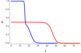
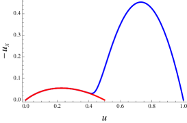
Figure 1: A numerical example of non-uniqueness of fronts (see text for details).

Example of non-uniqueness.

Clearly, uniqueness of the traveling front solutions with prescribed exponential decay cannot hold true in general, even in dimension one. Let us demonstrate such non-uniqueness by an explicit example. For simplicity, we present a numerical demonstration of existence of two traveling wave solutions with the same value of the velocity $c$, the result is then made rigorous by applying the Theorems of Sec. 2. Namely, let us consider the problem (1.3) in the one-dimensional setting with the nonlinear term $f$ given by

$$f(u)=\left\{\begin{array}[]{ll}u(1-2u),&0\leq u<\tfrac{1}{2},\\ (2u-1)(1-u)(40u-21),&\tfrac{1}{2}\leq u\leq 1.\end{array}\right.$$ (6.3)

As can be easily verified, this function satisfies conditions (H1), (H2) and (U). One may expect that for a range of velocities $c$ close to $c_{0}=2$ the problem (1.3) with nonlinearity (6.3) has two traveling front solutions: one connecting $u=0$ and $u=\tfrac{1}{2}$, and another connecting $u=0$ with $u=1$. These two solutions for $c=2.25$ are presented in Fig. 1, where Fig. 1(a) shows the traveling wave profiles and Fig. 1(b) shows the corresponding phase portraits. From the exact traveling wave solution $u(z)=\frac{3}{4}-\frac{1}{4}\tanh\left(\sqrt{5\over 2}\,z\right)$ connecting $v_{1}=\frac{1}{2}$ with $v=1$, we find that $c^{\dagger}_{v_{1}}={9\over\sqrt{10}}\approx 2.846$ (see Sec. 2 for the details of the notations). Also, by [28, Theorem 5.1] we have $c^{*}=c^{*}_{1}=2$. Therefore, since $c^{\dagger}_{v_{1}}>c^{*}$, there are two traveling wave solutions with speed $c=2.25$ by Remark 2.2, one connecting zero to $v_{1}$ and the other connecting zero to $v$. This is what we see numerically in Fig. 1. Note that the value of $c^{\sharp}$ from (2.21) is easily found to be $c^{\sharp}=\sqrt{127\over 5}\approx 5.04$.

Let us now present some heuristic arguments as to why the solutions of (1.3) and (1.2) are expected to be unique for large enough $c$. Suppose that the nonlinearity $f$ becomes strictly linear for sufficiently small $u$, i.e. we have $f(u,y)\equiv f_{u}(0,y)u$ for all $u\leq\delta$, with some $\delta>0$. In this case, clearly, the decay of any positive solution of (3.1) must be precisely

$$w(y,z)=ae^{-\lambda_{-}(c,\nu_{0})z}\,\psi_{0}(y)+\sum_{k=0}^{\infty}a_{k}^{+}e^{-\lambda_{+}(c,\nu_{k})}\,\psi_{k}(y),\qquad z\geq z_{0},$$ (6.4)

for some $z_{0}\gg 1$. Here we took into account that when $\nu_{0}<\nu_{k}\leq 0$, if ever, we have $\lambda_{-}(c,\nu_{k})<\lambda_{-}(c,\nu_{0})$, hence the presence of a term proportional to $e^{-\lambda_{-}(c,\nu_{k})z}\psi_{k}(y)$ would contradict positivity of the solution. Now, fixing the value of $a$, one can see that any two solutions of the form (6.4) differ by a function that lies in $H^{1}_{c}(\Sigma)$, since all the terms in the series in (6.4) except the first one decay exponentially with the rate strictly greater than $e^{-cz/2}$. On the other hand, it is easy to see that for $c>c^{\sharp}$, where $c^{\sharp}$ is defined in (2.21), the functional $\Psi_{c}^{w}$ is strictly convex in $H^{1}_{c}(\Sigma)$. Therefore, for every value of $a$ and every $c>c^{\sharp}$ there exists a unique positive solution of (1.3). This seems rather surprising, since, on one hand, uniqueness in this case is a consequence of convexity of $\Psi_{c}^{w}$ for $c>c^{\sharp}$, which, in some sense, is dictated by what happens in the “core” of the traveling front and thus represents a nonlinear feature of the problem. On the other hand, uniqueness also relies on the fact that, regardless of the value of $c$, any two positive solutions with the same asymptotic decay have difference that lies in $H^{1}_{c}(\Sigma)$, which is a property of the behavior far ahead of the front and represents a linear feature of the problem. From the variational point of view, uniqueness of solution is also rather surprising, since, in view of Remark 3.4, there are infinitely many auxiliary functions $w$ that can be used in the construction the functional $\Phi_{c}^{w}$ and hence, potentially, different minimizers, depending on the choice of $w$.

These heuristic arguments turn out to work in the case of generic nonlinearities in (1.3), with the result stated in Theorem 2. The proof of this theorem follows from a sequence of lemmas below.

Lemma 6.1.

We have $c^{\sharp}\geq c^{*}$.

Proof.

First, by the definition of $c^{\sharp}$ we trivially have $c^{\sharp}\geq c_{0}$. Now, take any $u\in H^{1}_{c^{\sharp}}(\Sigma)$. Then by hypothesis (H2) there exists $\tilde{u}:\Sigma\to\mathbb{R}$, with $0<\tilde{u}<u$, such that

$$\Phi_{c^{\sharp}}[u]=\int_{\Sigma}e^{c^{\sharp}z}\left(\frac{1}{2}|\nabla u|^{2}-f_{u}(\tilde{u},y)u^{2}\right)dx.$$ (6.5)

Applying the definitions of $q$ and $\hat{\nu}_{0}$ in (2.20), and the Poincaré inequality [17, Lemma 2.1], we obtain

$$\Phi_{c^{\sharp}}[u]\geq\frac{1}{2}\int_{\Sigma}e^{c^{\sharp}z}\left(u_{z}^{2}+|\nabla_{y}u|^{2}-q(y)u^{2}\right)\,dx$$

$$\geq\frac{1}{2}\int_{\Sigma}e^{c^{\sharp}z}\left({{c^{\sharp}}^{2}\over 4}+\hat{\nu}_{0}\right)u^{2}\,dx\geq 0,$$ (6.6)

implying that by (2.10) we have $c^{*}\leq c^{\sharp}$. ∎

Lemma 6.2.

Let $c>c_{0}$ and let $\bar{u}_{1}$ and $\bar{u}_{2}$ be two solutions of (1.3) and (1.2), and whose decay at $z=+\infty$ is given by (5.2). Then $\bar{u}_{2}-\bar{u}_{1}\in H^{1}_{c}(\Sigma)$.

Proof.

Introduce $h=\bar{u}_{2}-\bar{u}_{1}$, which satisfies

$$\Delta h+ch_{z}+f_{u}(0,y)h=(f_{u}(0,y)-f_{u}(\tilde{u},y))h,$$ (6.7)

for some $\tilde{u}$ bounded between $\bar{u}_{1}$ and $\bar{u}_{2}$. In view of Proposition 5.4, we have

$$0\leq\tilde{u}(y,z)\leq\min\{1,Ce^{-\lambda_{-}(c,\nu_{0})z}\},$$ (6.8)

for some $C>0$ and all $(y,z)\in\Sigma$.

Now, let $\eta\in C^{1}(\mathbb{R})$ be a cutoff function with the following properties: $\eta(z)$ is a non-increasing function of $z$ with super-exponential decay at $+\infty$, and $\eta(z)=1$ for $z\leq 0$. For fixed $\varepsilon>0$ and $c^{\prime}>0$ let us multiply (6.7) with $e^{c^{\prime}z}h\eta_{\varepsilon}^{2}$, where $\eta_{\varepsilon}(z)=\eta(\varepsilon z)$, and integrate over $\Sigma$. After a few integrations by parts, we obtain

$$\int_{\Sigma}e^{c^{\prime}z}\left(|\nabla h|^{2}-{c^{\prime}(c^{\prime}-c)\over 2}h^{2}-f_{u}(0,y)h^{2}\right)\eta_{\varepsilon}^{2}\,dx$$

$$+\int_{\Sigma}e^{c^{\prime}z}\left(2hh_{z}\eta_{\varepsilon}\eta^{\prime}_{\varepsilon}-(c^{\prime}-c)h^{2}\eta_{\varepsilon}\eta^{\prime}_{\varepsilon}\right)\,dx$$

$$=\int_{\Sigma}e^{c^{\prime}z}(f_{u}(\tilde{u},y)-f_{u}(0,y))h^{2}\eta_{\varepsilon}^{2}\,dx,$$ (6.9)

where $\eta_{\varepsilon}^{\prime}=d\eta_{\varepsilon}/dz$.

We are now going to estimate the different terms appearing in (6). Let us begin by noting that by hypothesis (H2) and (6.8) we have $|f_{u}(\tilde{u},y)-f_{u}(0,y)|\leq C|\tilde{u}(y,z)|^{\gamma}\leq C^{\prime}(1+e^{\gamma\lambda_{-}(c,\nu_{0})z})^{-1}$ for some $C,C^{\prime}>0$ and all $(y,z)\in\Sigma$. Therefore,

$$\int_{\Sigma}e^{c^{\prime}z}(f_{u}(\tilde{u},y)-f_{u}(0,y))h^{2}\eta_{\varepsilon}^{2}\,dx\leq C^{\prime}\int_{\Sigma}e^{c^{\prime}z}(1+e^{\gamma\lambda_{-}(c,\nu_{0})z})^{-1}h^{2}\eta_{\varepsilon}^{2}\,dx.$$ (6.10)

On the other hand, since $h\eta_{\varepsilon}\in H^{1}_{c^{\prime}}(\Sigma)$, by Poincaré inequality [17, Lemma 2.1] it holds

$$\int_{\Sigma}e^{c^{\prime}z}h_{z}^{2}\eta_{\varepsilon}^{2}\,dx\geq{{c^{\prime}}^{2}\over 4}\int_{\Sigma}e^{c^{\prime}z}h^{2}\eta_{\varepsilon}^{2}\,dx\hskip 85.35826pt$$

$$-2\int_{\Sigma}e^{c^{\prime}z}hh_{z}\eta_{\varepsilon}\eta^{\prime}_{\varepsilon}\,dx-\int_{\Sigma}e^{c^{\prime}z}h^{2}|\eta^{\prime}_{\varepsilon}|^{2}\,dx.$$ (6.11)

Combining this with the previous estimate and using the variational characterization of the lowest eigenvalue $\nu_{0}$ in (2.6), from (6) we obtain

$$\int_{\Sigma}e^{c^{\prime}z}\left({cc^{\prime}\over 2}-{{c^{\prime}}^{2}\over 4}+\nu_{0}\right)h^{2}\eta_{\varepsilon}^{2}\,dx\hskip 113.81102pt$$

$$-|c^{\prime}-c|\int_{\Sigma}e^{c^{\prime}z}h^{2}\eta_{\varepsilon}|\eta_{\varepsilon}^{\prime}|\,dx-\int_{\Sigma}e^{c^{\prime}z}h^{2}|\eta_{\varepsilon}^{\prime}|^{2}\,dx$$

$$\leq C\int_{\Sigma}e^{c^{\prime}z}(1+e^{\gamma\lambda_{-}(c,\nu_{0})z})^{-1}h^{2}\eta_{\varepsilon}^{2}\,dx,$$ (6.12)

for some $C>0$ independent of $\varepsilon$.

To proceed, we need to choose the cutoff function $\eta$ in such a way that the terms involving $\eta_{\varepsilon}^{\prime}$ can be bounded by the terms involving $\eta_{\varepsilon}$ uniformly in $\varepsilon$ as $\varepsilon\to 0$. This can be achieved by setting $\eta(z)=\exp(-\tfrac{1}{2}z^{2})$ for $z>0$. Indeed, consider the last term in the left-hand side of (6). We can write

$$\int_{\Sigma}e^{c^{\prime}z}h^{2}|\eta_{\varepsilon}^{\prime}|^{2}\,dx\leq\alpha^{2}\int_{\Sigma}e^{c^{\prime}z}h^{2}\eta_{\varepsilon}^{2}\,dx+\int_{\{|\eta^{\prime}_{\varepsilon}|\geq\alpha\eta\}}e^{c^{\prime}z}h^{2}|\eta_{\varepsilon}^{\prime}|^{2}\,dx,$$ (6.13)

for any $\alpha>0$. From our choice of $\eta$, the second integral is over all $z\geq\alpha\varepsilon^{-2}$. Therefore, assuming $h\in L^{2}_{c^{\prime\prime}}(\Sigma)$ for some $c^{\prime\prime}\in(0,c^{\prime})$, we have

$$\int_{\Sigma}e^{c^{\prime}z}h^{2}|\eta_{\varepsilon}^{\prime}|^{2}\,dx\leq\alpha^{2}\int_{\Sigma}e^{c^{\prime}z}h^{2}\eta_{\varepsilon}^{2}\,dx+\int_{\alpha\varepsilon^{-2}}^{\infty}\int_{\Omega}e^{c^{\prime}z}h^{2}|\eta_{\varepsilon}^{\prime}|^{2}\,dydz$$

$$\leq\alpha^{2}\int_{\Sigma}e^{c^{\prime}z}h^{2}\eta_{\varepsilon}^{2}\,dx+C_{\varepsilon}\int_{\Sigma}e^{c^{\prime\prime}z}h^{2}\,dx,$$ (6.14)

where

$$C_{\varepsilon}=\sup_{z\geq\alpha\varepsilon^{-2}}\left(e^{(c^{\prime}-c^{\prime\prime})z}|\eta_{\varepsilon}^{\prime}(z)|^{2}\right).$$ (6.15)

Similarly,

$$\int_{\Sigma}e^{c^{\prime}z}h^{2}\eta_{\varepsilon}|\eta_{\varepsilon}^{\prime}|\,dx\leq\alpha\int_{\Sigma}e^{c^{\prime}z}h^{2}\eta_{\varepsilon}^{2}\,dx+\alpha^{-1}C_{\varepsilon}\int_{\Sigma}e^{c^{\prime\prime}z}h^{2}\,dx.$$ (6.16)

Therefore, we can rewrite (6) in the following form (also taking (2.9) into consideration)

$$\int_{\Sigma}e^{c^{\prime}z}\left({cc^{\prime}\over 2}-{{c^{\prime}}^{2}\over 4}-{c_{0}^{2}\over 4}-\alpha|c^{\prime}-c|-\alpha^{2}\right)h^{2}\eta_{\varepsilon}^{2}\,dx$$

$$\leq C\sup_{z\in\mathbb{R}}\left({e^{(c^{\prime}-c^{\prime\prime})z}\over 1+e^{\gamma\lambda_{-}(c,\nu_{0})z}}\right)\int_{\Sigma}e^{c^{\prime\prime}z}h^{2}\,dx$$

$$+C_{\varepsilon}\left(1+{|c^{\prime}-c|\over\alpha}\right)\int_{\Sigma}e^{c^{\prime\prime}z}h^{2}\,dx,$$ (6.17)

for some $C>0$ independent of $\varepsilon$.

Now, by an explicit computation, we have

$$C_{\varepsilon}=\sup_{\zeta\geq 1}\left(\alpha^{2}\zeta^{2}\exp(-\varepsilon^{-2}(\alpha^{2}\zeta^{2}-(c^{\prime}-c^{\prime\prime})\alpha\zeta))\right)\leq\alpha^{2},$$ (6.18)

as soon as $c^{\prime}-c^{\prime\prime}<\alpha$ and $\varepsilon$ is small enough. Introducing the constants

$$c_{\pm}=c\pm\sqrt{c^{2}-c_{0}^{2}},$$ (6.19)

and using (6.18), we then find that (6) is equivalent to

$$\Bigl{\{}(c^{\prime}-c_{-})(c_{+}-c^{\prime})-8\alpha|c-c^{\prime}|\Bigr{\}}\int_{\Sigma}e^{c^{\prime}z}h^{2}\eta_{\varepsilon}^{2}\,dx\leq C\int_{\Sigma}e^{c^{\prime\prime}z}h^{2}\,dx,$$ (6.20)

with $C>0$ independent of $\varepsilon$, whenever $c^{\prime}-c^{\prime\prime}<\alpha\leq\min(\gamma\lambda_{-}(c,\nu_{0}),|c^{\prime}-c|)$ and $\varepsilon$ is sufficiently small.

We now note that by Proposition 5.4 we have $h\in L^{2}_{c^{\prime\prime}}(\Sigma)$ for some $c^{\prime\prime}\in(c_{-},c_{+})$. Therefore, we can choose $c^{\prime}=c^{\prime\prime}+\tfrac{1}{2}\alpha$, with $\alpha$ so small that the quantity in the curly brackets in (6.20) is positive. Then, passing to the limit $\varepsilon\to 0$ in (6.20), by monotone convergence theorem we can conclude that, in fact, we have $h\in L^{2}_{c^{\prime}}(\Sigma)$. Applying the same argument to (6) we find that also $h\in H^{1}_{c^{\prime}}(\Sigma)$, with $c^{\prime}\in(c^{\prime\prime},c_{+})$. Finally, iterating this argument, we find that

$$h\in H^{1}_{c^{\prime}}(\Sigma),\qquad\forall c^{\prime}<c_{+}.$$ (6.21)

In particular, $h\in H^{1}_{c}(\Sigma)$, which completes the proof. ∎

Lemma 6.3.

Let $c>c^{\sharp}$. Then the functional $\Psi_{c}^{w}$ is strictly convex on $\mathcal{A}_{c}^{w}$.

Proof.

First of all, let us point out that due to the presence of the exponential weight the functional $\Psi_{c}^{w}$ is not twice continuously differentiable in $H^{1}_{c}(\Sigma)$, so the convexity of the functional cannot be concluded by evaluating the second variation of $\Psi_{c}^{w}$. Nevertheless, what we will show below is that the functional $\Psi_{c}^{w}$ is strongly convex [29], i.e., there exists $\sigma>0$ such that for every $h_{1},h_{2}\in\mathcal{A}_{c}^{w}$ it holds

$$\Psi_{c}^{w}[h_{2}]\geq\Psi_{c}^{w}[h_{1}]+\delta\Psi_{c}^{w}(h_{1},h_{2}-h_{1})+{\sigma\over 2}||h_{2}-h_{1}||^{2}_{L^{2}_{c}(\Sigma)}.$$ (6.22)

Indeed, by hypothesis (H2) we have

$$\Psi_{c}^{w}[h_{2}] = \Psi_{c}^{w}[h_{1}]+\delta\Psi_{c}^{w}(h_{1},h_{2}-h_{1})+\frac{1}{2}\int_{\Sigma}e^{cz}|\partial_{z}(h_{2}-h_{1})|^{2}dx$$ (6.23)

$$+ \frac{1}{2}\int_{\Sigma}e^{cz}\left(|\nabla_{y}(h_{2}-h_{1})|^{2}-f_{u}(\tilde{u},y)(h_{2}-h_{1})^{2}\right)dx,$$

for some $0\leq\tilde{u}\leq 1$. Now, by Poincaré inequality [17, Lemma 2.1], we have

$$\frac{1}{2}\int_{\Sigma}e^{cz}|\partial_{z}(h_{2}-h_{1})|^{2}dx\geq{c^{2}\over 8}||h_{2}-h_{1}||^{2}_{L^{2}_{c}(\Sigma)},$$ (6.24)

and by the definition of $\hat{\nu}_{0}$ in (2.20)

$$\frac{1}{2}\int_{\Sigma}e^{cz}\left(|\nabla_{y}(h_{2}-h_{1})|^{2}-f_{u}(\tilde{u},y)(h_{2}-h_{1})^{2}\right)dx\geq{\hat{\nu}_{0}\over 2}||h_{2}-h_{1}||^{2}_{L^{2}_{c}(\Sigma)}.$$ (6.25)

Strong convexity then follows with $\sigma=\tfrac{1}{4}c^{2}+\hat{\nu}_{0}>0$, in view of $c>c^{\sharp}$ and implies strict convexity [29, Chapter 12.H^∗]. ∎

Proof of Theorem 3.

Let $\bar{u}_{1}$ and $\bar{u}_{2}$ be as in Lemma 6.2. Without loss of generality we may assume that $a$ is sufficiently small in (5.2). Let us define $w$ to be a suitably truncated version of $\bar{u}_{1}$. Then, by hypothesis (H2) the functional $\Psi_{c}^{w}$ is of class $C^{1}$ and by Lemma 6.3 is also strictly convex on $\mathcal{A}_{c}^{w}$. Then $h_{1}:=\bar{u}_{1}-w$ belongs to $\mathcal{A}_{c}^{w}$. In fact, the function $h_{2}:=\bar{u}_{2}-w$ also belongs to $\mathcal{A}_{c}^{w}$, in view of Lemma 6.2. On the other hand, since the equivalent functional $\Phi_{c}^{w}$ is also strictly convex, it has at most one critical point. Therefore, since $\bar{u}_{1}$ and $\bar{u}_{2}$ solve the Euler-Lagrange equation (1.3) for $\Phi_{c}^{w}$ and are, therefore, critical points of $\Phi_{c}^{w}$, we conclude that $\bar{u}_{1}=\bar{u}_{2}$. ∎

7 Global asymptotic stability of fast fronts

We now investigate the stability properties of traveling wave solutions with speed $c>c^{*}$ obtained in the preceding sections. Let us point out in the first place that one cannot expect these traveling wave solutions to be stable in the usual sense (say, with respect to small $L^{\infty}$ perturbations). Indeed, under hypotheses (H1), (H2) and (U) a truncation of the traveling wave solution with any $c>c^{*}$ by a cutoff function that vanishes identically for all $z\geq R\gg 1$ would not converge to the corresponding traveling wave, but will instead propagate with the asymptotic speed $c^{*}$ of the critical front [18, Theorem 5.8]. Similarly, modifying the rate of exponential decay in front of the traveling wave solution with speed $c>c^{*}$ may lead to acceleration or slowdown of the front (see e.g. [30, 31, 32]), or even lead to irregular behavior [33]. Therefore, stability of these traveling wave solutions should be considered with respect to suitable classes of perturbations [30, 34]. Here we show global stability of the (unique) supercritical traveling waves with $c>c^{\sharp}$ under perturbations lying in the weighted space $L^{2}_{c^{\prime}}(\Sigma)$ with suitably chosen $c^{\prime}>0$.

We begin with a general existence result for the solutions of (1.1) of the form

$$u(y,z,t)=\bar{u}(y,z-ct)+w(y,z-ct,t),$$ (7.1)

where $\bar{u}$ is given by Theorem 1 with some fixed $c>c^{*}$, and $w$ lying in an appropriate exponentially weighted space. The function $w$ satisfies the following parabolic equation

$$w_{t}=\Delta w+cw_{z}+f(\bar{u}+w,y)-f(\bar{u},y).$$ (7.2)

Easily adapting [20, Proposition 3.1] (see also [18]), we can obtain the following basic existence and regularity result for the initial value problem associated with (7.2):

Proposition 7.1.

For any $c^{\prime}>0$, let $w_{0}\in L^{2}_{c^{\prime}}(\Sigma)$ and let $0\leq\bar{u}+w\leq 1$. Then there exists a unique solution $w\in C^{\alpha}((0,\infty);H^{2}_{c^{\prime}}(\Sigma))\cap C^{1,\alpha}((0,+\infty);L^{2}_{c^{\prime}}(\Sigma))\cap C([0,+\infty);L^{2}_{c^{\prime}}(\Sigma))$, for all $\alpha\in(0,1)$, of (7.2) and the same boundary conditions as in (1.2), such that $w(x,0)=w_{0}(x)$.

We are now in a position to complete the proof of Theorem 3, following the method introduced in [16].

Proof of Theorem 3.

Without loss of generality, we may assume that $c^{\prime}<2\lambda_{+}(c,\hat{\nu}_{0})$, where $\lambda_{\pm}(c,\nu)$ are defined in (2.11). The result in Proposition 7.1 implies that we can multiply (7.2) by $e^{c^{\prime}z}w$ and integrate over $\Sigma$. Using hypothesis (H2) and the definition of $q(y)$ in (2.20), we have

$$\int_{\Sigma}e^{c^{\prime}z}ww_{t}\,dx\leq\int_{\Sigma}e^{c^{\prime}z}\left(\Delta w+cw_{z}-q(y)w\right)w\,dx.$$ (7.3)

Then, after a number of integrations by parts, we obtain

$${d\over dt}\int_{\Sigma}e^{c^{\prime}z}w^{2}\,dx\leq-2\int_{\Sigma}e^{c^{\prime}z}\left(w_{z}^{2}+{c^{\prime}(c-c^{\prime})\over 2}w^{2}+|\nabla_{y}w|^{2}-q(y)w^{2}\right)dx.$$ (7.4)

Applying the Poincaré inequality [17, Lemma 2.1] and the definition of $\hat{\nu}_{0}$ in (2.20), we then arrive at

$${d\over dt}\int_{\Sigma}e^{c^{\prime}z}w^{2}dx\leq 2\left({{c^{\prime}}^{2}\over 4}-{cc^{\prime}\over 2}-\hat{\nu}_{0}\right)\int_{\Sigma}e^{c^{\prime}z}w^{2}\,dx$$

$$=\frac{1}{2}\{c^{\prime}-2\lambda_{-}(c,\hat{\nu}_{0})\}\{c^{\prime}-2\lambda_{+}(c,\hat{\nu}_{0})\}\int_{\Sigma}e^{c^{\prime}z}w^{2}\,dx.$$ (7.5)

Therefore, since $c^{\prime}\in(2\lambda_{-}(c,\hat{\nu}_{0}),2\lambda_{+}(c,\hat{\nu}_{0}))$, the coefficient in front of the integral in the right-hand side of (7) is negative, which implies exponential decay of the $L^{2}_{c^{\prime}}$-norm of $w$. ∎

References

- [1] J. D. Murray. Mathematical Biology. Springer-Verlag, Berlin, 1989.
- [2] R. Kapral and K. Showalter, editors. Chemical waves and patterns. Kluwer, Dordrecht, 1995.
- [3] Ya. B. Zeldovich, G. I. Barenblatt, V. B. Librovich, and G. M. Makhviladze. The Mathematical Theory of Combustion and Explosions. Consultants Bureau, New York, 1985.
- [4] J. Keener and J. Sneyd. Mathematical Physiology. Springer-Verlag, New York, 1998.
- [5] P. C. Fife. Mathematical Aspects of Reacting and Diffusing Systems. Springer-Verlag, Berlin, 1979.
- [6] A. G. Merzhanov and E. N. Rumanov. Physics of reaction waves. Rev. Mod. Phys., 71:1173–1210, 1999.
- [7] W. van Saarloos. Front propagation into unstable states. Phys. Rep., 386:29–222, 2003.
- [8] C. B. Muratov and M. Novaga. Front propagation in infinite cylinders. II. The sharp reaction zone limit. Calc. Var. PDE, 31:521–547, 2008.
- [9] H. Berestycki and F. Hamel. Front propagation in periodic excitable media. Comm. Pure Appl. Math., 55:949–1032, 2002.
- [10] A. N. Kolmogorov, I. G. Petrovsky, and N. S. Piskunov. Study of the diffusion equation with growth of the quantity of matter and its application to a biological problem. Bull. Univ. Moscow, Ser. Int., Sec. A, 1:1–25, 1937.
- [11] H. Berestycki and L. Nirenberg. Traveling fronts in cylinders. Ann. Inst. H. Poincaré Anal. Non Linéaire, 9:497–572, 1992.
- [12] J. M. Vega. Travelling wavefronts of reaction-diffusion equations in cylindrical domains. Comm. Partial Differential Equations, 18:505–531, 1993.
- [13] J. M. Vega. The asymptotic behavior of the solutions of some semilinear elliptic equations in cylindrical domains. J. Differ. Equations, 102:119–152, 1993.
- [14] S. Heinze. Travelling waves for semilinear parabolic partial differential equations in cylindrical domains. SFB 123 Preprint 506, University of Heidelberg, 1989.
- [15] S. Heinze. A variational approach to traveling waves. Technical Report 85, Max Planck Institute for Mathematical Sciences, Leipzig, 2001.
- [16] C. B. Muratov. A global variational structure and propagation of disturbances in reaction-diffusion systems of gradient type. Discrete Cont. Dyn. S., Ser. B, 4:867–892, 2004.
- [17] M. Lucia, C. B. Muratov, and M. Novaga. Existence of traveling waves of invasion for Ginzburg-Landau-type problems in infinite cylinders. Arch. Rational Mech. Anal., 188:475–508, 2008.
- [18] C. B. Muratov and M. Novaga. Front propagation in infinite cylinders. I. A variational approach. Comm. Math. Sci., 6:799–826, 2008.
- [19] J. M. Vega. On the uniqueness of multidimensional travelling fronts of some semilinear equations. J. Math. Anal. Appl., 177:481–490, 1993.
- [20] C. B. Muratov and M. Novaga. Global stability and exponential convergence to variational traveling waves in cylinders. SIAM J. Math. Anal., submitted.
- [21] R. A. Fisher. The advance of advantageous genes. Ann. Eugenics, 7:355–369, 1937.
- [22] L. C. Evans and R. L. Gariepy. Measure Theory and Fine Properties of Functions. CRC, Boca Raton, 1992.
- [23] D. Gilbarg and N. S. Trudinger. Elliptic Partial Differential Equations of Second Order. Springer-Verlag, Berlin, 1983.
- [24] D. Kinderlehrer and G. Stampacchia. An Introduction to Variational Inequalities and Their Applications. Academic Press, New York, 1980.
- [25] B. Kawohl. Rearrangements and Convexity of Level Sets in PDE. Springer-Verlag, Berlin, 1985.
- [26] M. Bertsch and I. Primi. Traveling wave solutions of the heat flow of director fields. Ann. Inst. H. Poincaré Anal. Non Linéaire, 24:227–250, 2007.
- [27] H. Berestycki and L. Nirenberg. On the method of moving planes and the sliding method. Bol. Soc. Brasil. Mat. (N.S.), 22(1):1–37, 1991.
- [28] M. Lucia, C. B. Muratov, and M. Novaga. Linear vs. nonlinear selection for the propagation speed of the solutions of scalar reaction-diffusion equations invading an unstable equilibrium. Commun. Pure Appl. Math., 57:616–636, 2004.
- [29] R. T. Rockafellar and R. J.-B. Wets. Variational analysis, volume 317 of Grundlehren der Mathematischen Wissenschaften [Fundamental Principles of Mathematical Sciences]. Springer-Verlag, Berlin, 1998.
- [30] D. H. Sattinger. On the stability of waves of nonlinear parabolic systems. Advances in Math., 22:312–355, 1976.
- [31] M. Bramson. Convergence to traveling waves for systems of Kolmogorov-like parabolic equations. In Nonlinear diffusion equations and their equilibrium states, I (Berkeley, CA, 1986), volume 12 of Math. Sci. Res. Inst. Publ., pages 179–190. Springer, New York, 1988.
- [32] J.-F. Mallordy and J.-M. Roquejoffre. A parabolic equation of the KPP type in higher dimensions. SIAM J. Math. Anal., 26:1–20, 1995.
- [33] E. Yanagida. Irregular behavior of solutions for Fisher’s equation. J. Dynam. Differential Equations, 19:895–914, 2007.
- [34] D. Sattinger. Weighted norms for the stability of the traveling waves. J. Differential Equations, 25:130–144, 1977.