Quantum energy teleportation in a quantum Hall system

Abstract

We propose an experimental method for a quantum protocol termed quantum energy teleportation (QET), which allows energy transportation to a remote location without physical carriers. Using a quantum Hall system as a realistic model, we discuss the physical significance of QET and estimate the order of energy gain using reasonable experimental parameters.

I Introduction

The phenomenon of quantum teleportation (QT) has been experimentally demonstrated in quantum optics QT ; exp-QT . But as is well known, this protocol can teleport only information (i.e., quantum mechanical information or quantum states) and not physical objects. Thus, this protocol cannot teleport energy because that requires a physical entity to act as an energy carrier. For example, electricity is transported over power transmission lines by electromagnetic waves that act as the carrier. Recently, however, one of the authors proposed a quantum protocol termed quantum energy teleportation (QET) that avoids the problem by using classical information instead of energy carriers hotta . In this counterintuitive protocol, the counterpart of the classical “transmission line”is a quantum mechanical many-body system in the vacuum state (i.e., a correlated system formed by vacuum state entanglement R .) The key lies using this correlated system (hereinafter, the quantum correlation channel) to exploit the zero-point energy of the vacuum state, which stems from zero-point fluctuations (i.e., nonvanishing vacuum fluctuations) originating from the uncertainty principle. This energy, however, cannot be conventionally extracted casimir as that would require a state with lower energy than vacuum—a contradiction. In fact, no local operation can extract energy from vacuum, but must instead inject energy; this property is called passivity passivity . According to QET, however, if we limit only the local vacuum state instead of all the vacuum states, the passivity of the local vacuum state can be destroyed and a part of the zero-point energy can in fact be extracted.

As schematically illustrated in Fig. 1, a QET system to transfer energy from subsystem A to B consists of four elements: (i) a quantum correlation channel, (ii) a local measurement system for subsystem A defined on the quantum correlation channel, (iii) a classical channel for communicating the measurement result, and (iv) a local operation system for subsystem B. Essentially, QET can be regarded as quantum feedback protocol implemented via local operations and classical communication (LOCC). The procedure is as follows: First, we measure the local field fluctuations at subsystem A. The obtained result includes information about local fluctuations at subsystem B because of the vacuum state entanglement via the quantum correlation channel R . This is because the kinetic energy term in the field Hamiltonian generates the entanglement and provides partial correlation between local vacuum fluctuations. Thus, owing to passivity of the vacuum state, the measurement causes some energy ($E_{A}$) to be injected into subsystem A. Next, the obtained result is communicated to subsystem B via a classical channel. Since the measurement performed at subsystem A is local, subsystem B remains in a local vacuum state. As mentioned above, if a good local operation is performed at subsystem B using the information gained at subsystem A, it will be possible to extract some amount of the zero-point energy of subsystem B, $E_{B}$. Thus, this protocol only gives “permission” to use the otherwise unavailable energy at B. If we define ”teleportation” as a process of transferring energy to a remote location without a physical energy carrier, we can say that energy is teleported by this protocol.

Although the validity of this protocol has been confirmed mathematically, its physical significance remains questionable: What type of physical system is necessary for implementing QET? What is the composition of the quantum correlation channel? Can significant amounts of energy be “teleported”? Unfortunately, all past proposals for experimental verification of QET cannot teleport sufficient amounts of energy to be measured with present technology cold ions ; EM field . Here, we discuss a more realistic possible implementation and estimate the order of the “teleported” energy using reasonable experimental parameters.

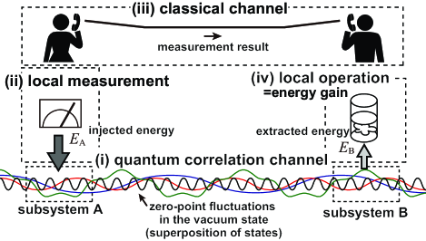
Figure 1: (color online). Schematic diagram of the quantum energy teleportation (QET) protocol.

II Overview of QET protocol in the quantum Hall system

Verification of QET in a realistic system requires the following: (i) a dissipationless system, (ii) a quantum correlation channel with a macroscopic correlation length, (iii) detection and operation schemes for well-defined fluctuations in the vacuum state, and (iv) a suitable implementation of LOCC.

To this end, we consider a quantum Hall (QH) system as a potential candidate. The QH effect is observed in two-dimensional (2D) electron systems in semiconductors subjected to a strong perpendicular magnetic field Yoshioka . The QH system satisfies requirement (i) because the QH effect does not offer any resistance. Further, in this system, quasi-one-dimensional channels called edge channels appear at the boundary of the 2D incompressible region of the QH system (i.e., QH bulk). Such an edge channel can behave as a chiral Luttinger liquid wen , along which electric current flows in a unidirectional manner. This attribute is indicative of the chirality of the edge channel. Moreover, in experiments, the edge channel shows power-law behaviors and does not have a specific decay length chang ; grayson , preferable for fairly long-distance teleportation. Thus, an edge channel satisfies requirement (ii). Furthermore, an edge channel can be universally characterized by charge fluctuations described by a gapless free boson field in the vacuum state, independently of the detailed structures of the QH bulk state. Therefore, the target zero-point fluctuation is the fluctuation of the charge density wave (i.e., a magnetoplasmon allen ) propagating in a unidirectional manner along an edge channel). This implies that owing to the Coulomb interaction, a conventional capacitor can be used as a sensitive probe and control method for detecting and manipulating zero-point fluctuations of vacuum. Given these facts, it can be said that (iii) is satisfied. Lastly, for a QH system, semiconductor nanotechnology can be used to design on-chip LOCC, thus satisfying requirement (iv).

As shown in Fig. 2, element (i), i.e., the quantum correlation channel, is the left-going edge channel $S$. To produce the vacuum state, $S$ should be connected to an ideal electric ground, and experiments should be performed at low temperatures—on the order of millikelvin (mK). Regions A and B, physically corresponding to subsystems A and B, respectively, are defined by fabricating micrometer-scale metal gate electrodes (i.e., a microscopic capacitor) on $S$.

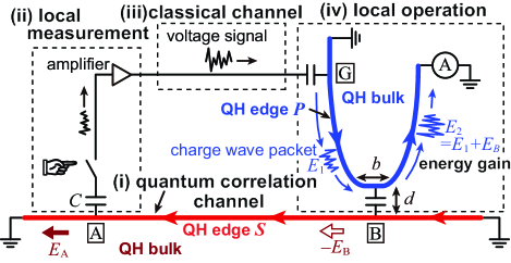
Figure 2: (color online). Schematic diagram of the QH system used in this study. Edge channels $S$ and $U$ are formed at the boundaries of QH bulk regions $S$ and $U$, respectively. The red and blue arrows indicate the directions of propagation of charge waves.

Element (ii), used for local measurement of the zero-point fluctuations (i.e., charge fluctuations), comprises a metal gate electrode fabricated on $S$ at region A as well as an amplifier and a switch. The input resistance $R$ of the amplifier and capacitance $C$ between $S$ and the gate electrode at region A constitute an RC circuit. When the switch is turned on, the information on the charge fluctuations in $S$ is imprinted on the quantum voltage fluctuations of the electric circuit via the Coulomb interaction and then enhanced by the amplifier. Here, the on-chip electrical circuit serves the function of the voltmeter shown in the schematic in Fig. 1. As explained later, we can assume that this RC circuit and amplifier can operate fast enough, and the circuit can be considered as performing a positive operator valued measure (POVM)-type measurement chang . The amplified signal $\upsilon$ (i.e., measurement result) is transferred through a classical channel (element (iii)), which corresponds to an electric wire.

Element (iv), used for the local operation, includes another edge channel $P$ placed such that $P$ and $S$ approach each other at region B. It also consists of a metal gate electrode fabricated on $P$ at region G and a measurement instrument such as a picoammeter (Fig. 2).

The experimental procedure is a follows: First, we cool down the entire system, except the measurement instruments, to the lowest temperature possible (on the order of several mK) to achieve the vacuum state. Next, we turn on the switch only for a period of $\tau_{m}$. When a voltage signal $\upsilon$ arrives at region G, it excites a charge wave packet on $P$ via capacitive coupling. Because of the chirality of the edge channel, the charge wave packet travels in a unidirectional manner along $P$, carrying energy $E_{1}$ toward region B, where the wave packet interacts with the zero-point fluctuation of $S$chirarity . Then, the energy carried by the wave packet changes from $E_{1}$ to $E_{2}$. Finally, we measure the signal with the picoammeter connected to $P$ and thereby estimate the energy carried by the wave packet. This is a unit cycle of a single-shot measurement. We may repeat this single-shot measurement a sufficient number of times to generate meaningful statistics. Finally, we can use the results to estimate the average energy $\langle E_{2}\rangle$ carried by the wave packets. To verify that QET is actually occurring, we must also perform a control experiment in which region G is disconnected from the classical channel and instead connected to a signal generator to excite wave packets independently of $\upsilon$. If wave packets are created by the signal generator (i.e., no information about $\upsilon$ is communicated), they will inject energy into $S$ because of the passivity of the vacuum state passivity . Thus, $E_{B}=E_{2}-E_{1}$ will be negative. However, in our system, since wave packets explicitly depend on $\upsilon$, passivity is disturbed and $\langle E_{2}\rangle$ can take a positive value; in other words, positive energy is extracted from the zero-point fluctuations of $S$. Finally, if $\langle E_{2}\rangle$ is larger in QET experiment than in the control, we can conclude the QET theory is valid—energy is “teleported” from A to B without physical carriers to transport that energy. In what follows, we prove this argument theoretically and estimate $E_{B}$ by setting the experimental parameters $R\sim 10~{}$k$\Omega$ impedance ; $C\sim 10$ fF; and $v_{g}\sim 10^{6}$ m/s ashoori ; kamata , were $v_{g}$ is the group velocity of a charge density wave. Length $b$ of regions G and B and the length of region A are approximated by a typical length scale of $l\sim 10~{}\mu$m.

III QET formulation in the QH system

III.1 Formulation of chiral edge channel and local measurement of charge fluctuations

Here we discuss the chiral field of the edge channels. Details on the treatment of the chiral field can be found in the literature Yoshioka .  Let us start the detailed discussion with a model of the edge channel $S$. The chiral field operator $\varrho_{S}(x)$ satisfies a commutation relation, $\left[\varrho_{S}(x),~{}\varrho_{S}(x^{\prime})\right]=i\frac{\nu}{2\pi}\partial_{x}\delta(x-x^{\prime})$. The energy density operator of $\varrho_{S}(x)$ is written as

$$\varepsilon_{S}(x)=\frac{\pi\hbar v_{g}}{\nu_{S}}:\varrho_{S}\left(x\right)^{2}:,$$

where $\nu_{S}$ is the Landau level filling factor of $S$ and $::$ denotes normal ordering, which makes the expectation value of $\varepsilon_{S}(x)$ to be zero for the vacuum state $|0_{S}\rangle$; $\langle 0_{S}|\varepsilon_{S}(x)|0_{S}\rangle=0$. The free Hamiltonian of $S$ is given by $H_{S}=\int_{-\infty}^{\infty}\varepsilon_{S}(x)dx$. The eigenvalue of the vacuum state vanishes: $H_{S}|0_{S}\rangle=0$. If the vacuum state is not entangled, the two-point correlation function of $\langle 0_{S}|\varrho_{S}(x_{A})\varrho_{S}(x_{B})|0_{S}\rangle$ with $x_{A}\neq x_{B}$ is exactly zero. However, this entangled vacuum state provides a nontrivial correlation:

$$\langle 0_{S}|\varrho_{S}(x_{A})\varrho_{S}(x_{B})|0_{S}\rangle=-\frac{\nu_{S}}{4\pi^{2}\left(x_{A}-x_{B}\right)^{2}}.$$

This correlation function can be calculated by using creation and annihilation operators of the free field. Taking region A for $x\in\left[a_{-},~{}a_{+}\right]$, we adopt the RC-circuit-detector model proposed by Fève et al. Feve to measure the voltage induced by the zero-point fluctuations of $\varrho_{S}(x)$. The charge fluctuation at A is estimated as

$$Q_{S}(t)=e\int_{-\infty}^{\infty}\varrho_{S}\left(x+v_{g}t\right)w_{A}(x)dx$$ (1)

with a window function $w_{A}(x)$ that equals 1 in $x\in\left[a_{-},~{}a_{+}\right]$ and decays rapidly outside A. In this model Feve , the voltage at the contact point between the detector and $S$ is given by $V(t)=\frac{1}{C}\left[Q_{S}(t)-Q(t)\right]$, where $Q(t)$ is the charge of the capacitor. The coupled Hamiltonian of $S$ and the RC circuit can be directly diagonalized, enabling analytical estimation of various physical quantities Feve . For example, the quantum noise of the voltage $V(t)$ is described by an operator $\hat{V}$ defined by

$$\hat{V} =-\sqrt{\frac{\hbar}{\pi RC^{2}}}$$

$$\times\int_{0}^{\infty}d\omega\left[\frac{\sqrt{\omega}}{\omega-\frac{1}{iRC}}a_{in}(\omega)+\frac{\sqrt{\omega}}{\omega+\frac{1}{iRC}}a_{in}^{{\dagger}}(\omega)\right],$$ (2)

where $a_{in}(\omega)$($a_{in}(\omega)^{{\dagger}}$) is the annihilation (creation) operator of excitation of the charge density wave in the local-measurement RC circuit and $\left[a_{in}(\omega),~{}a_{in}(\omega^{\prime})^{{\dagger}}\right]=\delta\left(\omega-\omega^{\prime}\right)$. Prior to the measurement (i.e., the signal input from $S$ to the detector), $V(t=-0)$ equals $\hat{V}$. Using the fast detector condition ($RC\ll l/v_{g}$), the voltage after the measurement is computed as

$$V(t=+0)=\hat{V}+R\dot{Q}_{S}(0),$$ (3)

where $R\dot{Q}_{S}(0)$ denotes the voltage shift induced by the signal and the dot in $\dot{Q}_{S}(0)$ stands for the time derivative. Using Eq. (2), the amplitude $\Delta V$ of $\hat{V}$ in the vacuum state $|0_{RC}\rangle$ of the RC circuit can be estimated as

$$\Delta V=\sqrt{\langle 0_{RC}|\hat{V}^{2}|0_{RC}\rangle}\sim\sqrt{\frac{\hbar}{RC^{2}}},$$

which is expected to be on the order of $10$ $\mu$V. From Eq.(1), the root-mean-square value of the voltage sift,$\sqrt{\langle 0_{S}|\left(R\dot{Q}_{S}(0)\right)^{2}|0_{S}\rangle}$, is estimated to be on the order of $100~{}\mu$V, showing that the quantum fluctuations of the edge current are detectable.

Now, we estimate the corresponding measurement operators nc of this voltage measurement. Clearly, this is difficult to achieve with sufficient accuracy with a microscopic model. However, after the amplification of the quantum noise of the voltage $V(t)$, the signal becomes macroscopic and classical. Thus, we may estimate the measurement operators of the macroscopic system comprising subsystem A, the amplifier, and the electric wire by reducing the measurement to the pointer-basis proposed by von Neumann vN . For this, let us begin with a gedankenexperiment in which a high-speed voltage meter is connected to the amplifier. Thus, the position of the meter pointer instantaneously shifts according to the signal strength. Assume that the pointer shift is equal to Eq. (3). In the same manner as that used by von Neumann vN , we can treat the macroscopic system including this voltage meter with quantum mechanics, even though the meter is macroscopic and classical. The readout of the meter pointer can be, therefore, treated as a kind of quantum measurement, which can be described by measurement operators $M_{v}$ nc with the output value of $v$. The shift of the meter pointer, $R\dot{Q}_{S}(0)$, in Eq. (3) can be reproduced by a macroscopic measurement Hamiltonian given by

$$H_{m}(t)=\hbar\delta(t)R\dot{Q}_{S}(0)P_{\hat{V}},$$

where $P_{\hat{V}}$ is the conjugate momentum operator of $\hat{V}$. In fact, the time evolution generated by this effective Hamiltonian is given by

$$U_{m}=\operatorname*{T}\exp\left(-\frac{i}{\hbar}\int_{-0}^{+0}H_{m}(t)dt\right)=\exp\left(-iR\dot{Q}_{S}(0)P_{\hat{V}}\right)$$

with time-ordered exponentiation, $\operatorname*{T}\exp$, of the time dependent Hamiltonian and reproduces Eq. (3) as follows:

$$U_{m}^{{\dagger}}\hat{V}U_{m}=V(t=+0)=\hat{V}+R\dot{Q}_{S}(0).$$

We are able to derive the measurement operators $M_{v}$ by using $U_{m}$. Firstly, using the eigenvalue $\upsilon$ of $\hat{V}$ ($\hat{V}|\upsilon\rangle=\upsilon|\upsilon\rangle$), we can assume the initial wavefunction of the quantum pointer in the $\upsilon$ representation as

$$\Psi_{i}(\upsilon)\varpropto\exp\left[-\frac{1}{4\Delta V^{2}}\upsilon^{2}\right],$$

whereas the wavefunction after the measurement is translated as

$$\Psi_{f}(\upsilon)\varpropto\exp\left[-\frac{1}{4\Delta V^{2}}\left(\upsilon-R\dot{Q}_{S}(0)\right)^{2}\right],$$

using $U_{m}$. Next, after turning the measurement interaction on (i.e., turning the switch on), we perform a projective measurement of $\hat{V}$ to obtain an eigenvalue $\upsilon$ of $\hat{V}$. This reduction analysis proves the measurement operator $M_{\upsilon}$ being $\Psi_{f}(\upsilon)$:

$$M_{\upsilon}=\left(\frac{1}{2\pi\Delta V^{2}}\right)^{1/4}\exp\left[-\frac{1}{4\Delta V^{2}}\left(\upsilon-R\dot{Q}_{S}(0)\right)^{2}\right].$$

The corresponding POVM is given by $\Pi_{\upsilon}=M_{\upsilon}^{{\dagger}}M_{\upsilon}$ and satisfies the standard sum rule: $\int_{-\infty}^{\infty}\Pi_{\upsilon}d\upsilon=I_{S}$, where $I_{S}$ is the identity operator of the Hilbert space of $\varrho_{S}(x)$. The emergence probability density of the result being $\upsilon$ is $p(\upsilon)=\langle 0_{S}|\Pi_{\upsilon}|0_{S}\rangle$. The post-measurement state of $\varrho_{S}\left(x\right)$ corresponding to the result $\upsilon$ is computed as $M_{\upsilon}|0_{S}\rangle$ up to the normalization constant. Hence, the average state of $\varrho_{S}\left(x\right)$ right after the measurement is given by

$$\rho_{1}=\int_{-\infty}^{\infty}M_{\upsilon}|0_{S}\rangle\langle 0_{S}|M_{\upsilon}^{{\dagger}}d\upsilon.$$

The amount of energy injected by the measurement is calculated as

$$E_{A} =\int_{-\infty}^{\infty}\langle 0_{S}|M_{\upsilon}^{{\dagger}}H_{S}M_{\upsilon}|0_{S}\rangle d\upsilon$$

$$=\frac{\hbar v_{g}\nu_{S}}{4\pi}\left(\frac{ev_{g}R}{2\Delta V}\right)^{2}\int_{-\infty}^{\infty}dx\left(\partial_{x}^{2}w_{A}(x)\right)^{2}.$$

Using the experimental parameters mentioned earlier, $E_{A}$ can be estimated to be on the order of $1~{}$meV for $\nu_{S}\sim 3$. Since the meter we consider is sufficiently macroscopic such that quantum effects can be neglected, the estimation of $M_{\upsilon}$ and $E_{A}$ remains unchanged even if we directly send the amplified classical signal to region G without the voltage meter we assumed above.

III.2 Formulation of local operation and estimated energy gain at B

Now, let us turn to the edge channel $P$ and discuss how wave packets can be excited at G (i.e., how to send the measurement result to B). After the measurement result $\upsilon$ is amplified and transferred to region G as a voltage signal through the wire, the voltage signal (i.e., the electric field) excites a charge wave packet of $\varrho_{P}(y)$. Here, $\varrho_{P}(y)$ is the chiral field operator, the counterpart of $\varrho_{S}(x)$ in the edge channel $S$. In other words, by performing a $\upsilon$-dependent unitary operation $U_{\upsilon}$ on the vacuum state $|0_{P}\rangle$ of $\varrho_{P}(y)$, a localized right-going coherent state is generated: $|\upsilon_{P}\rangle=U_{\upsilon}|0_{P}\rangle$ in a region with $y\in\left[b_{-}-L,~{}b_{+}-L\right]$, where $L$ is the distance between regions G and B. The length $b_{+}-b_{-}\,$of region B is given by $b$ $(\sim l)$. This operation is realized by applying an electric field with a strength proportional to the measurement $\upsilon$ on the edge channel $P$. Such a unitary operation is experimentally feasible, since charge coherent states have been demonstrated experimentally in semiconductor quantum dots hayashi . However, in order to realize QET experimentally, proper tuning of the unitary operation $U_{\upsilon}$ is important. Here, let $F_{\upsilon}(y,t)$ be the electric potential (i.e., classical external potential) produced by the amplified voltage signal at region G. By using $F_{\upsilon}(y,t)$, the interaction Hamiltonian of $U_{\upsilon}$ is given by a linear term of $\varrho_{P}\left(y\right)$ as

$$H_{\upsilon}=\int_{b_{-}-L}^{b_{+}-L}F_{\upsilon}(y,t)\varrho_{P}\left(y\right)dy,$$ (4)

Taking negative values of $F_{\upsilon}(y,t)$ ensures that the sign of $E_{B}$ is positive. A standard inverting amplifier allows us to achieve this sign reversal for $F_{\upsilon}(y,t)$ with respect to $\upsilon$. Now, we assume the potential $F_{\upsilon}(y,t)$ is as follows and we, then, discuss how to generate this potential experimentally.

$$F_{\upsilon}(y,t)=-\frac{\pi\hbar}{\nu_{P}\Delta V}\upsilon\lambda_{B}(y)\delta_{\tau_{m}}(t-t_{o}),$$

where $\delta_{\tau_{m}}(t-t_{o})$ is a real localized function at $t_{o}$ with a short-time width $\tau_{m}$ satisfying $\lim_{\tau_{m}\rightarrow 0}\delta_{\tau_{m}}(t-t_{o})=\delta(t-t_{o})$. In addition, $\lambda_{B}(y)$ is a window function related to the total number of excited electrons and quasi-holes from the vacuum state. In other words, the excited wave packet, which extends over the region with $\left[b_{-}-L,~{}b_{+}-L\right]$, contains the same order of $\lambda_{B}(y)$. Therefore, $\lambda_{B}(y)$ is related to the shape of the metal gate electrode at region G. By using $\left[\varrho_{P}(y),~{}\varrho_{P}(y^{\prime})\right]=-i\frac{\nu_{P}}{2\pi}\partial_{y}\delta(y-y^{\prime})$, the wave form is computed as $\langle\upsilon_{P}|\varrho_{P}(y)|\upsilon_{P}\rangle=\frac{\upsilon}{2\Delta V}\partial_{y}\lambda_{B}(y)$. Because the charge density$\ \langle\upsilon_{P}|\varrho_{P}(y)|\upsilon_{P}\rangle$ can be directly measured in experiments, $\lambda_{B}(y)$ is also measured depending on the design of the gate electrode at G. Here, we take the amplitude of $\lambda_{B}(y)$ to be on the order of $10$. To clarify the relation between $F_{\upsilon}(y,t)$ and the voltage signal $\upsilon$, let us analyze the gain $\alpha$ of the amplifier. By setting $\alpha$ as

$$\alpha=\frac{\pi\hbar}{\nu_{P}\Delta V\tau_{m}}\max_{y}\lambda_{B}(y),$$

the potential $F_{\upsilon}(y,t)$ is order-estimated as

$$O(F_{\upsilon})=\alpha O(\upsilon)=\alpha\Delta V.$$

This suggests that the order of the potential is simply proportional to the quantum noise $\Delta V$ multiplied by the gain. If $\tau_{m}$ is of nanosecond order, $F_{\upsilon}(y,t)$ is on the order of $10$ $\mu$V. The amplitude and the spatial profile of $F_{\upsilon}(y,t)$ is, thus, experimentally tunable by the gain of the amplifier and the shape of the gate electrode, respectively. Using the approximation $\tau_{m}\sim 0$, this simple interaction in Eq. (4) generates a displacement operator given by

$$U_{\upsilon}=\exp\left(\frac{\pi i\upsilon}{\nu_{P}\Delta V}\int_{b_{-}-L}^{b_{+}-L}\lambda_{B}(y)\varrho_{P}\left(y\right)dy\right).$$

The composite state of $S$ and $P$ at a time $T$, when generation of a charge wave packet completes, is calculated as

$$\rho_{SP}=\int_{-\infty}^{\infty}d\upsilon e^{-\frac{iT}{\hbar}H_{S}}M_{\upsilon}|0_{S}\rangle\langle 0_{S}|M_{\upsilon}^{{\dagger}}e^{\frac{iT}{\hbar}H_{S}}\otimes|\upsilon_{P}\rangle\langle\upsilon_{P}|.$$

This state is the scattering input state for the Coulomb interaction between $S$ and $P$. Then, the charge wave packet evolves into region B by the free Hamiltonian,

$$H_{B}=\frac{\pi\hbar v}{\nu_{P}}\int_{-\infty}^{\infty}:\varrho_{P}\left(y\right)^{2}:dy.$$

The average value of the energy of the wave packet $E_{1}=\operatorname*{Tr}\left[H_{B}\rho_{SP}\right]$. This is calculated as

$$E_{1}=\frac{\pi\hbar v_{g}}{\nu_{P}}\int_{-\infty}^{\infty}\left(\partial_{y}\lambda_{B}(y)\right)^{2}dy\left[\langle 0_{S}|G_{S}^{2}|0_{S}\rangle+\frac{1}{4}\right],$$

where

$$G_{S}=-\frac{ev_{g}R}{2\Delta V}\int_{-\infty}^{\infty}\varrho_{S}\left(x\right)\partial_{x}w_{A}(x)dx.$$

Here, $E_{1}$ is estimated to be on order of $10~{}$meV for $\nu_{S}$ and $\nu_{P}$ of $3$ and $6$, respectively. At region B, the two channels $S$ and $P$ interact with each other via Coulomb interaction such that

$$H_{int}=\frac{e^{2}}{4\pi\epsilon}\int_{b_{-}}^{b_{+}}dx\int_{b_{-}}^{b_{+}}dy\varrho_{S}\left(x\right)f(x,y)\varrho_{P}\left(y\right).$$

Here, $\epsilon$ is $10\epsilon_{0}$ for the host semiconductor (e.g., gallium arsenide, GaAs), where $\epsilon_{0}$ is the dielectric constant of vacuum. The function $f(x,y)$ is given by $\frac{1}{\sqrt{\left(x-y\right)^{2}+d^{2}}}$, and $d$ ($\sim l$) is the separation length between the two edge channels at B. After exchanging energy with $\varrho_{S}\left(x\right)$, the energy carried by the wave packet becomes $E_{2}$. The energy gain, $E_{B}=E_{2}-E_{1}$, is estimated by the lowest-order perturbation theory in terms of $H_{int}$ as follows:

$$E_{B} =-i\frac{e^{2}v_{g}}{4\epsilon\nu_{S}}\int_{-\infty}^{\infty}dz\int_{b_{-}}^{b_{+}}dx_{B}\int_{b_{-}}^{b_{+}}dy_{B}f(x_{B},y_{B})$$

$$\times\int_{-\infty}^{\infty}dt\int_{-\infty}^{\infty}d\upsilon\langle 0_{S}|M_{\upsilon}^{\prime{\dagger}}\varrho_{S}\left(x_{B}+v_{g}t\right)M_{\upsilon}^{\prime}|0_{S}\rangle$$

$$\times\langle\upsilon_{P}^{\prime}|\left[\varrho_{B}\left(z-v_{g}t_{f}\right)^{2},~{}\varrho_{B}\left(y_{B}-v_{g}t\right)\right]|\upsilon_{P}^{\prime}\rangle,$$

where $M_{\upsilon}^{\prime}=U_{S}(t_{i}-T)^{{\dagger}}M_{\upsilon}U_{S}(t_{i}-T)$ and $|\upsilon_{P}^{\prime}\rangle=U_{B}(t_{i})^{{\dagger}}|\upsilon_{B}\rangle$. By substituting the commutation relation given by $\left[\varrho_{B}\left(z\right)^{2},~{}\varrho_{B}\left(y_{B}\right)\right]=-i\frac{\nu_{S}}{\pi}\partial\delta(z-y_{B})\varrho_{B}\left(z\right)$ and performing the $z$ integral, we obtain the following relation:

$$E_{B} =\frac{e^{2}v_{g}}{4\pi\epsilon}\int_{b_{-}}^{b_{+}}dx_{B}\int_{b_{-}}^{b_{+}}dy_{B}f(x_{B},y_{B})$$

$$\times\int_{-\infty}^{\infty}dt\partial^{2}\lambda_{B}(y_{B}-v_{g}\left(t-t_{i}\right))$$

$$\times\int_{-\infty}^{\infty}\upsilon\langle 0_{S}|M_{\upsilon}^{\prime{\dagger}}\varrho_{S}\left(x_{B}+v_{g}t\right)M_{\upsilon}^{\prime}|0_{S}\rangle d\upsilon.$$

Note that the last integral is computed as

$$\int_{-\infty}^{\infty}\upsilon\langle 0_{S}|M_{\upsilon}^{\prime{\dagger}}\varrho_{S}\left(x_{B}+v_{g}t\right)M_{\upsilon}^{\prime}|0_{S}\rangle d\upsilon$$

$$=-\frac{e\upsilon R}{4\Delta V}\int_{-\infty}^{\infty}d\bar{x}_{A}\partial w_{A}(\bar{x}_{A})$$

$$\times\Delta\left(\bar{x}_{A}-x_{B}-v_{g}(t+T-t_{i})\right)+c.c.,$$

where

$$\Delta\left(x\right)=\frac{\nu_{S}}{4\pi^{2}}\int_{0}^{\infty}dkk\exp\left(-ikx\right).$$

For the $t$ integral of $E_{B}$, let us use the Fourier transform $\partial^{2}\lambda_{B}$ in $E_{B}$ as

$$\partial^{2}\lambda_{B}(y)=-\frac{1}{2\pi}\int_{-\infty}^{\infty}k^{\prime 2}\tilde{\lambda}_{B}(k^{\prime})e^{ik^{\prime}y}dk^{\prime}.$$

Using $\int_{-\infty}^{\infty}dt\exp[-i(k^{\prime}\pm k)v_{g}t]=\frac{2\pi}{v_{g}}\delta(k^{\prime}\pm k)$, $E_{B}$ is estimated as

$$E_{B} =\frac{3e^{3}vR\nu_{S}}{4\pi^{3}\epsilon\Delta V}\int_{a_{-}}^{a_{+}}d\bar{x}_{A}\int_{b_{-}}^{b_{+}}d\bar{y}_{B}\int_{b_{-}}^{b_{+}}dx_{B}\int_{b_{-}}^{b_{+}}dy_{B}$$

$$\times\frac{1}{\sqrt{\left(x_{B}-y_{B}\right)^{2}+d^{2}}}$$ (5)

$$\times\frac{w_{A}(\bar{x}_{A})\lambda_{B}(\bar{y}_{B}-L)}{\left(x_{B}+y_{B}-\bar{x}_{A}-\bar{y}_{B}+L+v_{g}T\right)^{5}},$$ (6)

where $v_{g}T=O(10^{-2}L)$. The parameter $L+v_{g}T(=O(L))$ corresponds to the distance between A and B. Thus, the energy output $E_{B}$ is estimated as

$$E_{B}\sim\frac{e^{2}\lambda_{B}}{4\pi\epsilon l}\frac{ev_{g}R}{l\Delta V}\left(\frac{l}{L}\right)^{5}.$$ (7)

It should be emphasized here that a positive function $\lambda_{B}(\bar{y}_{B}+L)$ guarantees positive $E_{B}$. Obviously from Eq. (7), an increase in $L$ rapidly degrades the magnitude of $E_{B}$ (e.g., $E_{B}\sim$1$~{}\mathrm{\mu}$eV for $L\sim 4l$). Nevertheless, for $L\sim 2l$, $E_{B}\$attains a value on the order of $100~{}\mathrm{\mu}$eV. This is much larger than the thermal energy $\sim 1~{}\mathrm{\mu}$eV at a temperature of $\sim 10~{}$mK, at which experiments on the QH effect are often performed (using a dilution refrigerator). Note here that to estimate actual value of $E_{B}$, we need to know $E_{1}$ since the energy, which can be measured by the setup in Fig. 2, is $E_{2}$ ($=E_{B}+E_{1}$). $E_{1}$ can be estimated by letting $d$ be sufficiently largedevice .

To observe $E_{B}$ experimentally, we turn on the switch and measure the current passing through the edge channel $P$ once (single-shot measurement). The relation

$$\varepsilon=\frac{\pi\hbar}{\nu_{P}e^{2}v_{g}}j^{2},$$

between the energy density $\varepsilon$ and current $j$ gives an energy density of $10$-$\mathrm{\mu eV/\mu m}$, which corresponds to a current of $10$-$\mathrm{nA}$. This current can be detected experimentally using a picoammeter. To verify that energy is extracted at B, a sufficient number of single-shot current measurements should be conducted (by switching the circuit on and off) to generate meaningful statistics for the POVM measurement. In this process, the electrical noise, which can be introduced in the classical channel, is averaged out and thus does not affect $\langle E_{B}\rangle$. Note here that $(l/L)^{5}$ dependence of the estimated $E_{B}$ is based on the first-order perturbation theory and the dependence might be slower than in higher-order approximations or in a framework of more suitable local operations. Careful discussion is need for optimizing the experimental setup to obtain maximum $E_{B}$.

IV Discussion and Conclusion

We now examine energy conservation and dynamics in the system. As we have shown, the extraction of $E_{B}$ from the local vacuum state requires measurement (energy injection) at A. What is the source of $E_{A}$? We consider a POVM measurement, so that switching on the RC circuit causes energy $E_{A}$ to be injected into $S$. Therefore, if the switch is electrically operated, a battery may provide $E_{A}$ to drive the switching device switchU . After extracting $E_{B}$, the total energy $E_{A}-E_{B}$ of the system will be non-negative, as expected, because $E_{A}>E_{B}$. According to the local energy conservation laws, the transfer of energy $E_{B}$ from $S$ to $P$ results in a negative average quantum energy density around B. This negative energy density is obtained by squeezing the amplitude of the zero-point fluctuation to less than that of the vacuum state during the interaction negativeE . Then, $-E_{B}$ and $E_{A}$ will flow unidirectionally along the edge toward the downstream electrical ground with identical velocities of $v_{g}$, and $S$ around region B will remain in a local vacuum state with zero energy density.

Although no studies have been conducted on QET in QH systems, several successful experimental studies have been conducted in quantum optics by introducing LOCC including QT QT ; exp-QT . Light is a massless electromagnetic field; however, at present, it is difficult to directly measure the zero-point fluctuations of light owing to the lack of an appropriate interaction such as the Coulomb interaction in QH systems. Thus, our QH system is considered to be very suitable for demonstrating the QET protocol.

QET can be interpreted in terms of information thermodynamics as a quantum version of Maxwell’s demon demon ; in particular, two demons cooperatively extract energy from quantum fluctuations at zero temperature. Moreover, this type of quantum feedback is relevant to black hole entropy, whose origin has often been discussed in string theory strominger , because energy extraction from a black hole reduces the horizon area (i.e., the entropy of the black hole bh ).

In conclusion, we have theoretically shown the implementation of QET and estimated the order of the energy gain $E_{B}$ in a QH system using reasonable experimental parameters.

- (1) C. H. Bennett et al., Phys. Rev. Lett. 70, 1895 (1993).
- (2) D. Bouwmeester et al., Nature 390, 575 (1997); A. Furusawa et al., Science 282, 706 (1998).
- (3) M. Hotta, Phys. Lett. A 372, 5671 (2008); M. Hotta, J. Phys. Soc. Jap. 78, 034001 (2009); Y. Nambu and M. Hotta, Phys. Rev. A82, 042329 (2010).
- (4) B. Reznik, Found. Phys. 33, 167 (2003); J. Silman and B. Reznik, Phys. Rev. A 71, 054301 (2005).
- (5) In fact, this energy is responsible for the Casimir force between two parallel conducting plates; however, it is impossible to locally extract this force from the vacuum state without changing the boundary conditions of the field such as in the Casimir effect.
- (6) W. Pusz and S. L. Woronowicz, Commun. Math. Phys. 58, 273 (1978).
- (7) M. Hotta, Phys. Rev. A80, 042323, (2009).
- (8) M. Hotta, J. Phys. A: Math. Theor. 43, 105305, (2010).
- (9) D. Yoshioka, “The Quantum Hall Effect”, Springer (2002).
- (10) X. G. Wen, Phys. Rev. B 43, 11025 (1991).
- (11) A. M. Chang, L. N. Pfeiffer, and K. W. West, Phys. Rev. Lett. 77, 2538 (1996).
- (12) M. Grayson, D. C. Tsui, L. N. Pfeiffer, K. W. West, and A. M. Chang, Phys. Rev. Lett. 80, 1062 (1998).
- (13) S. J. Allen, Jr., H. L. Störmer, and J. C. M. Hwang, Phys. Rev. B 28, 4875 (1983).
- (14) It should be stressed that since the edge current of flows only to the left and that the upstream of subsystem B is connected to an ideal electric ground, the zero-point fluctuations at subsystem B are not affected by events that occur in the downstream regions. Thus, subsystem B always remains in the local vacuum state before the local operation at B.
- (15) The characteristic impedance of wires is matched to .
- (16) R. C. Ashoori, H. L. Störmer, L. N. Pfeiffer, K. W. Baldwin, and K. West, Phys. Rev. B 45, 3894 (1992).
- (17) H. Kamata, T. Ota, K. Muraki, and T. Fujisawa, Phys. Rev. B 81, 085329 (2010).
- (18) G. Fève, P. Degiovanni, and Th. Jolicoeur, Phys. Rev. B 77, 035308 (2008).
- (19) M. A. Nielsen and I. L. Chuang, “Quantum Computation and Quantum Information”, Cambridge University Press, Cambridge, (2000).
- (20) J. von Neumann, “Mathematical Foundations of Quantum Mechanics”, Princeton University Press, (1955).
- (21) T. Hayashi, T. Fujisawa, H. D. Cheong, Y. H. Jeong, and Y. Hirayama, Phys. Rev. Lett. 91, 226804 (2003).
- (22) For example, we place a metal gate electrode between the two edge channels. By applying a negative voltage to the gate, the two-dimensional electron density can be locally depleted. In this fashion, the effective distance between the two edge channel can be continuously controlled. Such a technique is commonly used in experiments related to semiconductor nanostructures.
- (23) Unlike the local measurement, which can be connected to by the switch only during the measurement, the local operation is always attached to . In the presented analysis, we can omit the modification effects induced by the existence of adjacent to because such a backaction effect appears only in higher correction terms of the pertubation.
- (24) Such emergence of negative energy density is widely discussed in quantum field theory. For example, one of the most simple cases involves the linear superposition of the vacuum state and the multi-particle states of a quantum field Ford .
- (25) W. H. Zurek, in G. T. Moore and M. O. Scully, “Frontiers of Nonequilibrium Statistical Physics”, Plenum Press, 151, (1984); S. Lloyd, Phys. Rev. A 56, 3374 (1997); T. Sagawa and M. Ueda, Phys. Rev. Lett. 100, 080403 (2008).
- (26) A. Strominger and C. Vafa, Phys. Lett. B 379, 99 (1996); A. Sen, Gen. Rel. Grav. 40, 2249 (2008).
- (27) M. Hotta, Phys. Rev. D 81, 044025 (2010).
- (28) L. H. Ford, Proc. R. Soc. London A 364, 227 (1978).