Composite vacuum Brans-Dicke wormholes

Abstract

We construct a new static spherically symmetric configuration composed of interior and exterior Brans-Dicke vacua matched at a thin matter shell. Both vacua correspond to the same Brans-Dicke coupling parameter $\omega$, however they are described by the Brans class I solution with different sets of parameters of integration. In particular, the exterior vacuum solution has $C_{ext}(\omega)\equiv 0$. In this case the Brans class I solution for any $\omega$ reduces to the Schwarzschild one being consistent with restrictions on the post-Newtonian parameters following from recent Cassini data. The interior region possesses a strong gravitational field, and so the interior vacuum solution has $C_{int}(\omega)=-1/(\omega+2)$. In this case the Brans class I solution describes a wormhole spacetime provided $\omega$ lies in the narrow interval $-2-\frac{\sqrt{3}}{3}<\omega<-2$. The interior and exterior regions are matched at a thin shell made from an ordinary perfect fluid with positive energy density and pressure obeying the barotropic equation of state $p=k\sigma$ with $0\leq k\leq 1$. The resulting configuration represents a composite wormhole, i.e. the thin matter shell with the Schwarzschild-like exterior region and the interior region containing the wormhole throat.

I Introduction

Brans-Dicke theory is the famous prototype of gravitational theories alternative to Einstein’s general relativity Will . The essential feature of Brans-Dicke theory is the presence of a fundamental scalar field nonminimally coupled to curvature, and so it and its generalizations, which may include one or several scalar fields, are generally known as scalar-tensor theories. Initially the Brans-Dicke theory was developed as a modified relativistic theory of gravitation compatible with Mach’s principle BD ; Brans . The current interest in scalar-tensor theories is manifold. They arise naturally as the low energy limit of many theories of quantum gravity such as superstring theories or the Kaluza-Klein theory. Moreover, Brans-Dicke and scalar-tensor theories have numerous interesting cosmological applications, which include inflationary scenarios, dark energy and dark matter models, etc (see, for example, FM ). Static solutions in scalar-tensor theories are also of interest. In particular, Brans-Dicke wormholes have been intensively investigated AgnCam ; NanIslEva ; AncGruTor ; NanBhaAlaEva ; BhaSar05 ; LobOli ; BroSkvSta . It is worth noticing that wormhole solutions may appear in the whole ghost range of Brans-Dicke theory (i.e. for any $\omega<-3/2$; see the interesting discussion in Ref. BroSkvSta ).

The action of Brans-Dicke theory is given by

$$S=\frac{1}{2}\int dx^{4}\sqrt{-g}\left\{\phi R-\omega\frac{\phi^{,\mu}\phi_{,\mu}}{\phi}\right\}+{S}_{m},$$ (1)

where $R$ is the scalar curvature, $\phi$ is a Brans-Dicke scalar, $\omega$ is a dimensionless coupling parameter, and ${S}_{m}$ is an action of ordinary matter (not including the Brans-Dicke scalar). The action 1 provides the following field equations:

$$G_{\mu\nu} = \frac{1}{\phi}T_{\mu\nu}+\frac{\omega}{\phi^{2}}\phi_{,\mu}\phi_{,\nu}-\frac{\omega}{2\phi^{2}}g_{\mu\nu}\phi_{,\alpha}\phi^{,\alpha}+\frac{1}{\phi}\phi_{;\mu;\nu}-\frac{1}{\phi}g_{\mu\nu}\phi_{;\alpha}^{;\alpha},$$ (2a)

$$\phi^{;\alpha}_{;\alpha} = \frac{T}{2\omega+3},$$ (2b)

where $G_{\mu\nu}=R_{\mu\nu}-\frac{1}{2}Rg_{\mu\nu}$ is the Einstein tensor, and $T=T^{\mu}_{\mu}$ is the trace of the matter energy momentum tensor $T_{\mu\nu}$. In 1962 Brans himself Brans constructed static spherically symmetric vacuum solutions (i.e., with $T_{\mu\nu}\equiv 0$) of the Brans-Dicke field equations 2. He found four classes of solutions, which are now known as Brans class I, II, III, and IV solutions. However, it is necessary to emphasize that solutions from different classes are not independent – one can be derived from the other by some analytical transformations BS05 . For this reason, throughout this work we will discuss only the Brans class I solution, which is the best known spherically symmetric solution of Brans-Dicke theory.

The vacuum Brans class I solution given in isotropic coordinates reads

$$\displaystyle ds^{2}=-e^{2\nu_{0}}\left(\frac{1-B/r}{1+B/r}\right)^{\frac{2}{A}}dt^{2}+e^{2\lambda_{0}}\left(1+\frac{B}{r}\right)^{4}\left(\frac{1-B/r}{1+B/r}\right)^{\frac{2(A-C-1)}{A}}[dr^{2}+r^{2}d\Omega^{2}],$$ (3a)

$$\displaystyle\phi(r)=\phi_{0}\left(\frac{1-B/r}{1+B/r}\right)^{\frac{C}{A}},$$ (3b)

where $d\Omega^{2}=d\theta^{2}+\sin^{2}\theta d\varphi^{2}$ is the linear element of the unit sphere, and the radial coordinate $r$ satisfies the condition $r>B$ in order to provide an analyticity of the solution. Generally, the solution depends on five free parameters: $\phi_{0}$, $\nu_{0}$, $\lambda_{0}$, $B$, and $C$. The sixth parameter $A$ is not free, it obeys the following constraint condition:

$$A=\left[(C+1)^{2}-C\left(1-\textstyle\frac{1}{2}\omega C\right)\right]^{1/2}>0.$$ (4)

In Brans-Dicke theory the metric 3a represents an exterior gravitational field of some spherical distribution of matter. Far from a source of gravity, i.e., in the limit $r\to\infty$, it takes the form

$$ds^{2}=-e^{2\nu_{0}}\left(1-\frac{2M}{r}+O(r^{-2})\right)dt^{2}+e^{2\lambda_{0}}\left(1+\frac{2\gamma M}{r}+O(r^{-2})\right)[dr^{2}+r^{2}d\Omega^{2}],$$ (5)

where $M=2B/A$ is an asymptotic mass measured by a distant observer, and $\gamma=1+C$ is the post-Newtonian parameter. Because of asymptotic flatness one should set $\nu_{0}=\lambda_{0}=0$. The value of $\gamma$ can be estimated from the recent conjunction experiment with Cassini spacecraft as $|\gamma-1|\leq 2.3\times 10^{-5}$ Cassini1 ; Cassini2 . Hence, one get

$$|C|\leq 2.3\times 10^{-5}.$$ (6)

Note that, formally, the parameter $C$ does not depend on $\omega$, and so one may directly set $C=0$ in Eqs. 3 and 4. As the result, one find $A=1$ and

$$\displaystyle ds^{2}=-\left(\frac{1-M/2r}{1+M/2r}\right)^{2}dt^{2}+\left(1+\frac{M}{2r}\right)^{4}[dr^{2}+r^{2}d\Omega^{2}],$$ (7a)

$$\phi(r)\equiv\phi_{0}=const,$$ (7b)

where Eq. 7a is nothing but the Schwarzschild metric (in isotropic coordinates). It is obvious that the Schwarzschild solution is perfectly consistent with observational data. However, one should remember that any exterior vacuum Brans-Dicke solution have to be matched to some interior one. Supposing that the interior Brans-Dicke solution corresponds to some reasonable spherical distribution of matter, one can get on the basis of a post-Newtonian weak field approximation the following relationship Weinberg :

$$C(\omega)=-\frac{1}{\omega+2}.$$ (8)

Now the limiting (Schwarzschild) case $C(\omega)\to 0$, $A(\omega)\to 1$ is only possible under the limit $|\omega|\to\infty$. Using Eqs. 6 and 8 one can find the lower boundary for $\omega$: $|\omega|\geq 5\times 10^{4}$. Thus, the consideration based on the post-Newtonian weak field approximation leads to the conclusion that the Brans-Dicke theory can be consistent with the (local) observations only if $\omega$ is very large.

On the other hand there is no reason for the relationship 8 to hold in the presence of compact objects with strong gravitational fields. For example, in the context of gravitational collapse in Brans-Dicke theory, Matsuda Matsuda had considered $C(\omega)\propto-\omega^{-1/2}$. The other examples of essentially relativistic objects possessing strong gravitational fields are represented by wormholes. Vacuum Brans-Dicke wormholes with various $C(\omega)$ were discussed in the literature. Namely, in Ref. NanBhaAlaEva the case $C(\omega)=-q\omega^{-1/2}$ with $q<0$ had been considered . Also, Lobo and Oliveira LobOli discussed two models: $C(\omega)=(\omega^{2}+\omega_{0}^{2})^{-1}$, and $C(\omega)=\lambda\exp(-\omega^{2}/2)$.

In this paper we will accept a more general conjecture. Namely, we will suppose that the form of $C(\omega)$ can be, in principle, different in various spacetime regions. In other words this means that various spacetime regions can possess different Brans-Dicke vacua. To justify this supposition one can speculate that Brans-Dicke vacuum states are forming due to phase transitions in some generalized theory, and the vacuum state formation is depending on local values of the gravitational field. As the result one will obtain ‘bubbles’ of different Brans-Dicke vacua divided by ’walls’.

Applying the conjecture about a variety of Brans-Dicke vacua, we will consider a simple static spherically symmetric configuration composing of two different vacua.

II Composite vacuum solution

Let us consider a static spherically symmetric configuration composed of two Brans-Dicke vacua. The spacetime metric in both interior and exterior regions is given in isotropic coordinates as follows

$$ds^{2}=-e^{2\nu(r)}dt^{2}+e^{2\lambda(r)}[dr^{2}+r^{2}d\Omega^{2}],$$ (9)

so that $x^{\gamma}=(t,r,\theta,\phi).$ We will assume that the interior is described by the vacuum Brans class I solution:

$$e^{\nu_{int}(r)} = e^{\nu_{0}}\left(\frac{1-B/r}{1+B/r}\right)^{\frac{1}{A}},$$ (10a)

$$e^{\lambda_{int}(r)} = e^{\lambda_{0}}\left(1+\frac{B}{r}\right)^{2}\left(\frac{1-B/r}{1+B/r}\right)^{\frac{A-C-1}{A}},$$ (10b)

$$\phi_{int}(r) = \phi_{0}\left(\frac{1-B/r}{1+B/r}\right)^{\frac{C}{A}},$$ (10c)

where $\phi_{0}$, $\nu_{0}$, $\lambda_{0}$, $B$, and $C$ are free (still undefined) parameters, and $A$ is given by Eq. 4. Note that the radial coordinate $r$ runs monotonically from $B$ to $a$, where $a>B$ is a boundary of the interior region.

As was already mentioned, an exterior region of some spherical gravitating configuration can be also described by the Brans class I solution provided that $C$ fulfils the constraint 6. Assuming $C_{ext}(\omega)\equiv 0$, we obtain the exterior Schwarzschild solution:

$$e^{\nu_{ext}(r)} = \frac{1-M/2r}{1+M/2r},$$ (11a)

$$e^{\lambda_{ext}(r)} = \left(1+\frac{M}{2r}\right)^{2},$$ (11b)

$$\phi_{ext}(r) = 1,$$ (11c)

where $M=2B_{ext}$ is the Schwarzschild mass. Note that we have put $\lambda_{0,ext}=\nu_{0,ext}=0$ in order to provide the asymptotic flatness. Also, without loss of generality, we put $\phi_{0,ext}=1$. The radial coordinate $r$ within the exterior region runs from $a$ to infinity. We will suppose that $a>M/2$; this guarantees that the exterior region does not contain the event horizon.

So, $r$ is the global radial coordinate monotonically running from $B$ to $a$ in the interior region, and from $a$ to infinity in the exterior one. The surface $\Sigma:r=a$ is a thin shell where the interior and exterior solutions, 10 and 11, should be matched. Since Eqs. 10 and 11 are the vacuum Brans-Dicke solutions, we should conclude that all ordinary matter (excluding the Brans-Dicke scalar) is concentrated at the thin shell $\Sigma$.

Here it is worth noticing that thin-shell Brans-Dicke wormholes were studied in the literature thin1 ; thin2 . The models considered in Refs. thin1 ; thin2 were constructed by the cut-and-paste method. Though our construction seems to be similar to cut-and-paste wormhole configurations, this similarity has only a formal character. Actually, the essence of the method is the following: One takes two the same copies of spacetime manifolds with appropriate asymptotics, cuts and casts away ’useless’ regions of spacetimes (containing horizons, singularities, etc.), and pastes remaining regions. As the result, one obtains a geodesically complete wormhole spacetime with given asymptotics (Schwarzschild, Reissner-Nordstrom, Brans-Dicke, etc.) and a throat being a thin shell of exotic matter violating the null energy condition. In our case, we have initially a thin shell made from ordinary matter, and then we look for appropriate interior and exterior Brans-Dicke solutions matched at the shell. Note that this approach is similar to the problem of a thin shell in general relativity (see Ref. thinshellingr ). However, the distinction is that the Birkhoff theorem is not valid in Brans-Dicke theory, and so both the interior and exterior Brans-Dicke vacua are not unique.

To analyze a thin-shell configuration we will follow the standard Darmois-Israel formalism DI , also known as the junction condition formalism. The shell $\Sigma$ is a synchronous timelike hypersurface with intrinsic coordinates $\xi^{i}=(\tau,\theta,\varphi)$. The coordinate $\tau$ is the proper time on the shell. Generally, a position of $\Sigma$ can be a function of the proper time. However, hereafter we will assume $a(\tau)\equiv a=const$. Note that the metric (first fundamental form) and the scalar field should be continuous on $\Sigma$:

$$\lambda_{int}(a)=\lambda_{ext}(a),\quad\nu_{int}(a)=\nu_{ext}(a),\quad\phi_{int}(a)=\phi_{ext}(a)\equiv 1.$$ (12)

Substituting Eqs. 10 and 11 into 12 gives

$$e^{\nu_{0}} = \left(\frac{1-M/2a}{1+M/2a}\right)\left(\frac{1+B/a}{1-B/a}\right)^{\frac{1}{A}},$$ (13a)

$$e^{\lambda_{0}} = \left(1+\frac{M}{2a}\right)^{2}\left(1+\frac{B}{a}\right)^{-2}\left(\frac{1+B/a}{1-B/a}\right)^{\frac{A-C-1}{A}},$$ (13b)

$$\phi_{0} = \left(\frac{1+B/a}{1-B/a}\right)^{\frac{C}{A}}.$$ (13c)

At the same time, derivatives of the metric and scalar field can be discontinuous. The discontinuity of the metric is usually described in terms of a jump of the extrinsic curvature $K_{ij}$. The extrinsic curvature (second fundamental form) associated with a hypersurface $\Sigma:F(x)=0$ is given by

$$K_{ij}=\left.-n_{\gamma}\left(\frac{\partial^{2}x^{\gamma}}{\partial\xi^{i}\partial\xi^{j}}+\Gamma^{\gamma}_{\alpha\beta}\frac{\partial x^{\alpha}}{\partial\xi^{i}}\frac{\partial x^{\beta}}{\partial\xi^{j}}\right)\right|_{\Sigma},$$ (14)

where $n_{\gamma}$ is the unit normal ($n^{\gamma}n_{\gamma}=1$) to $\Sigma$:

$$n_{\gamma}=\left|g^{\alpha\beta}\frac{\partial F}{\partial x^{\alpha}}\frac{\partial F}{\partial x^{\beta}}\right|^{-1/2}\frac{\partial F}{\partial x^{\gamma}}.$$ (15)

The junction conditions in Brans-Dicke theory (generalized Darmois-Israel conditions) can be obtained by projecting on $\Sigma$ the field equations 2 surfaceeqn :

$$-[K_{j}^{i}]+[K]\delta_{j}^{i}=\frac{8\pi}{\phi}\left(S_{j}^{i}-\frac{S}{3+2\omega}\,\delta_{j}^{i}\right),$$ (16)

$$[\phi_{,n}]=\frac{8\pi S}{3+2\omega},$$ (17)

where the notation $[Z]=Z_{ext}|_{\Sigma}-Z_{int}|_{\Sigma}$ stands for the jump of a given quantity $Z$ across the hypersurface $\Sigma$, $n$ labels the coordinate normal to this surface and $S_{ij}$ is the energy-momentum tensor of matter on the shell located at $\Sigma$. The quantities $K$ and $S$ are the traces of $K^{i}_{j}$ and $S^{i}_{j}$ respectively. Note that Eq. 16 is equivalent to

$$S^{i}_{j}=\frac{\phi}{8\pi}\left(\frac{\omega+1}{\omega}[K]\delta^{i}_{j}-[K^{i}_{j}]\right).$$ (18)

The jump of the components of the extrinsic curvature associated with two sides of the hypersurface $F(x)=r-a=0$ in the spacetime with the metric 9 can be found as

$$[K^{\tau}_{\tau}]=[\nu^{\prime}]e^{-\lambda(a)},\quad[K^{\theta}_{\theta}]=[K^{\varphi}_{\varphi}]=[\lambda^{\prime}]e^{-\lambda(a)}.$$ (19)

The surface stress-energy tensor of a perfect fluid is given by

$$S^{i}_{j}=\left(\begin{array}[]{ccc}-\sigma&0&\phantom{.}0\\ 0&p&\phantom{.}0\\ 0&0&\phantom{.}p\end{array}\right),$$ (20)

where $\sigma$ and $p$ are the surface energy density and the surface pressure, respectively. Now, Eq. 18 yields

$$\sigma = -\frac{\phi(a)e^{-\lambda(a)}}{8\pi\omega}\left([\nu^{\prime}]+2(\omega+1)[\lambda^{\prime}]\right),$$ (21)

$$p = \frac{\phi(a)e^{-\lambda(a)}}{8\pi\omega}\left((\omega+1)[\nu^{\prime}]+(\omega+2)[\lambda^{\prime}]\right).$$ (22)

where $[\nu^{\prime}]=\nu^{\prime}_{ext}(a)-\nu^{\prime}_{int}(a)$ and $[\lambda^{\prime}]=\lambda^{\prime}_{ext}(a)-\lambda^{\prime}_{int}(a)$. The obtained relations express the surface energy density $\sigma$ and the surface pressure $p$ in terms of jumps of first derivatives of the metric functions. Substituting the expressions 10-13 for metric coefficients into 21 and 22 we find

$$\sigma = \frac{1}{4\pi a\omega(1+\mu)^{2}}\left[\frac{\mu(2\omega(1-\mu)-2\mu+1)}{1-\mu^{2}}-\frac{\beta(2\omega(1-\beta A+C)-2\beta A+2C+1)}{A(1-\beta^{2})}\right],$$ (23)

$$p = \frac{1}{4\pi a\omega(1+\mu)^{2}}\left[\frac{\mu(\omega\mu+2\mu-1)}{1-\mu^{2}}-\frac{\beta(\omega(\beta A-C)+2\beta A-2C-1)}{A(1-\beta^{2})}\right],$$ (24)

where $\mu=M/2a$ and $\beta=B/a$ are convenient dimensionless values such that $\mu<1$ and $\beta<1$.

III Matter on the thin shell

Resulting expressions 23 and 24 give the energy density and the pressure of matter filling the thin shell $\Sigma$ in terms of parameters of the model: the coupling parameter $\omega$, the shall radius $a$, the exterior vacuum parameter $\mu$ (dimensionless Schwarzschild mass), and the interior vacuum parameters $\beta$ and $C$. Note that both $\sigma$ and $p$ are proportional to $a^{-1}$, and so without lost of generality we can make rescaling $\sigma\to\sigma a^{-1}$ and $p\to pa^{-1}$, or, equivalently, just put $a=1$. To proceed further investigations we will fix the specific form of $C(\omega)$ given by Eq. 8, so that $C(\omega)=-1/(\omega+2)$. In this case, Eq. 4 yields

$$A(\omega)=\sqrt{\frac{2\omega+3}{2\omega+4}}.$$ (25)

Note that the expression under the square root in Eq. 25 is positive provided $\omega<-2$ or $\omega>-3/2$. Hereafter we will restrict our consideration to the case $\omega<-2$, since only this case includes Brans-Dicke wormhole configurations.

Substituting given $C(\omega)$ and $A(\omega)$ into 23 and 24 yields

$$\sigma(\mu,\beta,\omega) = \frac{1}{4\pi\omega(1+\mu)^{2}}\Bigg{[}\frac{\mu(2\omega(1-\mu)-2\mu+1)}{1-\mu^{2}}$$ (26a)

$$\phantom{\frac{1}{4\pi\omega(1+\mu)^{2}}[}-\left(\frac{2\omega+4}{2\omega+3}\right)^{1/2}\frac{\beta(2\omega(1-\tilde{\beta}(\omega))-2\tilde{\beta}(\omega)+1)}{1-\beta^{2}}\Bigg{]},$$

$$p(\mu,\beta,\omega) = \frac{1}{4\pi\omega(1+\mu)^{2}}\Bigg{[}\frac{\mu(\omega\mu+2\mu-1)}{1-\mu^{2}}$$ (26b)

$$\phantom{\frac{1}{4\pi\omega(1+\mu)^{2}}[}-\left(\frac{2\omega+4}{2\omega+3}\right)^{1/2}\frac{\beta(\omega\tilde{\beta}(\omega)+2\tilde{\beta}(\omega)-1)}{1-\beta^{2}}\Bigg{]},$$

where

$$\tilde{\beta}(\omega)=\beta\sqrt{\frac{2\omega+3}{2\omega+4}}+\frac{1}{\omega+2}.$$

Fixing a particular value of $\omega=\omega_{0}$, we obtain $\sigma$ and $p$ as functions of $\mu$ and $\beta$. In Fig. 1 we present a series of contour plots for $\sigma(\mu,\beta,\omega_{0})$ and $p(\mu,\beta,\omega_{0})$ on the $(\mu,\beta)$-plane for various values of $\omega_{0}$. It is worth noticing that the plots demonstrate that for all $\omega<-2$ there are domains such that both $\sigma$ and $p$ are positive.

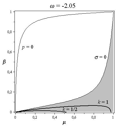
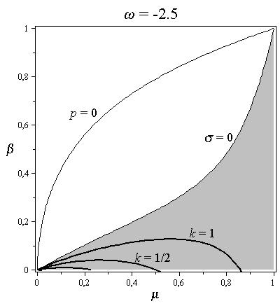
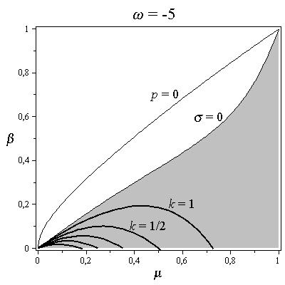
Figure 1: Contour plots for $\sigma(\mu,\beta,\omega_{0})$ and $p(\mu,\beta,\omega_{0})$ for $\omega_{0}=-2.05$, $-2.5$, and $-5$. Thin solid curves denote lines of zero level: $\sigma(\mu,\beta,\omega_{0})=0$ (lower line) and $p(\mu,\beta,\omega_{0})=0$ (upper line). A corresponding value is positive in the region below the zero level line, and so both $\sigma>0$ and $p>0$ in the shadowed region. Thick solid curves denote lines given by the equation of state $p(\mu,\beta,\omega_{0})-k\sigma(\mu,\beta,\omega_{0})=0$, where $k=1,\frac{1}{2},\frac{1}{3},\frac{1}{4},\frac{1}{5}$ from top to down.

Additionally, any reasonable model of matter should include an equation of state $p=p(\sigma)$ imposing some relation between the energy density $\sigma$ and the pressure $p$. Hereafter we will consider the barotropic equation of state $p=k\sigma$. Note that the equation-of-state parameter $k$ is non-negative, $k\geq 0$, for ordinary matter with positive energy density and non-negative pressure. Moreover, the condition $k\leq 1$ guarantees that the speed of sound in matter medium does not exceed the speed of light. In particular, $k=0$ for the dust, $k=1/3$ for the radiation, $k=1$ for the stiff matter. By using Eqs. 26, the equation of state can be rewritten as

$$p(\mu,\beta,\omega)-k\sigma(\mu,\beta,\omega)=0.$$ (27)

For given $\omega$ and $k$ this equation provides an additional relation between $\mu$ and $\beta$ which can be graphically represented as a some curve on the $(\mu,\beta)$-plane. In Fig. 1 we show such curves given for different values of $\omega$ and $k$. The graphical representation illustrates that for any $\omega<-2$ and $k>k_{min}(\omega)$, there exist a domain of $(\mu,\beta)$, where $\mu\in(0,\mu_{max}(\omega,k))$ and $\beta\in(0,\beta_{max}(\omega,k))$, such that the equation of state 27 holds. Note that a boundary value $k_{min}$ depends on $\omega$, and $\mu_{max}$ and $\beta_{max}$ depend both on $\omega$ and $k$. Note also that since $k_{min}(\omega)>0$, then $p>0$, and so matter filling the thin shell is not the dust with zero pressure.

Finally, we may conclude that the thin shell dividing two static spherically symmetric regions with different Brans-Dicke vacua can be made from ordinary matter. In particular, it can be the perfect fluid with the barotropic equation of state.

IV Composite configuration with a wormhole

In previous sections we have constructed the static spherically symmetric configuration composed of two Brans-Dicke vacua and demonstrated that the thin shell dividing the regions with different vacua can be made from ordinary matter. In this section we will discuss the problem: Under which conditions does the composite configuration represent a wormhole?

The exterior region of the composite configuration is described by the Schwarzschild metric and does not contain any wormholes. Let us consider the interior region. The interior metric 10 has an explicit singular behavior at $r=B$. To determine either it is a real or fictitious (coordinate) singularity, we should explore a behavior of curvature invariants. For example, the scalar curvature calculated in the metric 10 reads

$$R=-\frac{8e^{-2\lambda_{0}}r^{4}B^{2}(A^{2}-C^{2}-C-1)}{A^{2}(r-B)^{2(2A-C-1)/A}(r+B)^{2(2A+C+1)/A}}.$$ (28)

It is obvious that $R$ becomes to be singular in points where the denominator of Eq. 28 is equal to zero. In particular, if the power of the term $(r-B)^{2(2A-C-1)/A}$ is positive then $r=B$ is a naked singularity. And vice versa, the scalar curvature $R$ remains being regular at $r=B$ provided the power of $(r-B)^{2(2A-C-1)/A}$ is negative. Substituting $C(\omega)$ and $A(\omega)$ given by Eqs. 8 and 25 into the inequality $2(2A-C-1)/A<0$ we obtain

$$2-\frac{\omega+1}{\omega+2}\sqrt{\frac{2\omega+4}{2\omega+3}}<0.$$ (29)

The last inequality is fulfilled in a narrow interval

$$-2-\frac{\sqrt{3}}{3}<\omega<-2.$$ (30)

Hence the scalar curvature $R$ is regular at $r=B$ if and only if $\omega$ takes its value within the interval 30. Moreover, since $R\propto(r-B)^{2|2A-C-1|/A}$, it is equal to zero at $r=B$. Note that in this case the metric function $e^{2\lambda_{int}(r)}$ given by Eq. 10b tends to infinity as $r\to B$, and hence $r=B$ is a flat spacial infinity.

Finally, the composite vacuum configuration with $-2-\frac{\sqrt{3}}{3}<\omega<-2$ is regular in the range $r\in(B,\infty)$, does not contain horizons in this range, and is asymptotically flat both as $r\to B$ and $r\to\infty$. Therefore, we can conclude that such the configuration is nothing but a wormhole.

Let us determine a position of the wormhole throat. It corresponds to a sphere $r=r_{th}$ with the radius $r_{th}$ providing a global minimum of the function $r^{2}e^{2\lambda_{int}(r)}$ (this guarantees the minimality of area of the sphere). The value $r_{th}$ is called a throat radius. Taking into account Eq. 10b, we find

$$r_{th}=B\left[\frac{C+1}{A}+\sqrt{\left(\frac{C+1}{A}\right)^{2}-1}\right].$$ (31)

Substituting Eqs. 8 and 25 for $C(\omega)$ and $A(\omega)$ into the last expression yields

$$r_{th}=B\gamma(\omega),$$ (32)

where

$$\gamma(\omega)=\frac{\omega+1}{\omega+2}\sqrt{\frac{2\omega+4}{2\omega+3}}+\sqrt{\frac{-3\omega-4}{(2\omega+3)(\omega+2)}}.$$

One can easily check that $\gamma(\omega)>1$ for any $\omega<-2$, and hence $r_{th}>B$.

Since $B=a\beta$, we have $r_{th}=a\beta\gamma(\omega)$. As was shown in the previous section, if the thin shell is made from the perfect fluid with the barotropic equation of state $p=k\sigma$, then $\beta<\beta_{max}(\omega,k)$. A numerical analysis shows that $\beta_{max}(\omega,k)\gamma(\omega)<1$ for any $\omega<-2$ and $k>k_{min}(\omega)$, and so $r_{th}<a$. Therefore, we can conclude that the wormhole throat $r=r_{th}$ is situated within the interior region $r\in(B,a)$ of composite vacuum configuration.

V Summary

In this paper we have constructed a new static spherically symmetric configuration composed of interior and exterior Brans-Dicke vacua divided by thin matter shell. Both vacua correspond to the same Brans-Dicke coupling parameter $\omega$, however they are described by the Brans class I solution 3 with different sets of parameters of integration. In particular, the exterior vacuum solution has $C_{ext}(\omega)\equiv 0$. In this case the Brans class I solution with any $\omega$ just reduces to the Schwarzschild one being consistent with restrictions on the post-Newtonian parameters following from recent Cassini data. The interior region possesses a strong gravitational field, and so, generally, $C_{int}(\omega)\not=0$. In particular, we have used a specific choice $C(\omega)=-1/(\omega+2)$. In this case the Brans class I solution describes a wormhole provided $\omega$ lies in the narrow interval $-2-\frac{\sqrt{3}}{3}<\omega<-2$. The interior and exterior regions are matched at a thin shell made from ordinary matter with positive energy density and pressure. We have studied in detail the shell made from a perfect fluid with the barotropic equation of state $p=k\sigma$ with $0\leq k\leq 1$. The resulting configuration represents a composite wormhole, i.e. the thin matter shell with the Schwarzschild-like exterior region and the interior region containing the wormhole throat.

An interesting feature of composite wormholes is that the strong-field interior region containing all exotic ghost-like matter is hidden behind the matching surface, whereas the weak-field region out of it possesses the usual Schwarzschild vacuum. Such the configuration is similar to the model of trapped-ghost wormholes BroSus . Note that in both models wormholes are twice asymptotically flat. However, in the trapped-ghost wormhole model the ghost is hidden in some restricted region around the throat, whereas in the composite wormhole model the ghost-like Brans-Dicke scalar occupies the “half” of wormhole spacetime behind the matching surface. Anyway, in the composite wormhole configuration a ghost is hidden in the strong-field interior region, which may in principle explain why no ghosts are observed under usual conditions.

References

- (1) C. M. Will, Theory and Experiment in Gravitational Physics (Cambridge, Cambridge University Press, 1993).
- (2) C. Brans and R. H. Dicke, Phys. Rev. 124, 925 (1961).
- (3) C. H. Brans, Phys. Rev. 125, 2194 (1962).
- (4) Y. Fujii, N. Maeda, The scalar-tensor theory of gravitation (Cambridge, Cambridge University Press, 2003).
- (5) A. Agnese and M. La Camera, Phys. Rev. D 51, 2011 (1995).
- (6) K. K. Nandi, A. Islam, and J. Evans, Phys. Rev. D 55, 2497 (1997).
- (7) L. A. Anchordoqui, A. G. Grunfeld, D. F. Torres, Grav. Cosmol. 4, 287 (1998).
- (8) K. K. Nandi, B. Bhattacharjee, S. M. K. Alam and J. Evans, Phys. Rev. D 57, 823 (1998).
- (9) A. Bhadra, K. Sarkar, Mod. Phys. Lett. A20, 1831 (2005).
- (10) F.S.N. Lobo and M.A. Oliveira, Phys. Rev. D 81, 067501 (2010).
- (11) K.A. Bronnikov, M.V. Skvortsova, A.A. Starobinsky, Grav. Cosmol. 16, 216 (2010).
- (12) A. Bhadra and K. Sarkar, Gen. Rel. Grav. 37, 2189 (2005).
- (13) B. Bertotti, L. Iess, P. Tortora, Nature 425, 374 (2003).
- (14) Will, C. M., (2006) The Confrontation between General Relativity and Experiment, http://relativity.livingreviews.org/ Articles/lrr-2006-3/
- (15) S. Weinberg, Gravitation and Cosmology (Wiley, New York,1972)
- (16) A. Bhadra and K. K. Nandi, Phys.Rev. D 64, 087501 (2001).
- (17) C. Romero and A. Barros, Phys.Lett. A173, 243 (1993).
- (18) N. Banerjee and S. Sen, Phys.Rev. D 56,1334 (1997).
- (19) V. Faraoni,Phys.Rev.D 59, 084021 (1999).
- (20) A. Bhadra, arXiv:gr-qc/0204014.
- (21) T. Matsuda, Prog. Theor. Phys. 47, 738 (1972).
- (22) E. F. Eiroa, M. G. Richarte, C. Simeone, Phys.Lett. A373 (2008) 1-4; Erratum-ibid. A373 (2009) 2399-2400.
- (23) X. Yue, S. Gao, Phys. Lett. A375, 2193 (2011).
- (24) M. Visser, Phys. Rev. D 39, 3182 (1989).
- (25) M. Visser, Nucl. Phys. B 328, 203 (1989).
- (26) A. P. Lightman, W. H. Press, R. H. Price, S. A. Teukolsky, Problem book in relativity and gravitation (Princeton, Princeton University Press, 1975).
- (27) N. Sen, Ann. Phys. (Leipzig) 73, 365 (1924); K. Lanczos, ibid. 74, 518 (1924); G. Darmois, M emorial des Sciences Math ematiques, Fascicule XXV, Chap. V (Gauthier-Villars, Paris, 1927); W. Israel, Nuovo Cimento 44B, 1 (1966); ibid. 48B, 463(E) (1967).
- (28) K.G. Suffern, J. Phys. A: Math. Gen. 15, 1599 (1982); C. Barrab‘es and G.F. Bressange, Class. Quantum Grav. 14, 805 (1997); F. Dahia and C. Romero, Phys. Rev. D 60, 104019 (1999).
- (29) K. A. Bronnikov and S. V. Sushkov, Class. Quant. Grav. 27, 095022 (2010).