Generalized Master equation approach to mesoscopic time-dependent transport

Abstract

We use a generalized Master equation (GME) formalism to describe the non-equilibrium time-dependent transport through a short quantum wire connected to semi-infinite biased leads. The contact strength between the leads and the wire are modulated by out-of-phase time-dependent functions which simulate a turnstile device. One lead is fixed at one end of the sample whereas the other lead has a variable placement. The system is described by a lattice model. We find that the currents in both leads depend on the placement of the second lead. In the rather small bias regime we obtain transient currents flowing against the bias for short time intervals. The GME is solved numerically in small time steps without resorting to the traditional Markov and rotating wave approximations. The Coulomb interaction between the electrons in the sample is included via the exact diagonalization method.

1 Introduction

The theoretical description of time-dependent transport in semiconductor nanostructures has received considerable attention in the last few years. Non-equilibrium Greens’ function techniques and density-functional methods were developed for transient current calculations in interacting and non-interacting structures (see [1, 2, 3, 4] and references therein). These methods were employed to study the response of a mesoscopic sample to a time-dependent (possibly pulsed) voltage applied on the leads and/or to check the expected crossover to a steady-state.

A strong motivation behind these studies is the need to model and predict the transient response of open and interacting nanodevices subjected to time-dependent signals. Since in real systems both the contacts and sample geometry as well as the charging and correlation effects are important, the numerical implementation of the various formal methods requires extensive and costly computational work.

Recently we reported transport calculations for a two-dimensional parabolic quantum wire in the turnstile setup [5], where the Coulomb interaction between electrons was neglected. The wire was in contact with external leads, seen as particle reservoirs, and the contact regions were described by a phenomenological ansatz. We provided a careful analysis of the electronic propagation on the edge states that develop in the presence of a strong perpendicular magnetic field. Let us remind here that the turnstile setup was experimentally realized by Kouwenhoven et al. [6]. It essentially involves a time-dependent modulation (pumping) of the tunneling barriers between the finite sample and drain and source leads, respectively. During the first half of the pumping cycle the system opens only to the source lead whereas during the second half of the cycle the drain contact opens. At certain parameters an integer number of electrons is transferred across the sample in a complete cycle. Similar transient current measurements were performed in a pump-and-probe configuration [7, 8, 9]. More complex turnstile pumps have been studied by numerical simulations, like one-dimensional arrays of junctions [10] or two-dimensional multidot systems [11]. The turnstile regime differs from the adiabatic quantum pumping where charge is transferred along a sample even in the absence of a bias.

In this paper we describe the turnstile regime of a one-dimensional (1D) quantum wire (“the sample”). The effect of the electron-electron interaction is included in the sample via the exact diagonalization method while the time-dependent transport is performed within the generalized Master equation (GME) formalism as it is described in Ref. [12]. The implemented GME formalism can be used to describe both the initial transient regime immediately after the coupling of the leads to the sample and the evolution towards a steady state achieved in the long time limit. To the best of our knowledge these are the first numerical simulations of electronic transport through a Coulomb interacting and spatially extended quantum turnstile. We discuss for the first time the effect of contacts’ location on the transient currents. More precisely, we show that if the drain lead is attached to different regions of the quantum wire the currents in both leads are considerably affected.

The paper is organized as follows: The model and the methodology are described in Section 2, the numerical results are presented in Section 3, and the conclusions in Section 4.

2 The physical model and the GME

2.1 Setup

The physical system consists in a sample connected to two leads acting as particle reservoirs. We shall adopt a tight-binding description of the system: the sample is a 10-site quantum wire and the leads are 1D and semi-infinite. A sketch is given in Fig. 1. The left lead (or the source, marked as $L$) is contacted at one end of the sample and the right lead (or the drain, marked as $R$) may be contacted on any other site. The Hamiltonian of the coupled and electrically biased system reads as

$$H(t)=\sum_{\ell}H_{\ell}+H_{S}+H_{T}(t)=H_{0}+H_{T}(t)\,,$$ (1)

where $H_{S}$ is the Hamiltonian of the isolated sample, including the electron-electron interaction, and $H_{\ell}$, with $\{\ell\}=(L,R)$, corresponds to the left and the right leads. $H_{T}$ describes the time-dependent coupling between the single-particle basis states $\{|\phi_{n}\rangle\}$ of the isolated sample and the states $\{{\psi}_{q\ell}\}$ of the leads:

$$H_{T}(t)=\sum_{n}\sum_{\ell}\int\mathrm{d}q\>\chi_{\ell}(t)(T^{\ell}_{qn}c^{\dagger}_{q\ell}d_{n}+h.c.)\,.$$ (2)

The function $\chi_{\ell}(t)$ describes the time-dependent switching of the sample-lead contacts, while $d^{\dagger}_{n}$ and $c_{q\ell}$ create/annihilate electrons in the corresponding single-particle states of the sample or leads, respectively. The coupling coefficient $T^{\ell}_{qn}=V_{0}{\psi}^{*}_{q\ell}(0)\phi_{n}(i_{\ell})$ involves the two eigenfunctions evaluated at the contact sites $(0,i_{\ell})$, $0$ being the site of the lead $\ell$ and $i_{\ell}$ the site in the sample [12]. In our present calculations we keep the left lead connected to the site $i_{L}=1$, while the position of the right lead is $i_{R}=10$ or $i_{R}=3$. The parameter $V_{0}$ plays the role of a coupling constant between the sample and the leads.

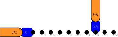
Figure 1: A sketch of the system under study. A 1D lattice with 10 sites (“the sample”) is connected to two semi-infinite leads via tunneling. The left lead is connected to the left end of lattice, while the position of the right lead can be changed. The contacts are modulated in time with the functions $\chi_{L,R}$ given in Eq. 5.

2.2 GME

Following the Nakajima-Zwanzig technique [13] we define the reduced density operator (RDO), $\rho(t)$, by tracing out the degrees of freedom of the environment, the leads in our case, over the statistical operator of the entire system, $W(t)$:

$$\rho(t)=\tr_{L}\tr_{R}W(t)\,,\quad\rho(0)=\rho_{S}\,.$$ (3)

The initial condition corresponds to a decoupled sample and leads when the RDO is just the statistical operator of the isolated sample $\rho_{S}$. For a sufficiently weak coupling strength ($V_{0}$) one obtains the non-Markovian integro-differential Master equation for the RDO:

$${\dot{\rho}}(t)=-\frac{i}{\hbar}[H_{S},\rho(t)]-\frac{1}{\hbar^{2}}\sum_{\ell}\int\mathrm{d}q\>\chi_{\ell}(t)([{\cal T}_{q\ell},\Omega_{q\ell}(t)]+h.c.)\,,$$

where the operators $\Omega_{q\ell}$ and $\Pi_{q\ell}$ are defined as

$$\Omega_{q\ell}(t)=e^{-itH_{S}}\int_{0}^{t}\,\mathrm{d}s\>\chi_{\ell}(s)\Pi_{q\ell}(s)e^{i(s-t)\varepsilon_{q\ell}}e^{itH_{S}}\,,$$

$$\Pi_{q\ell}(s)=e^{isH_{S}}\left({\cal T}_{q\ell}^{\dagger}\rho(s)(1-f_{\ell})-\rho(s){\cal T}_{q\ell}^{\dagger}f_{\ell}\right)e^{-isH_{S}}\,,$$

and $f_{\ell}$ is the Fermi function of the lead $\ell$. The operators ${\cal T}_{q\ell}$ and ${\cal T}_{q\ell}^{\dagger}$ describe the ’transitions’ between two many-electron states (MES) $|\alpha\rangle$ and $|\beta\rangle$ when one electron enters the sample or leaves it:

$$\left({\cal T}_{q\ell}\right)_{\alpha\beta}=\sum_{n}T^{\ell}_{qn}\langle\alpha|d^{\dagger}_{n}|\beta\rangle\,.$$ (4)

The GME is solved numerically by calculating the matrix elements of the RDO in the basis of the interacting MES, in small time steps, following a Crank-Nicolson algorithm. Using the RDO we obtain the time dependent charge and currents in the system. More details can be found in Ref. [12].

2.3 Coulomb interaction

We will ignore the Coulomb effects in the leads, where we assume a high concentration of electrons and thus strong screening and fast particle rearrangements. The Coulomb electron-electron interaction is considered in detail only in the sample, where Coulomb blocking effects may occur. We calculate the MES in the sample following the exact diagonalization method, i. e. without any mean field approximation. The interacting MES are calculated in the Fock space as superpositions of non-interacting MES derived from Slater determinants [12]. Since the sample is open the number of electrons is not fixed, but the Coulomb interaction conserves the number of electrons. With 10 lattice sites we obtain 10 single-particle eigenstates and thus $2^{10}=1024$ elements in the Fock space spanned by the occupation numbers. The Coulomb effects are measured by the ratio of a characteristic Coulomb energy $U_{C}=e^{2}/(\kappa a)$ and the hopping energy $t_{s}=\hbar^{2}/(2m_{eff}a^{2})$. Here $a$ denotes the inter-site distance (the lattice constant of the discretized system), while $\kappa$ and $m_{eff}$ are material parameters, the dielectric constant and the electron effective mass, respectively. In our calculations the relative strength of the Coulomb interaction, $u_{C}=U_{C}/t_{s}$. is considered a free parameter. We will use $u_{C}=0.5$. For a material like GaAs this value would correspond to a sample length of $9a\approx 22$ nm. This length may not look very realistic, but the choice of the parameters was determined by the computational time spent in solving the GME which grows very fast with the number of MES.

The chemical potentials in the leads create a bias window $\Delta\mu=\mu_{L}-\mu_{R}$. The MES of the sample which participate in the transport correspond to chemical potentials $\mu_{N}^{(i)}:={\cal E}_{N}^{(i)}-{\cal E}_{N-1}^{(0)}$ situated within the bias window, or maybe only slightly outside, depending on the sample-leads coupling constant $V_{0}$ [12]. Here ${\cal E}_{N}^{(i)}$ is an energy of the sample spectrum containing $N$ particles, $i=0$ indicating to the ground state and $i>0$ the excited states. A diagram of the chemical potentials is shown in Fig. 2.

2.4 Time-dependent switching

The switching-functions in Eq. 2 act on the contact regions shaded blue in Fig. 1 and are used to mimic potential barriers with time dependent height. In the present study they are made by combining two quasi Fermi functions that are shifted relatively to each other,

$$\chi_{\ell}(t)=1-\frac{1}{e^{t-\gamma_{s}^{\ell}-\delta}+1}-\frac{1}{e^{-(t-\gamma_{s}^{\ell})+(T_{p}^{\ell}+\delta)}+1}\,,\qquad t\in[0,\,2T_{p}^{\ell}]\,,$$ (5)

where $\gamma_{s}^{\ell}=\{0,\,T_{p}^{L}\}$ defines the phase shift between the leads ($\ell=L,R$) and $T_{p}^{\ell}=30$ is the pulse length, the same in the two leads. The parameter $\delta$ controls the shape of the pulse and is fixed at the value $\delta=10$. The time unit used is $\hbar/t_{s}$. The time dependent contact functions are graphed at the bottom of Fig. 3. The initial values are $\chi_{L,R}(0)=0$, i. e. the leads and the sample are initially disconnected.

3 Results

We chose the bias window $\Delta\mu=\mu_{L}-\mu_{R}$ to include the ground state with $N=3$ electrons. We performed transport calculations for two bias windows: a larger one, with $\mu_{L}=3.30$ and $\mu_{R}=2.90$, and a narrower one, with $\mu_{L}=3.20$ and $\mu_{R}=2.98$, as indicated also in Fig. 2. In addition, we also collected the results at vanishing bias $\mu_{L}=\mu_{R}=3.20$.

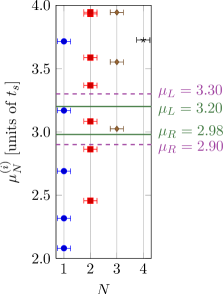
Figure 2: The $\mu$-diagram vs. the number of particles $N$ for $u_{C}=0.5$. The blue points correspond to single-particle states, the red points to two-particle states, the brown points to three-particle states, and the only black point to four particles. The bias window is $\Delta\mu=\mu_{L}-\mu_{R}$. The small bias window is $\Delta\mu=3.20-2.98=0.22$ (green). The large one is $\Delta\mu=3.30-2.90=0.40$ (violet). Both bias windows include the ground state of three particles, but also excited one and two-particle states. So the expected number of electrons in the steady state is slightly below three.

We start the time-dependent calculations with $N=3$ electrons in the sample, initially in the ground state. We place the left lead ($L$) in contact with site 1 of the sample (the left end) and the right lead ($R$) in two different locations: first on site 10 (the right end) and then on site 3. In each case we turn on the turnstile, i. e. $\chi_{L,R}(t)$ follow Eq. (5), and calculate the time dependent charge in the sample and the currents in the left and right leads. In Fig. 3 we show the evolution of the total charge in the system for the two contact configurations mentioned above and the narrower bias window. The modulating signals impose charge oscillations, which after some time become periodic. Due to the choice of the bias window the dominant populations correspond to the three particle ground state and to a two-particle excited state. Single particle states are practically unpopulated and inactive in this case. We see that the charge accumulated in the sample ’feels’ the different placements of the right lead. Indeed, when the drain lead is coupled to the site 3 the oscillations of the total charge diminish compared to the case when the drain is on site 10. One can say that part of the charge located beyond the right contact, i. e. between sites 3 and 10, is somehow frozen and does not contribute to transport. Note however than in both configurations the populations of the two-particle and three-particle states have opposite variations in time, i. e. the gain of one is partly compensated by the loss of the other one.

The same behavior can be observed in the charge distribution along the sample, which is shown in Fig. 4 at a particular time moment. The charge distribution is far from being homogeneous, less charge being localized at the edges of the wire than in the center. The charge distribution is also not symmetric along the sample, and at each site it oscillates in time with frequencies related to the charging times of the active MES. Consequently the currents in the leads also oscillate in time within each pumping period.

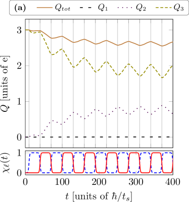
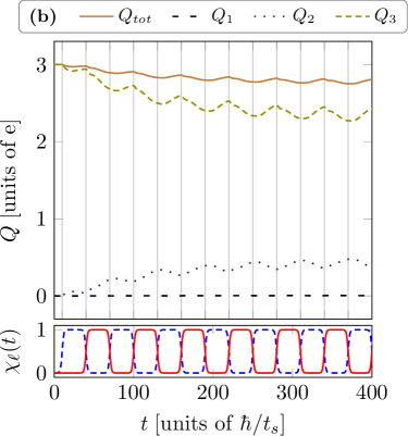
Figure 3: The time dependent charge for $\mu_{L}=3.20$, $\mu_{R}=2.98$. The contact functions $\chi_{L,R}$, given by Eq. 5, are shown at the bottom. (a) Left lead at site 1 (blue), right lead at site 10 (red). (b) Left lead at site 1, right lead at site 3. The total charge is shown by the continuous brown line. The dashed lines show the population of the states with 1, 2, and 3 electrons (indicated as $Q_{1}$, $Q_{2}$ and $Q_{3}$ on the top of the figures).

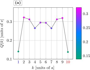
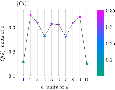
Figure 4: A snapshot of the charge distribution along the 10 sites, for $\mu_{L}=3.20$, $\mu_{R}=2.98$. The time is $t=400$. The position of the right contact is shown on the horizontal axis in red. (a) Left 1 Right 10. (b) Left 1 Right 3.

In the next figures we show the calculated currents in the two leads. In Fig. 5 we show the time dependent currents for zero bias. The oscillations of the currents within each cycle average practically to zero, so we can say that no net charge is transferred through the sample. The positive values of the currents correspond to the direction $L\to R$ and the negative values to the opposite direction, $R\to L$. One can notice some differences in the current oscillations between the two placements of the right contacts, on site 10 and on site 3, respectively. More and sharper oscillations of the currents occur in the later case, but still one can say that qualitatively the currents look similar in the two cases.

This situation changes totally with increasing the bias window. In the next figure, 6, we show the currents for the small bias window, i. e. $\mu_{L}=3.20$ and $\mu_{R}=2.98$. Now the current profiles for the two placements of the right contact are qualitatively different. With the right lead on site 10 we obtain positive currents in both leads, describing charge flow in the direction imposed by the the bias, i. e. from the left to the right of the system. Moreover, the current in the left leads partially resembles the pulse shape. But for the other placement, i. e. with the right contact at site 3, we see much stronger oscillations, and even negative currents in both leads for short times. These negative currents are actually against the bias. In spite on their rather small amplitude one should note that these negative currents do not vanish in the long time limit, that is when the evolution of the system is periodic in time. Another particular feature of the asymmetric contact geometry is that it leads to pronounced spikes in the left lead current.

We then increase the bias window and obtain the results shown in Fig. 7. The current pulses in the contact placement $L1-R10$ do not change qualitatively from the previous case of the smaller bias window, but those for the placement $L1-R3$ do change: the negative currents occur only in the right lead (the red solid line), but not in the left lead (the blue dashed line). In this case some charge bounces back an forth between the sites 3 and 10, and enter or exit the sample through the $R$ lead, but it does not reach the $L$ lead at site 1. In other words the placement of the right contact is qualitatively important for the current profiles for a finite bias window. As we have checked, the negative currents survive for a longer period of the pulses.

It is interesting to compare the current in one lead to the time derivative of the charge, Figures 6 and 3. In the simplest interpretation, when the left contact is open and the right contact is closed the charge in the sample increases, and so the left current is positive and the right current is zero. In the next phase, when the left contact closes and the right one opens, the charge decreases, and the right current is positive, the left current being now zero. The charging or discharging are actually complex processes, because different states are occupied with different time constants, and thus the charging is not constant in time, and the currents have oscillations, more or less following the time derivative of the charge. The fine structure of the currents is however more complicated, also related to the charge oscillations on the particular site where the contact is attached.

Finally, we want to comment on the Coulomb effects. The Coulomb interaction which is included in the present calculations has an important role in the charge distribution, through Coulomb blocking and correlation effects, and so the currents are also affected. However, it is quite difficult to compare the results without and with the Coulomb interaction included. If Coulomb effects are neglected ($u_{C}=0$) the whole energy spectrum changes and new states are present within the bias window. Then the chemical potentials in the leads have to be shifted accordingly in order to capture in the bias window states with similar number of electrons as in the interacting case. This means one cannot compare the two situations just by changing only one parameter.

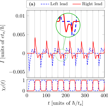
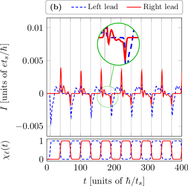
Figure 5: The currents in the two leads at zero bias, $\mu_{L}=\mu_{R}=3.20$: (a) Left 1 Right 10. (b) Left 1 Right 3. At $t=0$ the sample contains three electrons in the ground state.

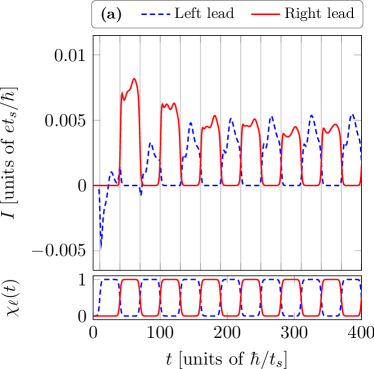
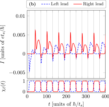
Figure 6: $\mu_{L}=3.20$, $\mu_{R}=2.98$. The currents in the two leads: (a) Left 1 Right 10. (b) Left 1 Right 3. The initial condition corresponds to three electrons in the ground state.

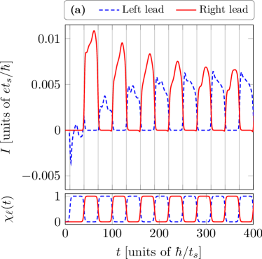
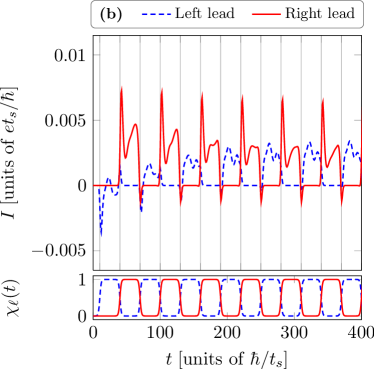
Figure 7: $\mu_{L}=3.30$, $\mu_{R}=2.90$. The currents in the two leads: (a) Left 1 Right 10. (b) Left 1 Right 3. The initial condition corresponds to three electrons in the ground state.

4 Concluding remarks

Using a lattice model we have simulated the time dependent transport through a one-dimensional finite quantum wire attached to two leads. Out-of-phase time-dependent signals are applied at the contact regions, generating a turnstile device. The calculations are performed by solving the generalized Master equation of the reduced density operator. The latter acts in the Fock space of the many-body states of the electrons in the sample, which are calculated via exact diagonalization. We show that the location of the contacts with the leads along the sample leaves clear fingerprints on the transient currents. In particular, when changing the location of the drain lead the currents may flow against the bias for a short time. Even though the currents calculated in these examples are small and we are limited here only to the qualitative effects, the observed counterflow may be seen in future experiments. One can also expect that a suitable placement of the source and drain leads along the sample would be a way to deliver modulated output currents with a desired shape and period.

This work was financially supported by the Icelandic Research Fund.

References

- [1] Kurth S, Stefanucci G, Almbladh C O, Rubio A and Gross E K U 2005 Phys. Rev. B 72(3) 035308
- [2] Stefanucci G and Almbladh C O 2004 Phys. Rev. B 69(19) 195318
- [3] Myöhänen P, Stan A, Stefanucci G and van Leeuwen R 2009 Phys. Rev. B 80(11) 115107
- [4] Myöhänen P, Stan A, Stefanucci G and van Leeuwen R 2010 J. Phys.: Conf. Series 220 012017
- [5] Gainar C M, Moldoveanu V, Manolescu A and Gudmundsson V 2011 New. J. Phys. 13 013014
- [6] Kouwenhoven L P, Johnson A T, van der Vaart N C, Harmans C J P M and Foxon C T 1991 Phys. Rev. Lett. 67(12) 1626–1629
- [7] Fujisawa T, Austing D G, Tokura Y, Hirayama Y and Tarucha S 2003 J. Phys. Cond. Mat. 15 R1395
- [8] Lai W T, Kuo D M and Li P W 2009 Physica E 41 886 – 889
- [9] Naser B, Ferry D K, Heeren J, Reno J L and Bird J P 2007 Appl. Phys. Lett. 90 043103
- [10] Mizugaki Y 2003 J. Appl. Phys 94 4480–4484
- [11] Ikeda H and Tabe M 2006 J. Appl. Phys 99 073705
- [12] Moldoveanu V, Manolescu A, Tang C S and Gudmundsson V 2010 Phys. Rev. B 81(15) 155442
- [13] Timm C 2008 Phys. Rev. B 77(19) 195416