Optimization of the Neutrino Oscillation Parameters
using Differential Evolution

Abstract

We combine Differential Evolution, a new technique, with the traditional grid based method for optimization of solar neutrino oscillation parameters $\Delta m^{2}$ and $\tan^{2}\theta$ for the case of two neutrinos. The Differential Evolution is a population based stochastic algorithm for optimization of real valued non-linear non-differentiable objective functions that has become very popular during the last decade. We calculate well known chi-square ($\chi^{2}$) function for neutrino oscillations for a grid of the parameters using total event rates of chlorine (Homestake), Gallax+GNO, SAGE, Superkamiokande and SNO detectors and theoretically calculated event rates. We find minimum $\chi^{2}$ values in different regions of the parameter space. We explore regions around these minima using Differential Evolution for the fine tuning of the parameters allowing even those values of the parameters which do not lie on any grid. We note as much as 4 times decrease in $\chi^{2}$ value in the SMA region and even better goodness-of-fit as compared to our grid-based results. All this indicates a way out of the impasse faced due to CPU limitations of the larger grid method.

1 Introduction

The flux of solar neutrino was first measured by Raymond Davis Junior and John N. Bahcall at Homestake in late 1960s and a deficit was detected between theory (Standard Solar Model) and experiment [1]. This deficit is known as the Solar Neutrino Problem. Several theoretical explanations have been given to explain this deficit. One of these is neutrino oscillations, the change of electron neutrinos to an other neutrino flavour during their travel from a source point in the sun to the detector at the earth surface [2]. There was no experimental proof for the neutrino oscillations until 2002 when Sudbury Neutrino Observatory (SNO) provided strong evidence for neutrino oscillations [3]. The exact amount of depletion, which may be caused by the neutrino oscillations, however, depends upon the neutrino’s mass-squared difference $\Delta m^{2}\equiv m^{2}_{2}-m^{2}_{1}$ ($m_{1}$ and $m_{2}$ being mass eigen-states of two neutrinos) and mixing angle $\theta$, which defines the relation between flavor eigen-states and mass eigen-states of the neutrinos, in the interval $[0,\pi/2]$.

The data from different neutrino experiments have provided the base to explore the field of neutrino physics. In the global analysis of solar neutrino data, we calculate theoretically expected event rates with oscillations at different detector locations and combine it with experimental event rates statistically through the chi-square ($\chi^{2}$) function, as defined below by Eq.(1), for a grid of values of the parameters $\mathrm{\Delta m^{2}}$ and $\mathrm{tan^{2}\theta}$. The values of these parameters with minimum chi-square in different regions of the parameter space suggest different oscillation solutions. The names of these solutions, found in the literature, along with specification of the regions in the parameter space are: Small Mixing Angle (SMA: $10^{-4}\leq\mathrm{tan^{2}\theta}\leq 3\times 10^{-2},\,\,3\times 10^{-7}\mathrm{eV^{2}}\leq\mathrm{\Delta m^{2}}\leq 10^{-4}\mathrm{eV^{2}}$), Large Mixing Angle (LMA: $3\times 10^{-2}\leq\mathrm{tan^{2}\theta}\leq 2,\,\,2\times 10^{-6}\mathrm{eV^{2}}\leq\mathrm{\Delta m^{2}}\leq 10^{-3}\mathrm{eV^{2}}$), Low Probability Low Mass (LOW: $3\times 10^{-2}\leq\mathrm{tan^{2}\theta}\leq 2,\,\,10^{-8}\mathrm{eV^{2}}\leq\mathrm{\Delta m^{2}}\leq 2\times 10^{-6}\mathrm{eV^{2}}$) and Vacuum Oscillation (VO: $0.1\leq\mathrm{tan^{2}\theta}\leq 1,\,\,10^{-11}\mathrm{eV^{2}}\leq\mathrm{\Delta m^{2}}\leq 10^{-8}\mathrm{eV^{2}}$) [4]. Extensive work has been done on the global analysis of solar neutrino data [5, 6, 7, 8, 9, 10, 11, 12, 13, 14, 15] and now is the era of precision measurement of the neutrino oscillation parameters [16, 17].

Traditionally, the whole parameter space ($10^{-4}\leq\mathrm{tan^{2}\theta}\leq 10$, $10^{-13}\mathrm{eV^{2}}\leq\mathrm{\Delta m^{2}}\leq 10^{-3}\mathrm{eV^{2}}$) is divided into a grid of points by assigning a variable to each parameter and varying its logarithm uniformly. The chi-square values are calculated for each point in the parameter space either by using $\mathrm{{}^{8}B}$ flux constrained by the Standard Solar Model, e.g., BS05(OP) [18] in our case, or by using unconstrained $\mathrm{{}^{8}B}$ flux [9] where it is varied about the value predicted by the Standard Solar Model. The global minimum chi-square value $\chi^{2}_{min}$ is found and $\mathrm{100\,\beta}\%$ C.L. (Confidence Level) contours are drawn in the $\mathrm{tan^{2}\theta}-\mathrm{\Delta m^{2}}$ plane by joining points with $\chi^{2}=\chi^{2}_{min}+\Delta\chi^{2}$ for different confidence levels. From the chi-square distribution one can easily find that $\Delta\chi^{2}=2.28,4.61,5.99,9.21,11.83$ for 68%, 90%, 95%, 99% and 99.73% C.L. for two degrees of freedom. Minimum chi-square values are found in all the regions and the goodness-of-fit, corresponding to each of the minimum chi-square, is calculated. To find the each goodness-of-fit the chi-square distribution is used and confidence level $\mathrm{100(1-\beta)}\%$, corresponding to the minimum chi-square in the region and the degree of freedom of the analysis, is calculated [4, 9]. In our analysis we used total event rates of chlorine (Homestake), Gallax+GNO, SAGE, Superkamiokande, SNO CC and NC experiments. So the number of degrees of freedom was 4 (6(rates)–2(parameters: $\mathrm{tan^{2}\theta}\,\,\mathrm{and}\,\,\mathrm{\Delta m^{2}}$)).

When we use the Differential Evolution (DE), the parameters are randomly selected in the given range and checked for a decrease of chisquare, in contrast with the traditional grid based method as described in the above paragraph. Thus we selected the vectors with least chi-square values, in different regions of the selected grid, as starting points and used DE for the fine tuning of the parameters by exploring region around the selected vectors in the parameter space.

Here in section 2, we define the chi-square ($\chi^{2}$) function for the solar neutrino oscillations. We use the same $\chi^{2}$ function definition in the algorithm of DE as well as in the traditional method. In section 3, we describe algorithm of Differential Evolution along with its salient features. In section 4 and 5, we describe results of global analysis by grid and those obtained using Differential Evolution respectively. Our conclusions are given in section 6.

2 Chi-square ($\chi^{2}$) Function Definition

In our $\chi^{2}$ analysis, we used the updated data of total event rates of different solar neutrino experiments. We followed the $\chi^{2}$ definition of ref. [19] and included chlorine (Homestake) [20], weighted average of Gallax and GNO [21], SAGE [22], Superkamiokande [23], SNO CC and SNO NC [24] total rates. The expression for the $\chi^{2}$ is given as:

$$\chi^{2}_{\mathrm{Rates}}=\sum_{j_{1},j_{2}=1,6}(R^{th}_{j_{1}}-R^{exp}_{j_{1}})[V_{j_{1}j_{2}}]^{-2}(R^{th}_{j_{2}}-R^{exp}_{j_{2}}),$$ (1)

where $R^{th}_{j}$ is the theoretically calculated event rate with oscillations at detector $j$ and $R^{exp}_{j}$ is the measured rate. For chlorine, Gallax+GNO and SAGE experiments $R^{th}$ and $R^{exp}$ are in the units of SNU (1 SNU=$10^{-36}$ captures/atom/sec) and for Superkamiokande, SNO CC and SNO NC these are used as ratio to SSM Eq.(8) below. $V_{j_{1}j_{2}}$ is the error matrix that contains experimental (systematic and statistical) errors and theoretical uncertainties that affect solar neutrino fluxes and interaction cross sections. For the calculation of the error matrix $V_{j_{1}j_{2}}$ we followed ref. [19] and for updated uncertainties we used ref. [25]. For the calculation of theoretical event rates, using Eqs.(4-7) below, we first found the time average survival probabilities, over the whole year, of electron neutrino $\langle P_{ee}^{k}(E_{\nu})\rangle$ ($E_{\nu}$ is the neutrino energy in MeV) at the detector locations for the $k^{th}$ neutrino source and for the grid of 101 $\times$ 101 values of $\mathrm{\frac{\Delta m^{2}}{E}}$ and $\mathrm{tan^{2}\theta}$ following the prescriptions described in ref. [9]. For the uniform grid interval distribution we used the parameters $\mathrm{\frac{\Delta m^{2}}{E}}$ and $\mathrm{tan^{2}\theta}$ as exponential functions of the variables $x_{1}$ and $x_{2}$ as:

$$\mathrm{\frac{\Delta m^{2}}{E}}=10^{(0.1x_{1}-13)}$$ (2)

and

$$\mathrm{tan^{2}\theta}=10^{-2(2-0.025x_{2})}$$ (3)

so that discrete values of $x_{1}$ and $x_{2}$ from 0 to 100 cover the entire $\mathrm{tan^{2}\theta}-\mathrm{\Delta m^{2}}$ parameter space. We used the expression for the average expected event rate in the presence of oscillation in case of Chlorine and Gallium detectors given as:

$$R_{j}^{th}=\sum_{k=1\,\mathrm{to}\,8}\phi_{k}\int^{E_{max}}_{E^{j}_{th}}dE_{\nu}\lambda_{k}(E_{\nu})[\sigma_{e,j}(E_{\nu})\langle P_{ee}^{k}(E_{\nu})\rangle].$$ (4)

Here $E^{j}_{th}$ is the process threshold for the $j$th detector ($j$=1,2,3 for Homestake, Gallax+GNO and SAGE respectively). The values of energy threshold $E^{j}_{th}$ for Cl, Ga detectors are 0.814, 0.233 MeV respectively [26]. $\phi_{k}$ are the total neutrino fluxes taken from BS05(OP) [18]. For Gallium detector all fluxes contribute whereas for Chlorine detector all fluxes except pp flux contribute. $\lambda_{k}(E_{\nu})$ are normalized solar neutrino energy spectra for different neutrino sources from the sun, taken from refs. [27, 28], and $\sigma_{e,j}$ is the interaction cross section for $\nu_{e}$ in the $j$th detector. Numerical data of energy dependent neutrino cross sections for chlorine and gallium experiments is available from ref. [27]. Event rates of Chlorine [20] and Gallium [21, 22] experiments and those calculated from Eq.(4) directly come in the units of SNU.

Superkamiokande and SNO detectors are sensitive for higher energies, so $\phi_{k}$ are the total $\mathrm{{}^{8}B}$ and hep fluxes for these detectors respectively. The expression of the average expected event rate with oscillations for elastic scattering at SK detector is as below:

$$N_{SK}^{th}=\sum_{k=1,2}\phi_{k}\int^{E_{max}}_{0}dE_{\nu}\lambda_{k}(E_{\nu})\times\{\sigma_{e,j}(E_{\nu})\langle P_{ee}^{k}(E_{\nu})\rangle+\sigma_{\mu,j}(E_{\nu})[1-\langle P_{ee}^{k}(E_{\nu})\rangle]\}.$$ (5)

Here $\sigma_{e}$ and $\sigma_{\mu}$ are elastic scattering cross sections for electron and muon neutrinos that we took from ref. [29].

For the SNO charged-current (CC) reaction, $\nu_{e}d\rightarrow e^{-}pp$, we calculated event rate using the expression:

$$N_{CC}^{th}=\sum_{k=1,2}\phi_{k}\int dE_{\nu}\lambda_{k}(E_{\nu})\sigma_{CC}(E_{\nu})\times\langle P_{ee}^{k}(E_{\nu})\rangle.$$ (6)

Here $\sigma_{CC}$ is $\nu d$ CC cross section of which calculational method and updated numerical results are given in refs. [30] and  [31] respectively.

The expression for the SNO neutral-current (NC) reaction, $\nu_{x}d\rightarrow\nu_{x}\,p\,n\,(x=e,\,\mu,\,\tau)$, event rate is given as:

$$N_{NC}^{th}=\sum_{k=1,2}\phi_{k}\int dE_{\nu}\lambda_{k}(E_{\nu})\sigma_{NC}(E_{\nu})\times(\langle P_{ee}^{k}(E_{\nu})\rangle+\langle P_{ea}^{k}(E_{\nu})\rangle).$$ (7)

Here $\sigma_{NC}$ is $\nu d$ NC cross section and $\langle P_{ea}^{k}(E_{\nu})\rangle$ is the time average probability of oscillation into any other active neutrino. We used updated version of CC and NC cross section data from the website given in ref. [31]. In case of oscillation of the $\nu_{e}$ into active neutrino only, $\langle P_{ee}^{k}(E_{\nu})\rangle+\langle P_{ea}^{k}(E_{\nu})\rangle=1$ and $N_{NC}^{th}$ is a constant.

For Superkamiokande [23] and SNO [24] experiments, the event rates come in the unit of $10^{6}\mathrm{cm^{-2}s^{-1}}$. We converted these rates into ratios to SSM predicted rate. We also calculated theoretical event rates as ratios to SSM predicted rate in order to cancel out all energy independent efficiencies and normalizations [8].

$$R_{j}^{th}=\frac{N_{j}^{th}}{N_{j}^{SSM}}$$ (8)

Here $N_{j}^{SSM}$ ($j$=4,5,6 for SK, SNO CC and SNO NC respectively) is the predicted number of events assuming no oscillations. We used the Standard Solar Model BS05(OP) [18] in our calculations. Theoretical event rates, so calculated, were used in Eq.(1) to calculate the chi-square function for different points in the $\mathrm{tan^{2}\theta}-\mathrm{\Delta m^{2}}$ parameter space.

3 Differential Evolution

Differential Evolution (DE) is a simple population based, stochastic direct search method for optimization of real valued, non-linear, non-differentiable objective functions. It was first introduced by Storn and Price in 1997 [32]. Differential Evolution proved itself to be the fastest evolutionary algorithm when participated in First International IEEE Competition on Evolutionary Optimization [33]. DE performed better when compared to other optimization methods like Annealed Nelder and Mead strategy [34], Adaptive Simulated Annealing [35], Genetic Algorithms [36] and Evolution Strategies [37] with regard to number of function evaluations (nfe) required to find the global minima. DE algorithm is easy to use, robust and gives consistent convergence to the global minimum in consecutive independent trials [32, 38].

The general algorithm of DE [39] for minimizing an objective function carries out a number of steps. Here we summarize the steps we carried out for minimizing the $\chi^{2}$ function defined in section 2. We did optimization of the $\chi^{2}$ function individually for different regions of the parameter space to do one fine tuning in each region. The results of the optimization are reported in the section 5 below.

Step I

An array of vectors was initialized to define a population of size NP=20 with D=2 parameters as

$$\mathrm{\textbf{x}}_{i}=\textit{x}_{j,i}\,\,\,\mathrm{where}\,\,\,\,i=1,2,.....,\texttt{NP}\,\,\,\mathrm{and}\,\,\,j=1,..,\texttt{D}.$$ (9)

The parameters, involved here, are $x_{1}$ and $x_{2}$ of Eqs.(2) and (3) on which $\mathrm{\Delta m^{2}/E}$ and $\mathrm{tan^{2}\theta}$ depend. Upper and lower bounds ($b_{j,U}$ and $b_{j,L}$), individually for different regions of the parameter space described in the introduction section, for the $x$ values were specified and each vector $i$ was assigned a value according to

$$\textit{x}_{j,i}=\mathrm{rand}_{j}(0,1)\cdot(b_{j,U}-b_{j,L})+b_{j,L}$$ (10)

where $\mathrm{rand}_{j}\in[0,1]$ is $j^{th}$ evaluation of a uniform random number generator. The $\chi^{2}$ function was calculated for each vector of the population and the vector with least $\chi^{2}$ function value was selected as base vector $\textbf{x}_{r_{o}}$.

Step II

Weighted difference of two randomly selected vectors from the population was added to the base vector $\textbf{x}_{r_{o}}$ to produce a mutant vector population $\textbf{v}_{i}$ of NP trial vectors. The process is known as mutation.

$$\textbf{v}_{i}=\textbf{x}_{r_{o}}+F\cdot(\textbf{x}_{r_{1}}-\textbf{x}_{r_{2}}).$$ (11)

Here the scale factor $F\in[0,2]$ is a real number that controls the amplification of the differential variation. The indices $r_{1},r_{2}\in[1,\texttt{NP}]$ are randomly chosen integers and are different from $r_{o}$.

Different variants of DE mutation are denoted by the notation ‘DE/x/y/z’, where x specifies the vector to be mutated which can be “rand” (a randomly chosen vector) or “best” (the vector of the lowest $\chi^{2}$ from the current population), y is the number of difference vectors used and z is the crossover scheme. The above mentioned variant Eq.(11) is DE/best/1/bin, where the best member of the current population is perturbed with y=1 and the scheme bin indicates that the crossover is controlled by a series of independent binomial experiments. The two variants, reported in the literature [32, 38], very useful for their good convergence properties, are DE/rand/1/bin

$$\textbf{v}_{i}=\textbf{x}_{r_{1}}+F\cdot(\textbf{x}_{r_{2}}-\textbf{x}_{r_{3}}),$$ (12)

and DE/best/2/bin

$$\textbf{v}_{i}=\textbf{x}_{ro}+F\cdot(\textbf{x}_{r_{1}}+\textbf{x}_{r_{2}}-\textbf{x}_{r_{3}}-\textbf{x}_{r_{4}})\,.$$ (13)

For our problem, we used the variant DE/best/2/bin Eq.(13) for DE mutation, where 2 difference vectors were added to the base vector. The values of $F$ we used are reported in section 5 below.

Step III

The parameters of mutant vector population Eq.(13) were mixed with the parameters of target vectors Eq.(9) in a process called uniform crossover or discrete recombination. After the cross over the trial vector became:

$$\textbf{u}_{i}=\textit{u}_{j,i}=\left\{\begin{array}[]{rr}\textit{v}_{j,i}&\mathrm{If}\,\,(\mathrm{rand}_{j}(0,1)\leq\texttt{Cr}\,\,\mathrm{or}\,\,j=j_{\mathrm{rand}}),\\ \textit{x}_{j,i}&\mathrm{otherwise}.\end{array}\right.$$ (14)

Here $\texttt{Cr}\in[0,1]$ is the cross over probability that controls fraction of the parameters inherited from the mutant population (the values of Cr we used are given in section 5), $\mathrm{rand}_{j}\in[0,1]$ is the output of a random number generator and $j_{\mathrm{rand}}$ $\in[1,2]$ is a randomly chosen index.

Step IV

The $\chi^{2}$ function was evaluated for each of the trial vector $\textbf{u}_{i}$ obtained from Eq.(14). If the trial vector resulted in lower objective function than that of the target vector $\textbf{x}_{i}$, it replaced the target vector in the following generation. Otherwise the target vector was retained. (This operation is called selection.) Thus the target vector for the next generation became:

$$\textbf{x}^{\prime}_{i}=\left\{\begin{array}[]{rr}\textbf{u}_{i}&\mathrm{If}\,\,\chi^{2}(\textbf{u}_{i})\leq\chi^{2}(\textbf{x}_{i}),\\ \textbf{x}_{i}&\mathrm{otherwise}.\end{array}\right.$$ (15)

The processes of mutation, crossover and selection were repeated until the optimum was achieved or the number of iterations (generations) specified in section 5 were completed.

4 Analysis from the Selected Grid

Figure 1 and Table 1 show our best fit oscillation parameters, in different regions, calculated using a grid of 101 $\times$ 101 points of the parameter space. The symbol of star shows the best fit points in the respective regions of the parameter space. Calculations of goodness-of-fit and confidence level are described in the introduction section. We used chi-square function definition of section 2. We used $\mathrm{{}^{8}B}$ flux constrained by the Standard Solar Model BS05(OP). We saw that the point with global minimum or the best fit point in the parameter space lies in the LMA region with $\Delta\mathrm{m^{2}}=2.512\cdot 10^{-5}\mathrm{eV^{2}}$ and $\tan^{2}\theta=3.981\cdot 10^{-1}$ that is consistent with the results found in the literature where SNO data is included in the analysis [9, 10, 12]. Before including the SNO data the best fit was found in the SMA region [26].

A selection of a fine grid with larger number of points in the parameter space, of course, will give better results but limitations of the CPU time restricted us, like others, to a grid with a small number of points. But we point out that even without increasing the number of points in the grid we can get lower $\chi^{2}$ and better g.o.f. by fine tuning of the oscillation parameters using DE. We describe what we mean by fine tuning and report our improvements obtained this way in the next section.

Solution	$\Delta\mathrm{m^{2}}(\mathrm{eV^{2}})$	$\tan^{2}\theta$	$\mathrm{\chi^{2}_{min}}$	g.o.f.
LMA	$2.512\cdot 10^{-5}$	$3.981\cdot 10^{-1}$	0.808	93.77%
VAC	$6.31\cdot 10^{-11}$	$1.00\cdot 10^{0}$	1.268	86.72%
LOW	$1.00\cdot 10^{-8}$	$1.122\cdot 10^{0}$	4.09	39.46%
SMA	$6.31\cdot 10^{-6}$	$1.585\cdot 10^{-3}$	7.78	10.01%

Table 1: Our best-fit values of the oscillation parameters $\Delta\mathrm{m^{2}}$, $\tan^{2}\theta$ along with $\mathrm{\chi^{2}_{min}}$ (4  d.o.f) (6(rates)-2(parameters: $\mathrm{tan^{2}\theta},\mathrm{\Delta m^{2}}$)) and g.o.f. corresponding to Figure 1.

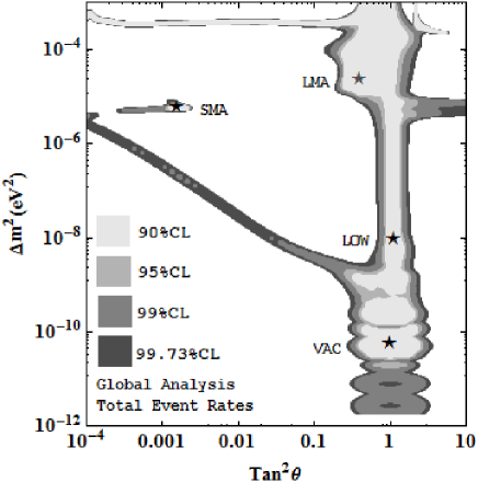
Figure 1: Our global solutions for the total rates. The input data includes total event rates of chlorine [20], weighted average of Gallax and GNO [21], SAGE [22], Superkamiokande [23], SNO CC and SNO NC [24]. The increasing grey level shows 90%, 95%, 99%, 99.73% C.L. Our best-fit points in different regions are marked by stars.

5 Optimization of the Chi-square Function using DE

We have described algorithm of the Differential Evolution in detail in section 3. We wrote the subroutine of the chi-square function, denoted by $\chi^{2}$, following the definition of chi-square in section 2, that depends on $x_{1}$ and $x_{2}$ and used it as objective function of the DE algorithm. We combined the traditional grid-based method with DE in two aspects: First, we used the survival probabilities $\langle P_{ee}^{k}(E_{\nu})\rangle$ already calculated for the discrete values of $x_{1}$ and $x_{2}$ for our grid of 101 $\times$ 101 points of the parameter space and interpolated them to the continuous values of $x_{1}$ and $x_{2}$ to calculate event rates and chi-square function in DE algorithm. We used cubic polynomial fit for the interpolation purpose to fit the data. Second, we used the points with minimum chi-square in different regions of the selected grid Table 1 as the starting points (and members of the respective population array) and explored the space around them for the fine tuning. That is, we searched for the points with smaller $\chi^{2}$ values and better goodness-of-fit of the oscillation parameters.

Solution	Iterations	$\Delta\mathrm{m^{2}}(\mathrm{eV^{2}})$	$\tan^{2}\theta$	$\mathrm{\chi^{2}_{min}}$	$\mathrm{\chi^{2}_{best}}$	g.o.f.
	1-7	$2.51189\cdot 10^{-5}$	$3.98107\cdot 10^{-1}$	0.808314		93.77%
	8-9	$2.50999\cdot 10^{-5}$	$3.97855\cdot 10^{-1}$	0.807316
	10-13	$2.40927\cdot 10^{-5}$	$3.97684\cdot 10^{-1}$	0.804711
	14	$2.49798\cdot 10^{-5}$	$3.97287\cdot 10^{-1}$	0.804564
LMA	15	$2.49307\cdot 10^{-5}$	$3.97028\cdot 10^{-1}$	0.804289
	16	$2.45884\cdot 10^{-5}$	$3.97912\cdot 10^{-1}$	0.804424
	17-21	$2.46633\cdot 10^{-5}$	$3.9751\cdot 10^{-1}$	0.803315
	22-29	$2.43264\cdot 10^{-5}$	$3.98097\cdot 10^{-1}$	0.803192
	30-50	$2.45084\cdot 10^{-5}$	$3.9751\cdot 10^{-1}$	0.802953	0.802953	93.82%
	1	$6.30957\cdot 10^{-11}$	$1.0$	1.26779		86.72%
	2-3	$6.64977\cdot 10^{-11}$	$1.0277$	1.260239
VAC	4-6	$6.70641\cdot 10^{-11}$	$1.01912$	1.25977
	7-43	$6.6423\cdot 10^{-11}$	$0.993134$	1.25948
	44-45	$6.6423\cdot 10^{-11}$	$0.998353$	1.25945
	46-50	$6.70041\cdot 10^{-11}$	$0.99326$	1.25939	1.25939	86.82%
	1-3	$6.30957\cdot 10^{-6}$	$1.58489\cdot 10^{-3}$	7.77933		10.01%
SMA	4	$6.19532\cdot 10^{-6}$	$1.64599\cdot 10^{-3}$	6.24974
	5	$6.10563\cdot 10^{-6}$	$1.48276\cdot 10^{-3}$	5.89341
	6-50	$5.48095\cdot 10^{-6}$	$1.72371\cdot 10^{-3}$	1.86456	1.86456	75.97%
	1	$1.0\cdot 10^{-8}$	$1.12208$	4.18897		39.46%
	2-4	$2.37807\cdot 10^{-8}$	$1.03198$	3.98339
	5-9	$2.95404\cdot 10^{-8}$	$1.03198$	3.97624
LOW	10	$3.3042\cdot 10^{-8}$	$1.03069$	3.97605
	11	$2.80796\cdot 10^{-8}$	$1.02741$	3.9728
	12-20	$3.17357\cdot 10^{-8}$	$1.02741$	3.96267
	21-50	$3.14543\cdot 10^{-8}$	$1.02723$	3.96125	3.96125	41.12%

Table 2: The results of the oscillation parameters during different iterations of the DE algorithm. The improved values of the oscillation parameters $\Delta\mathrm{m^{2}}$, $\tan^{2}\theta$ along with $\mathrm{\chi^{2}_{best}}$ (4 d.o.f) and g.o.f. using Differential Evolution strategy DE/best/2/bin corresponding to Figure 2 are presented. Note in the $1^{st}$ row of different regions, the points with minimum chi-square given in table 1 are taken as first members of the population arrays. The other members of the arrays, for different regions, are selected randomly using DE.

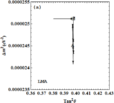
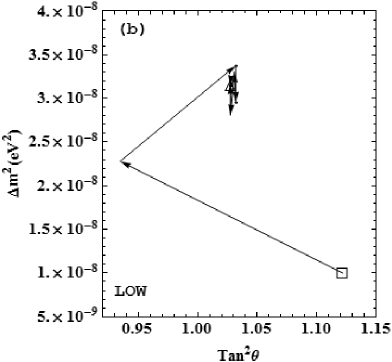
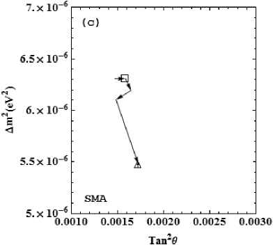
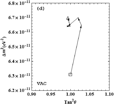
Figure 2: Track of the DE algorithm for optima in different regions using the strategy DE/best/2/bin. The square symbol shows the best point of the 101 $\times$ 101 grid and triangle symbol shows the best point after fine tuning using DE.

In our analysis, the values of DE control variables F and CR were taken as 0.4 and 0.9 respectively for the LMA, SMA and VAC regions. For the LOW region F and CR were both taken as 0.3 for better convergence. Maximum number of iterations were taken to be 50 for all regions. We took the best point in a region of the 101 $\times$ 101 grid in Table 1 as the first member of the population in the first iteration and used the strategy DE/best/2/bin for DE mutation in all the remaining iterations/generations. The steps of DE algorithm, described in section 3, are repeated for the number of iterations specified.

Table 2 and Figure 2 show the results in different regions during and after fine tuning of the oscillation parameters using Differential Evolution. The value of $\mathrm{\chi^{2}_{min}}$ persisted, rejecting all the mutations, for the iterations mentioned in column 2 of Table 2. Accepted mutations resulted in new vectors whose components are given in column 3 and 4 of the following rows. $\mathrm{\chi^{2}_{best}}$ is the minimum chi-square value we obtained in the region specified. In comparison to the results of Table 1, we note here as much as 4 times decrease in the $\chi^{2}_{\mathrm{min}}$ of the SMA region after fine tuning using DE along with a small decrease in all the other regions. Different vectors in Figure 2 show the track of DE algorithm for optima in different regions during iterations specified in Table 2.

6 Conclusions

Fine tuning of the neutrino oscillation parameters using Differential Evolution has been introduced as a solution to the impasse faced due to CPU limitations of the larger grid alternative. We can explore the parameter space deeply due to real nature of the parameters $x_{1}$ and $x_{2}$ using DE in contrast to discrete nature of these parameters in the traditional grid based method. We conclude that combination of Differential Evolution along with traditional method provides smaller chi-square values and better goodness-of-fit of the neutrino oscillation parameters in different regions of the parameter space. We also note a significant change in the results of $\chi^{2}_{\mathrm{min}}$ and g.o.f. in the SMA region after the fine tuning using DE. Even though it is a local decrease, it indicates importance of the exploration of the points within the grid and the efficiency that can be achieved through DE.

References

- [1] J. N. Bahcall, Scientific American, Volume 221, Number 1, July 1969, pp. 28–37.
- [2] L. Wolfenstein, Phys. Rev. D 17, 2369 (1978).
- [3] Q. R. Ahmad et al., Phys. Rev. Lett. 89, 011301 (2002).
- [4] M. V. Garzelli, C. Giunti, Astroparticle Physics 17 (2002) 205–220.
- [5] J. N. Bahcall, P. I. Krastev and A. Yu. Smirnov, Phys. Rev. D 58, 096016 (1998).
- [6] M. C. Gonzalez-Garcia et al., Nuclear Physics B 573 (2000) 3–26.
- [7] M. C. Gonzalez-Garcia and C. Peña-Garay, Nuclear Physics B (Proc. Suppl.) 91 (2001) 80-88.
- [8] M. C. Gonzalez-Garcia and C. Peña-Garay, Phys. Rev. D 63, 073013 (2001).
- [9] J. N. Bahcall, P. I. Krastev and A. Yu. Smirnov, J. High Energy Phys. 05 (2001) 015.
- [10] J. N. Bahcall, M. C. Gonzalez-Garcia and C. Peña-Garay, J. High Energy Phys. 08 (2001) 014.
- [11] P. I. Krastev and A. Yu. Smirnov, Phys. Rev. D 65, 073022 (2002).
- [12] J. N. Bahcall, M. C. Gonzalez-Garcia and C. Peña-Garay, J. High Energy Phys. 07 (2002) 054.
- [13] P. C. de Holanda and A. Yu. Smirnov, Phys. Rev. D 66, 113005 (2002).
- [14] P. Aliani et al., Phys. Rev. D 67, 013006 (2003).
- [15] S. Goswami, A. Bandyopadhyayb and S. Choubey, Nuclear Physics B (Proc. Suppl.) 143 (2005) 121-128.
- [16] P. Yang and Q. Y. Liu, Chin. Phys. Lett. Vol.26 No.3 (2009) 031401.
- [17] P. Yang and Q. Y. Liu, Chin. Phys. Lett. Vol.26 No.8 (2009) 081402.
- [18] J. N. Bahcall, A. M. Serenelli and S. Basu, Astrophys. J. 621 L85 (2005).
- [19] G. L. Fogli and E. Lisi, Astropart. Phys. 3 185 (1995).
- [20] B. T. Cleveland et al., Astrophys. J. 496 505 (1998).
- [21] C. M. Cattadori, Nuclear Physics B (Proc. Suppl.) 110 311-314 (2002).
- [22] J. N. Abdurashitov et al., Phys. Rev. C 80, 015807 (2009).
- [23] K. Abe, Y. Hayato et al., Phys. Rev. D 83, 052010 (2011).
- [24] B. Aharmim, S. N. Ahmed et al., Phys. Rev. Lett. 101, 111301 (2008).
- [25] G. L. Fogli and E. Lisi, Phys. Rev. D 62, 013002 (2001).
- [26] M. C. Gonzalez-Garcia, Yosef Nir, Rev. Mod. Phys. 75 345 (2003).
- [27] J. N. Bahcall et al., Phys. Rev. C 54, 411 (1996); J. N. Bahcall, Phys. Rev. C 56, 3391 (1997).
- [28] J. N. Bahcall and Roger K. Ulrich, Rev. Mod. Phys. 60, 297 (1988); J. N. Bahcall, Phys. Rev. D 49, 3923 (1994).
- [29] J. N. Bahcall et al., Phys. Rev. D 51, 6146 (1995).
- [30] S. Nakamura et al., Phys. Rev. C 63, 034617 (2001); S. Nakamura et al., ibid. 73, 049904(E) (2006);
- [31] S. Nakamura et al., Nuclear Physics A 707, 561–576 (2002).
- [32] R. Storn, K. Price, J. Glob. Optim. 11, 341- 59 (1997).
- [33] K. Price and R. Storn, Procedings of 1996 IEEE International Conference on Evolutionary Computation (ICEC ’ 96), pp. 842 -844 (1996).
- [34] W. H. Press, S. A. Teukolsky, W. T. Vetterling, B. P. Flannery, Numerical recipes in C, Cambridge University Press (1992).
- [35] L. Ingber, Matheml. Comput. Modeling, Vol 18, No. 11, pp 29 -57 (1993).
- [36] D. E. Goldberg, Genetic Algorithms in Search, Optimization and Machine Learning, Addison-Wesley (1989).
- [37] H. P. Schwefel, Evolution and Optimum Seeking, John Wiley (1995).
- [38] P. K. Bergey, C. Ragsdale, Omega 33 255–265 (2005).
- [39] K. V. Price, R. M. Storn, J. A. Lampinen, Differential Evolution: A Practical Approach to Global Optimization, Springer-Verlag Berlin Heidelberg (2005).