Abstract

Effective field theories for quarkonium at zero and finite temperature provide an unifying description for a wide class of phenomena. As an example, we discuss physical effects induced by dipole transitions.

1 Hierarchies

TUM-EFT 23/11

Quarkonia, i.e. heavy quark-antiquark bound states, are systems characterized by hierarchies of energy scales [1]. They follow from the quark mass, $M$, being the largest scale in the system, which, in particular, means that $M\gg p$, the typical momentum transfer in the system, $M\gg\Lambda_{\rm QCD}$, the hadronic scale, and $M\gg\pi T\gg\hbox{other thermal scales}$, where $T$ is the temperature of the medium. These hierarchies allow systematic studies through the construction of suitable effective field theories (EFTs).

(i) The non-relativistic expansion
$M\gg p$ implies that quarkonia are non-relativistic and characterized by the hierarchy of scales typical of a non-relativistic bound state: $p\sim 1/r\sim Mv$ and $E\sim Mv^{2}$, where $r$ is the typical radius, $E$ the typical binding energy and $v\ll 1$ the heavy-quark velocity in the centre-of-mass frame. Note that the hierarchy of non-relativistic scales makes the very difference of quarkonia with heavy-light mesons, which are characterized just by the two scales $M$ and $\Lambda_{\rm QCD}$.

Systematic expansions in the small heavy-quark velocity $v$ may be implemented at the Lagrangian level by constructing suitable non-relativistic effective field theories (EFTs) [2].

(ii) The perturbative expansion
$M\gg\Lambda_{\rm QCD}$ implies $\alpha_{\rm s}(M)\ll 1$: phenomena happening at the scale $M$ may be treated perturbatively. We may further have small couplings if $Mv\gg\Lambda_{\rm QCD}$ and $Mv^{2}\gg\Lambda_{\rm QCD}$, in which case $\alpha_{\rm s}(Mv)\ll 1$ and $\alpha_{\rm s}(Mv^{2})\ll 1$ respectively. Moreover, we have $v\sim\alpha_{\rm s}(Mv)$. This is likely to happen only for the lowest charmonium and bottomonium states, which may be described by weakly-coupled Coulombic bound states, while excited quarkonia probe the transition from Coulombic to confined bound states.

(iii) The thermal expansion
If the temperature of the medium in heavy-ion collisions is such that $M\gg\pi T$, which is the case for most present days colliders, this implies that the quarkonium remains a non-relativistic bound state also in the thermal bath induced by the medium. However, the temperature will, in general, interfere with the other scales of the bound state. As a consequence, bound state observables like masses, lifetimes, decay widths etc. will be modified by the medium. In particular, it is expected that at sufficiently high temperatures the interference of the medium will be such to dissociate the quarkonium. Since different quarkonia have different radii and different binding energies, different quarkonia are expected to dissociate in the medium at different temperatures, providing a thermometer for the plasma [3], see also [4]. $\pi T\gg\hbox{other thermal scales}$ implies a hierarchy also in the thermal scales.

2 Effective field theories

The hierarchies of EFTs for quarkonium at zero and finite temperature are shown in Fig. 1. In the following, we will consider systems for which $Mv\gg T$, so that both the scale $M$ and the scale $Mv$ may be integrated out ignoring medium effects (third column of Fig. 1).

b \put(40.0,0.0){\epsfbox{scalescombT.eps}}

Figure 1: Hierarchies of EFTs for quarkonium at zero temperature [2] and at finite temperature [5, 6, 7, 8, 9].

Heavy quark-antiquark annihilation and production happen at the scale $M$. The suitable EFT is NRQCD [10, 11]. The effective Lagrangian is organized as an expansion in $1/M$ and $\alpha_{\rm s}(M)$:

(1) $${\cal L}_{\rm NRQCD}=\sum_{n}{{c_{n}(\alpha_{\rm s}(M),\mu)\over M^{n}}}\times O_{n}(\mu)\,,$$

where $O_{n}$ are NRQCD operators of dimension $4+n$ and $c_{n}$ are NRQCD matching coefficients. For quarkonium production in NRQCD, see also [12].

The heavy quark and antiquark in quarkonium cannot be resolved at scales lower than $Mv$. The suitable EFT is pNRQCD [13, 14]. The effective Lagrangian is organized as an expansion in $1/M$, $\alpha_{\rm s}(M)$ and $r$:

(2) $${\cal L}_{\rm pNRQCD}=\int d^{3}r\,\sum_{n}\sum_{k}{{c_{n}(\alpha_{\rm s}(M),\mu)\over M^{n}}}\times V_{n,k}(r,\mu^{\prime},\mu)\;r^{k}\times O_{n,k}(\mu^{\prime})\,,$$

where $O_{n,k}$ are pNRQCD operators and $V_{n,k}$ are the pNRQCD matching coefficients. The matching coefficients of the four-fermion, dimension six, operators may be interpreted as the potentials of the bound-state Schrödinger equation, while the matching coefficients of the higher-dimension operators describe the couplings of the heavy quarks to the low-energy degrees of freedom.

Figure 2: Chromoelectric (a), chromomagnetic (b), electric (c) and magnetic (d) dipole interaction vertices. The single line stands for a colour-singlet quark-antiquark propagator, while the double line for a colour-octet quark-antiquark propagator.

To list the low-energy degrees of freedom and to write explicitly the Lagrangian of pNRQCD we need to specify our system. In the following, we will concentrate on the physics of the quarkonium ground states in the presence of a medium whose temperature is much lower than the typical moment transfer in the bound state (this situation includes the vacuum). For a recent review, also on the physics of the quarkonium ground states, we refer to [15]. The suitable EFT for the quarkonium ground states is weakly coupled pNRQCD, since for those systems $Mv\sim M\alpha_{\rm s}\gg Mv^{2}\sim M\alpha_{\rm s}^{2}{\ \lower-1.2pt\vbox{\hbox{\hbox to0.0pt{$>$\hss}\lower 6.0pt\vbox{\hbox{$\sim$}}}}\ }\Lambda_{\rm QCD}$. The degrees of freedom are quark-antiquark states (colour singlet, S, colour octet, O), low-energy gluons and photons, and $n_{f}$ light quarks ($q_{i}$). The Lagrangian reads

(3) $${\cal L}_{\rm pNRQCD} = \int d^{3}r\;{\rm Tr}\,\left\{{\rm S}^{\dagger}\left(i\partial_{0}-{{{\bf p}^{2}\over M}}+\dots-V_{s}\right){\rm S}+{\rm O}^{\dagger}\left(i{D_{0}}-{{{\bf p}^{2}\over M}}+\dots-V_{o}\right){\rm O}\right\}$$

$$-{{1\over 4}}F_{\mu\nu}^{a}F^{\mu\nu\,a}-{{1\over 4}}F_{\mu\nu}F^{\mu\nu}+\sum_{i=1}^{n_{f}}\overline{q}_{i}\,iD\!\!\!\!/\,q_{i}+\Delta{\cal L}\,.$$

At leading order in the power counting, the singlet field S satisfies a Schrödinger equation with potential $V_{s}$. Higher-order terms are in $\Delta{\cal L}$, which describes the interaction with the low-energy degrees of freedom. The leading interactions are (chromo)electric and (chromo)magnetic dipole interactions ($ee_{Q}$ is the electric charge of the heavy flavour $Q$):

(4) $$\Delta{\cal L} = \int d^{3}r\;{\rm Tr}\Bigg{\{}V_{A}{\rm O^{\dagger}}{\bf r}\cdot g{\bf E}\,{\rm S}+\cdots+{{1\over 2M}}\;V_{1}\;\left\{{\rm S}^{\dagger},\mbox{\boldmath$\sigma$}\cdot g{\bf B}\right\}{\rm O}+\cdots$$

$$+V_{A}^{{\rm em}}\;{\rm S}^{\dagger}{\bf r}\cdot ee_{Q}{\bf E}^{{\rm em}}{\rm S}+\cdots+{{1\over 2M}}\;V_{1}^{{\rm em}}\;\left\{{\rm S}^{\dagger},\mbox{\boldmath$\sigma$}\cdot ee_{Q}{\bf B}^{{\rm em}}\right\}{\rm S}+\dots\Bigg{\}}\,.$$

The corresponding Feynman diagram vertices are shown in Fig. 2. The matching coefficients $V_{A}$, $V_{1}$, $V_{A}^{{\rm em}}$ and $V_{1}^{{\rm em}}$ are one at leading order in the coupling.

In the following, we will consider the effect of the self-energy correction to the singlet propagator induced by the dipole vertices (4) in three different observables: the quark-antiquark static energy at zero temperature in perturbation theory, the photon line shape in the $J/\psi\to X\,\gamma$ radiative decay for 0 MeV $\leq E_{\gamma}{\ \lower-1.2pt\vbox{\hbox{\hbox to0.0pt{$<$\hss}\lower 6.0pt\vbox{\hbox{$\sim$}}}}\ }$ 500 MeV and the $\Upsilon(1S)$ width induced by a medium whose temperature is about twice the critical temperature.

Figure 3: The Wilson loop in the large time limit (left side) in terms of the pNRQCD singlet propagator (right side).

3 The perturbative potential and static energy at $T=0$

The quark-antiquark static energy, $E_{0}$, is given by the large-time exponential fall off of the static Wilson loop [16]. In pNRQCD, the large-time Wilson loop is matched by the singlet propagator, see Fig. 3. Hence, the static energy is given by the singlet static potential $V_{s}^{(0)}$ plus corrections due to the coupling of the singlet to low-energy gluons and light quarks. The one-loop correction is shown in the right side of Fig. 3: the low-energy gluon is coupled to the singlet through the chromoelectric dipole vertex of Fig.2(a). Explicitly the static energy is given by

(5) $$E_{0}(r)=V_{s}^{(0)}(r,\mu)-\hbox{$\displaystyle i{{g^{2}\over 3}}V_{A}^{2}\int_{0}^{\infty}dt\,e^{-it(V_{o}^{(0)}-V_{s}^{(0)})}\,\langle{\rm Tr}\{{\bf r}\cdot{\bf E}(t)\,{\bf r}\cdot{\bf E}(0)\}\rangle(\mu)$}+\dots\,,$$

where the chromoelectric correlator $\langle{\rm Tr}\{{\bf r}\cdot{\bf E}(t)\,{\bf r}\cdot{\bf E}(0)\}\rangle$ comes from the two chromoelectric dipole vertices. The factorization scale, $\mu$, dependence cancels between the two terms in the right-hand side, therefore, the $\mu$ dependence of the singlet static potential, $V_{s}^{(0)}\sim\ln r\mu,\ln^{2}r\mu$, …, may be deduced from the $\mu$ dependence of the one loop correction in pNRQCD $\sim\ln(V_{o}^{(0)}-V_{s}^{(0)})/\mu,\ln^{2}(V_{o}^{(0)}-V_{s}^{(0)})/\mu,...\ln r\mu,\ln^{2}r\mu,...\,$.

Since the static Wilson loop is known up to N³LO [17, 18, 19, 20], the octet potential, $V_{o}^{(0)}$, is known up to NNLO [21, 22], $V_{A}=1+{\cal O}(\alpha_{\rm s}^{2})$ [23] and the chromoelectric correlator $\langle{\rm Tr}\{{\bf r}\cdot{\bf E}(t)\,{\bf r}\cdot{\bf E}(0)\}\rangle$ is known up to NLO [24], from (5) it follows that up to N⁴LO (in the scheme of [23])

(6) $$V_{s}^{(0)}(r,\mu) = -{{4\over 3}}{{\alpha_{\rm s}(1/r)\over r}}\left[1+{\tilde{a}}_{1}{{\alpha_{\rm s}(1/r)\over 4\pi}}+{\tilde{a}}_{2\,s}\left({{\alpha_{\rm s}(1/r)\over 4\pi}}\right)^{2}\right.$$

$$+\left(144\,\pi^{2}\,\ln{r\mu}+{\tilde{a}}_{3\,s}\right)\,\left({{\alpha_{\rm s}(1/r)\over 4\pi}}\right)^{3}$$

$$\left.+\left(a_{4}^{L2}\ln^{2}{r\mu}+\left(a_{4}^{L}+48\pi^{2}\,\beta_{0}(-5+6\ln 2)\right)\ln{r\mu}+{\tilde{a}}_{4\,s}\right)\left({{\alpha_{\rm s}(1/r)\over 4\pi}}\right)^{4}\right]\,,$$

where the coefficient ${\tilde{a}}_{1}$ may be read from [25, 26], ${\tilde{a}}_{2\,s}$ from [17], ${\tilde{a}}_{3\,s}$ from [19, 20], $a_{4}^{L2}$ and $a_{4}^{L}$ from [23], while ${\tilde{a}}_{4\,s}$ is unknown. The potentially large logarithms, $\ln{r\mu}$, may be resummed by solving the corresponding renormalization group equations; the static potential at N³LL then reads [27, 28]:

(7) $$V_{s}^{(0)}(r,\mu) = V_{s}^{(0)}(r,1/r)+{{8\over 9}}r^{2}\left[V_{o}^{(0)}(r,1/r)-V_{s}^{(0)}(r,1/r)\right]^{3}$$

$$\hskip 85.35826pt\times\left({{2\over\beta_{0}}}\ln{{\alpha_{\rm s}(\mu)\over\alpha_{\rm s}(1/r)}}+\eta_{0}\left[\alpha_{\rm s}(\mu)-\alpha_{\rm s}(1/r)\right]\right)\,,$$

(8) $$\eta_{0} \equiv {{1\over\pi}}\left[-{{\beta_{1}\over 2\beta_{0}^{2}}}+{{12\over\beta_{0}}}\left({{-5n_{f}+18\pi^{2}+141\over 108}}\right)\right]\,,$$

where $\beta_{i}$ are the coefficients of the beta function.

Figure 4: The static quark-antiquark energy at N³LL taken from [29] plotted against the quenched lattice data from [30]. $r_{0}$ stands for a lattice scale of dimension $-1$.

Finally, summing back the low-energy contributions in (5), we obtain the static quark-antiquark energy at N³LL [28], which may be compared with lattice data (see Fig. 4). The conclusion is that perturbation theory, supplemented by a suitable renormalon subtraction scheme, describes well the static quark-antiquark energy at short distances, i.e. up to distances of about 0.25 fm ($r_{0}\approx 0.5$ fm in physical units). Indeed, one can use this to extract $\Lambda^{n_{f}=0}_{\rm\overline{MS}}r_{0}=0.622^{+0.019}_{-0.015}$ and, in perspective, $r_{0}$, once high-precision unquenched lattice data will be available [29].

4 The photon line shape in $J/\psi\to X\,\gamma$ for 0 MeV $\leq E_{\gamma}{\ \lower-1.2pt\vbox{\hbox{\hbox to0.0pt{$<$\hss}\lower 6.0pt\vbox{\hbox{$\sim$}}}}\ }$ 500 MeV

We consider the radiative decay $J/\psi\to X\,\gamma$ for 0 MeV $\leq E_{\gamma}{\ \lower-1.2pt\vbox{\hbox{\hbox to0.0pt{$<$\hss}\lower 6.0pt\vbox{\hbox{$\sim$}}}}\ }$ 500 MeV. The relevant scales are: $p\sim 1/r\sim M_{c}v\sim$ 700 MeV - 1 GeV $>\Lambda_{\rm QCD}$, $E_{J/\psi}\equiv M_{J/\psi}-2M_{c}\sim M_{c}v^{2}\sim$ 400 MeV - 600 MeV and 0 MeV $\leq E_{\gamma}{\ \lower-1.2pt\vbox{\hbox{\hbox to0.0pt{$<$\hss}\lower 6.0pt\vbox{\hbox{$\sim$}}}}\ }$ 500 MeV, which is smaller than $M_{c}v$. It follows that the system is (i) non-relativistic, (ii) weakly-coupled at the scale $M_{c}v$: $v\sim\alpha_{\rm s}$, and (iii) that we may multipole expand in the external photon energy [31].

Three main processes contribute to $J/\psi\to X\,\gamma$ for 0 MeV $\leq E_{\gamma}{\ \lower-1.2pt\vbox{\hbox{\hbox to0.0pt{$<$\hss}\lower 6.0pt\vbox{\hbox{$\sim$}}}}\ }$ 500 MeV.

Figure 5: Magnetic dipole transition induced by the vertex of Fig. 2(d). The black dot stands for the imaginary part of $V_{s}$, which is responsible for the decay of the $\eta_{c}$.

(i) Magnetic dipole transition $J/\psi\to\eta_{c}\,\gamma\to X\,\gamma$
The $J/\psi$ may decay through an intermediate magnetic dipole transition to an $\eta_{c}$ and a photon. This process is shown by the cut diagram in Fig. 5. The differential width reads

(9) $${{d\Gamma_{\rm mag}\over dE_{\gamma}}}={{64\over 27}}{{\alpha\over\pi}}{{E_{\gamma}\over M_{J/\psi}^{2}}}{{\Gamma_{\eta_{c}}\over 2}}{{E_{\gamma}^{2}\over(M_{J/\psi}-M_{\eta_{c}}-E_{\gamma})^{2}+\Gamma_{\eta_{c}}^{2}/4}}\,.$$

$\Gamma_{\eta_{c}}\sim M_{c}\alpha_{\rm s}^{5}$ is the $\eta_{c}$ width; for $\Gamma_{\eta_{c}}\to 0$ one recovers $\displaystyle\Gamma(J/\psi\to\eta_{c}\,\gamma)={{64\over 27}}\alpha{{E_{\gamma}^{3}\over M_{J/\psi}^{2}}}$. We observe that the non-relativistic Breit–Wigner distribution goes like:

(10) $${{E_{\gamma}^{2}\over(M_{J/\psi}-M_{\eta_{c}}-E_{\gamma})^{2}+\Gamma_{\eta_{c}}^{2}/4}}=\left\{\begin{array}[]{cc}1&\hbox{for}\leavevmode\nobreak\ \leavevmode\nobreak\ E_{\gamma}\gg M_{c}\alpha_{\rm s}^{4}\sim M_{J/\psi}-M_{\eta_{c}}\\ {{E_{\gamma}^{2}\over(M_{J/\psi}-M_{\eta_{c}})^{2}}}&\hbox{for}\leavevmode\nobreak\ \leavevmode\nobreak\ E_{\gamma}\ll M_{c}\alpha_{\rm s}^{4}\sim M_{J/\psi}-M_{\eta_{c}}\end{array}\right..$$

Figure 6: Electric dipole transition induced by the vertex of Fig. 2(c). The black dot stands for the imaginary part of $V_{s}$, which is responsible for the decay of the $\chi_{c0,2}(1P)$.

(ii) Electric dipole transition $J/\psi\to\chi_{c0,2}(1P)\,\gamma\to X\,\gamma$
The $J/\psi$ may decay through an intermediate electric dipole transition to a $\chi_{c0,2}$ and a photon. This process is shown by the cut diagram in Fig. 6. The differential width reads [32]

(11) $${{d\Gamma_{\rm ele}\over dE_{\gamma}}} = {{7168\over 6561}}{{\alpha\over\pi}}{{E_{\gamma}\over M_{J/\psi}}}\alpha_{\rm s}^{5}\,|a(E_{\gamma})|^{2}\,,$$

$$a(E_{\gamma}) \equiv {{(1-\nu)(3+5\nu)\over 3(1+\nu)^{2}}}$$

$$+{{8\nu^{2}(1-\nu)\over 3(2-\nu)(1+\nu)^{3}}}\,{}_{2}F_{1}(2-\nu,1;3-\nu;-(1-\nu)/(1+\nu))\,,$$

$$\nu \equiv \sqrt{-E_{J/\psi}/(E_{\gamma}-E_{J/\psi})}\,.$$

Since

(12) $$|a(E_{\gamma})|^{2}=\left\{\begin{array}[]{cc}1&\hbox{for}\leavevmode\nobreak\ \leavevmode\nobreak\ E_{\gamma}\gg M_{c}\alpha_{\rm s}^{2}\sim E_{J/\psi}\\ {E_{\gamma}^{2}}/{(2E_{J/\psi})^{2}}&\hbox{for}\leavevmode\nobreak\ \leavevmode\nobreak\ E_{\gamma}\ll M_{c}\alpha_{\rm s}^{2}\sim E_{J/\psi}\end{array}\right.\,,$$

${d\Gamma_{\rm mag}}/{dE_{\gamma}}$ and ${d\Gamma_{\rm ele}}/{dE_{\gamma}}$ are of equal order for $M_{c}\alpha_{\rm s}\gg E_{\gamma}\gg M_{c}\alpha_{\rm s}^{2}\sim-E_{J/\psi}$; the magnetic contribution dominates for $-E_{J/\psi}\sim M_{c}\alpha_{\rm s}^{2}\gg E_{\gamma}\gg M_{c}\alpha_{\rm s}^{4}\sim M_{J/\psi}-M_{\eta_{c}}$; it also dominates by a factor $E^{2}_{J/\psi}/(M_{J/\psi}-M_{\eta_{c}})^{2}\sim 1/\alpha_{\rm s}^{4}$ for $E_{\gamma}\ll M_{c}\alpha_{\rm s}^{4}\sim M_{J/\psi}-M_{\eta_{c}}$. In practice, since $|a(E_{J/\psi})|^{2}\approx 0.075$, the magnetic dipole transition $J/\psi\to\eta_{c}\,\gamma\to X\,\gamma$ is the dominant process over the whole range 0 MeV $\leq E_{\gamma}{\ \lower-1.2pt\vbox{\hbox{\hbox to0.0pt{$<$\hss}\lower 6.0pt\vbox{\hbox{$\sim$}}}}\ }$ 500 MeV.

(iii) Fragmentation
Fragmentation and other background processes are typically modeled and fitted to the data.

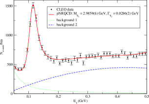
Figure 7: Fit of $d(\Gamma_{\rm mag}+\Gamma_{\rm ele})/dE_{\gamma}$ plus background [33] on the CLEO data of [34].

Fitting (9) plus (11) plus background on the CLEO data of [34], we get Fig. 7 [33]. The line-shape parameters are

(13) $$M_{\eta_{c}}=2985.9\pm 0.6\,\hbox{(fit)}\,\hbox{MeV}\,,\qquad\qquad\Gamma_{\eta_{c}}=28.6\pm 0.2\,\hbox{(fit)}\,\hbox{MeV}\,,$$

where theoretical errors have not been included. Besides $M_{\eta_{c}}$ and $\Gamma_{\eta_{c}}$ the fitting parameters are the overall normalization, the signal normalization, and (three) background parameters.

A study of electric transition in quarkonium in pNRQCD has been presented in [35].

5 $\Upsilon(1S)$ thermal width for $T{\ \lower-1.2pt\vbox{\hbox{\hbox to0.0pt{$<$\hss}\lower 6.0pt\vbox{\hbox{$\sim$}}}}\ }2T_{c}$

The bottomonium vector ground state, $\Upsilon(1S)$, produced in heavy-ion collisions at the LHC may possibly realize the hierarchy [36] (see also [37])

$$M_{b}\approx 5\;\hbox{GeV}\;>M_{b}\alpha_{\rm s}\approx 1.5\;\hbox{GeV}\;>\pi T\approx 1\;\hbox{GeV}\;>M_{b}\alpha_{\rm s}^{2}\approx 0.5\;\hbox{GeV}\;{\ \lower-1.2pt\vbox{\hbox{\hbox to0.0pt{$>$\hss}\lower 6.0pt\vbox{\hbox{$\sim$}}}}\ }m_{D},\Lambda_{\rm QCD}\,,$$

where $T$ is the temperature of the QCD plasma created by the collisions. A temperature $T$, such that $\pi T$ is of the order of 1 GeV, is about twice the critical temperature of the quark-gluon plasma formation, $T_{c}$; $m_{D}$ stands for the next-relevant thermal scale: the Debye mass. Studies of the $\Upsilon(1S)$ properties and, in particular, of its width in the above conditions are very timely because signals of bottomonium dissociation have just been seen by the CMS experiment [38].

According to the above hierarchy, the bound state is weakly coupled, the temperature is lower than $M_{b}\alpha_{\rm s}$, implying that the bound state is mainly Coulombic, and the effects due to the scale $\Lambda_{\rm QCD}$ and to the other thermodynamical scales may be neglected.

Figure 8: Leading thermal contribution to the singlet propagator from the scale $T$.

Integrating out $T$ from pNRQCD modifies pNRQCD into pNRQCD_HTL (see Fig. 1), whose Yang–Mills Lagrangian gets an additional hard thermal loop (HTL) part [39] and potentials get additional thermal corrections. One effect of the HTL part is to give a mass, $m_{D}$, to the temporal gluons. The leading thermal contribution to the potential is encoded in the diagram of Fig. 8, where thermal gluons couple to the singlet through chromoelectric dipole vertices (the difference with the diagram in Fig. 3 is in the gluon propagator). The loop momentum region is taken to be $k_{0}\sim T$ and $k\sim T$.

Figure 9: Gluon self-energy correction to the diagram of Fig. 8.

The gluon self-energy correction to the diagram in Fig. 8 is shown in Fig. 9. This diagram has an imaginary part that contributes to the thermal width of the state:

(14) $$\Gamma_{1S}^{(T)} = \left[-{{4\over 3}}\alpha_{\rm s}Tm_{D}^{2}\left(-{{2\over\epsilon}}+\gamma_{E}+\ln\pi-\ln{{T^{2}\over\mu^{2}}}+{{2\over 3}}-4\ln 2-2{{\zeta^{\prime}(2)\over\zeta(2)}}\right)\right.$$

$$\left.\hskip 207.7052pt-{{32\pi\over 3}}\,\alpha_{\rm s}^{2}\,T^{3}\,\ln 2\right]a_{0}^{2}\,,$$

where $\displaystyle a_{0}={{3\over 2M_{b}\alpha_{\rm s}}}$. The width is infrared (IR) divergent; the divergence has been regularized in dimensional regularization ($D=4+\epsilon$).

Figure 10: Landau-damping scatterings.

The origin of this thermal width may be traced back to the Landau-damping phenomenon, i.e. the scattering of heavy quarks with hard space-like particles in the medium (see Fig. 10). The Landau-damping phenomenon plays a crucial role in quarkonium dissociation [40]. It is when ${\rm Im}\leavevmode\nobreak\ V_{s}(r)|_{\rm Landau-damping}\sim{\rm Re}\leavevmode\nobreak\ V_{s}(r)\sim\alpha_{\rm s}/r$ that the quarkonium dissociates. The dissociation temperature is parametrically given by $\pi T_{\rm dissociation}\sim M_{b}g^{4/3}$. Note that the interaction is screened when $1/r\sim m_{D}$ and that in the weak coupling ($m_{D}\sim gT$) $\pi T_{\rm screening}\sim M_{b}g\gg\pi T_{\rm dissociation}$. The typical dissociation temperature, $T_{\rm dissociation}$, for the $\Upsilon(1S)$ is about 450 MeV [9], which implies that a temperature, $T$, such that $\pi T$ is about 1 GeV, is below the dissociation temperature.

Figure 11: Leading thermal contribution to the singlet propagator from the scale $E$. Gluons are HTL gluons.

Integrating out the energy scale $E$ from pNRQCD_HTL provides corrections to the mass and width of the quarkonium in the thermal bath. The leading diagram is shown in Fig. 11, where HTL gluons couple to the singlet through chromoelectric dipole vertices. The loop momentum region is taken to be $k_{0}\sim E$ and $k\sim E$. For $E\gg m_{D},\Lambda_{\rm QCD}$, the contribution to the thermal width of the $\Upsilon(1S)$ is given by

(15) $$\Gamma_{1S}^{(E)} = 4\alpha_{\rm s}^{3}T-{{64\over 9M_{b}}}\alpha_{\rm s}TE_{1}+{{32\over 3}}\alpha_{\rm s}^{2}T{{1\over M_{b}a_{0}}}+{{7225\over 162}}E_{1}\alpha_{\rm s}^{3}$$

$$-{{4\alpha_{\rm s}Tm_{D}^{2}\over 3}}\left({{2\over\epsilon}}+\ln{{E_{1}^{2}\over\mu^{2}}}+\gamma_{E}-{{11\over 3}}-\ln\pi+\ln 4\right)a_{0}^{2}+{{128\alpha_{\rm s}Tm_{D}^{2}\over 81}}{{\alpha_{\rm s}^{2}\over E_{1}^{2}}}\,I_{1,0}\,,$$

where $\displaystyle E_{1}=-{{4M_{b}\alpha_{\rm s}^{2}\over 9}}$ and $I_{1,0}=-0.49673$ (similar to the Bethe logarithm). The width is ultraviolet (UV) divergent. Note that the UV divergence of (15) cancels against the IR divergence of (14).

Figure 12: Singlet-to-octet break up diagram.

The thermal width $\Gamma_{1S}^{(E)}$, which is of order $\alpha_{\rm s}^{3}T$, is generated by the break up of a quark-antiquark colour-singlet state into an unbound quark-antiquark colour-octet state (see e.g. Fig. 12): a process that is kinematically allowed only in a medium. The singlet to octet break up is, therefore, a different phenomenon with respect to the Landau damping. In the situation $M_{b}\alpha_{\rm s}^{2}\gg m_{D}$, the first dominates over the second by a factor $(M_{b}\alpha_{\rm s}^{2}/m_{D})^{2}$ [5].

The complete thermal width up to ${\cal O}(m\alpha_{\rm s}^{5})$ is [8]:

(16) $$\Gamma_{1S}^{(\mathrm{thermal})} = \Gamma_{1S}^{(T)}+\Gamma_{1S}^{(E)}={{1156\over 81}}\alpha_{\rm s}^{3}T+{{7225\over 162}}E_{1}\alpha_{\rm s}^{3}+{{32\over 9}}\alpha_{\rm s}\,Tm_{D}^{2}\,a_{0}^{2}\,I_{1,0}$$

$$-\left[{{4\over 3}}\alpha_{\rm s}Tm_{D}^{2}\left(\ln{{E_{1}^{2}\over T^{2}}}+2\gamma_{E}-3-\ln 4-2{{\zeta^{\prime}(2)\over\zeta(2)}}\right)+{{32\pi\over 3}}\,\alpha_{\rm s}^{2}\,T^{3}\,\ln 2\right]a_{0}^{2}\,.$$

The width is an observable, therefore, finite and scheme independent. The logarithm, $\ln E_{1}^{2}/T^{2}$, is a relic of the cancellation between the IR divergence at the scale $T$ and the UV divergence at the scale $E$.

6 Conclusions

Our understanding of the theory of quarkonium has dramatically improved over the last fifteen years. An unified picture has emerged that is able to describe large classes of observables for quarkonium in the vacuum and in a medium. For the ground state, precision physics is possible and lattice data provide often a crucial complement. In the case of quarkonium in a hot medium, systematic treatments have disclosed new phenomena that may eventually be responsible for the quarkonium suppression observed in heavy-ion collisions.

Acknowledgements
I acknowledge financial support from the DFG cluster of excellence “Origin and structure of the universe” (www.universe-cluster.de) and from the DFG project BR4058/1-1 “Effective field theories for strong interactions with heavy quarks”.

References

• [1] N. Brambilla et al., Heavy quarkonium physics, CERN-2005-005, (CERN, Geneva, 2005) [arXiv:hep-ph/0412158].
• [2] N. Brambilla, A. Pineda, J. Soto and A. Vairo, Rev. Mod. Phys.  77, 1423 (2005) [arXiv:hep-ph/0410047].
• [3] T. Matsui and H. Satz, Phys. Lett.  B 178, 416 (1986).
• [4] Talk by M. Laine at this conference, arXiv:1108.5965 [hep-ph].
• [5] N. Brambilla, J. Ghiglieri, A. Vairo and P. Petreczky, Phys. Rev.  D 78, 014017 (2008) [arXiv:0804.0993 [hep-ph]].
• [6] M. A. Escobedo and J. Soto, Phys. Rev.  A 78, 032520 (2008) [arXiv:0804.0691 [hep-ph]].
• [7] A. Vairo, PoS CONFINEMENT8, 002 (2008) [arXiv:0901.3495 [hep-ph]].
• [8] N. Brambilla, M. A. Escobedo, J. Ghiglieri, J. Soto and A. Vairo, JHEP 1009, 038 (2010) [arXiv:1007.4156 [hep-ph]].
• [9] M. A. Escobedo and J. Soto, Phys. Rev.  A 82, 042506 (2010) [arXiv:1008.0254 [hep-ph]].
• [10] W. E. Caswell and G. P. Lepage, Phys. Lett. B 167, 437 (1986).
• [11] G. T. Bodwin, E. Braaten and G. P. Lepage, Phys. Rev. D 51, 1125 (1995) [Erratum-ibid. D 55, 5853 (1997)].
• [12] Talk by M. Butenschön at this conference, arXiv:1109.1740 [hep-ph].
• [13] A. Pineda and J. Soto, Nucl. Phys. Proc. Suppl.  64, 428 (1998) [arXiv:hep-ph/9707481].
• [14] N. Brambilla, A. Pineda, J. Soto and A. Vairo, Nucl. Phys.  B 566, 275 (2000) [arXiv:hep-ph/9907240].
• [15] N. Brambilla et al., Eur. Phys. J.  C 71, 1534 (2011) [arXiv:1010.5827 [hep-ph]].
• [16] L. Susskind, In Les Houches 1976, Proceedings, Weak and Electromagnetic Interactions At High Energies, 207-308 (Amsterdam, 1977).
• [17] Y. Schröder, Phys. Lett.  B 447, 321 (1999) [arXiv:hep-ph/9812205].
• [18] N. Brambilla, A. Pineda, J. Soto and A. Vairo, Phys. Rev.  D 60, 091502 (1999).
• [19] C. Anzai, Y. Kiyo and Y. Sumino, Phys. Rev. Lett.  104, 112003 (2010).
• [20] A. V. Smirnov, V. A. Smirnov and M. Steinhauser, Phys. Rev. Lett.  104, 112002 (2010).
• [21] B. A. Kniehl, A. A. Penin, Y. Schröder, V. A. Smirnov and M. Steinhauser, Phys. Lett.  B 607, 96 (2005) [arXiv:hep-ph/0412083].
• [22] N. Brambilla, J. Ghiglieri, P. Petreczky, A. Vairo, Phys. Rev.  D82, 074019 (2010). [arXiv:1007.5172 [hep-ph]].
• [23] N. Brambilla, X. Garcia i Tormo, J. Soto and A. Vairo, Phys. Lett.  B 647, 185 (2007).
• [24] M. Eidemüller and M. Jamin, Phys. Lett.  B 416, 415 (1998) [arXiv:hep-ph/9709419].
• [25] W. Fischler, Nucl. Phys. B 129, 157 (1977).
• [26] A. Billoire, Phys. Lett. B 92, 343 (1980).
• [27] A. Pineda and J. Soto, Phys. Lett.  B 495, 323 (2000).
• [28] N. Brambilla, X. Garcia i Tormo, J. Soto and A. Vairo, Phys. Rev.  D 80, 034016 (2009) [arXiv:0906.1390 [hep-ph]].
• [29] N. Brambilla, X. Garcia i Tormo, J. Soto and A. Vairo, Phys. Rev. Lett.  105, 212001 (2010) [arXiv:1006.2066 [hep-ph]].
• [30] S. Necco and R. Sommer, Nucl. Phys.  B 622, 328 (2002).
• [31] N. Brambilla, Y. Jia and A. Vairo, Phys. Rev.  D 73, 054005 (2006) [arXiv:hep-ph/0512369].
• [32] M. B. Voloshin, Mod. Phys. Lett.  A 19, 181 (2004).
• [33] N. Brambilla, P. Roig and A. Vairo, AIP Conf. Proc.  1343, 418 (2011) [arXiv:1012.0773 [hep-ph]]; TUM-EFT 26/11, in preparation.
• [34] R. E. Mitchell et al. [CLEO Collaboration], Phys. Rev. Lett.  102, 011801 (2009) [Erratum-ibid.  106, 159903 (2011)] [arXiv:0805.0252 [hep-ex]].
• [35] Talk by P. Pietrulewicz at this conference, TUM-EFT 24/11; N. Brambilla, P. Pietrulewicz and A. Vairo, TUM-EFT 25/11, in preparation.
• [36] A. Vairo, AIP Conf. Proc.  1317, 241 (2011) [arXiv:1009.6137 [hep-ph]].
• [37] Talk by J. Ghiglieri at this conference, arXiv:1108.5875 [hep-ph].
• [38] C. Silvestre for the CMS collaboration, arXiv:1108.5077 [hep-ex].
• [39] E. Braaten and R. D. Pisarski, Phys. Rev.  D 45, 1827 (1992).
• [40] M. Laine, O. Philipsen, P. Romatschke and M. Tassler, JHEP 0703, 054 (2007) [arXiv:hep-ph/0611300].