Multi-Hypothesis CRF-Segmentation of Neural Tissue in anisotropic EM volumes

Abstract

We present an approach for the joint segmentation and grouping of similar components in anisotropic 3D image data and use it to segment neural tissue in serial sections electron microscopy (EM) images. We first construct a nested set of neuron segmentation hypotheses for each slice. A conditional random field (CRF) then allows us to evaluate both the compatibility of a specific segmentation and a specific inter-slice assignment of neuron candidates with the underlying observations. The model is solved optimally for an entire image stack simultaneously using integer linear programming (ILP), which yields the maximum a posteriori solution in amortized linear time in the number of slices. We evaluate the performance of our approach on an annotated sample of the Drosophila larva neuropil and show that the consideration of different segmentation hypotheses in each slice leads to a significant improvement in the segmentation and assignment accuracy.

1 Introduction

Electron microscopy (EM) remains the only imaging technique with sufficient resolution for the elucidation of synaptic contacts between neurons [Briggman2006]. The acquisition of large volumes of brain circuitry is now possible with recent advances in automated imaging for EM. The next bottleneck in the reconstruction of neural circuits is the accurate reconstruction of 3D neural arbors from stacks of EM images [Jain2010]. Despite several efforts at automating the analysis of these highly stereotyped images, further improvements in overall accuracy are needed before automated methods can eliminate the tedious work currently needed to annotate large EM image datasets.

Current attempts at automatic labelling of anisotropic neural tissue in 3D-imaged serial sections can broadly be divided in two categories. (i) Binary segmentation based approaches try to identify the outlines of neurons within single slices [Jurrus2010, Kaynig2010, Kaynig2010a], and the results are used to establish geometrically consistent assignments of connected components that belong to one neuron. These approaches suffer from a high sensitivity to small errors: a missing piece of membrane alters the topological properties of the result. (ii) Over-segmentation based approaches merge small image regions within and between slices [Vazquez-Reina2010, Vitaladevuni2010]. The resulting optimization problem is solved approximately.

Our approach belongs to the first category. The improvements over current work are: (i) Our framework allows for rivaling concurrent segmentation hypotheses. This reduces the likelihood of missing crucial parts of the segmentation. (ii) All possible continuations of neural processes across slices are considered jointly with the segmentation hypotheses. Thus, higher-order relations between slices influence the segmentation. (iii) A globally consistent and optimal solution is found in amortized linear time in the number of slices. This is a prerequisite for the processing of large volumes.

An overview of our approach can be seen in Fig. 1. From the original images, per-pixel local features are extracted. Using several segmentations based on predictions of a pre-trained random forest classifier on the local features, segmentation hypotheses are extracted for each slice. These hypotheses are connected components of pixels (see Sec. 2). Given the hypotheses, two tasks have to be performed. Firstly, a subset of non-overlapping components has to be found to make up the segmentation of each slice. Secondly, assignments have to be established between the selected components of two subsequent slices. These assignments identify components that belong to the same neuron. We show how both tasks can be solved jointly by the introduction of binary assignment variables (see Sec. 3). A consistent and optimal segmentation and assignment can be found by MAP-inference in a conditional random field (CRF). Results presented in Sec. 4 show that our approach leads to a significant improvement in the segmentation and assignment accuracy.

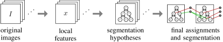
Figure 1: The proposed processing pipeline.

2 Generating Segmentation Hypotheses

To extract segmentation hypotheses for each slice, we use a parameterized model to solve a binary image segmentation task. Given a field of per-pixel local features $x$, the task is to maximize the conditional probability over a binary segmentation $y$:

$$p(y|x)=\frac{1}{Z(x)}\exp\left[\lambda_{D}\sum_{i\in\Omega}D(x_{i},y_{i})-\lambda_{S}\sum_{i,j\in\mathcal{N}}S(y_{i},y_{j},x)-\lambda_{N}\sum_{i\in\Omega}y_{i}\right]$$ (1)

Here, $\Omega\subset\mathbb{R}^{2}$ is the image domain and $D(x_{i},y_{i})=log\,p(x_{i}|y_{i})$ is the log-likelihood of pixel $i\in\Omega$ belonging to fore- or background, as given by a pre-trained random forest classifier. The set $\mathcal{N}\subset\Omega\times\Omega$ contains all pairs of 8-connected neighboring pixels. $Z(x)$ is the partition function. The second term in the exponent ensures smoothness of the segmentation, while favoring label changes in image regions of strong spatial gradients [Kohli2010]:

$$S_{ij}(y_{i},y_{j},x)=\frac{\exp\left[-\frac{g^{2}(x_{i},x_{j})}{2\sigma^{2}}\right]}{\lVert i-j\rVert}(1-\delta_{y_{i}=y_{j}})\text{.}$$ (2)

Here, $g(x_{i},x_{j})$ measures the difference in gray-levels, $\lVert.\rVert$ denotes the length of a vector, and $\delta$ is the Kronecker-delta. $\sigma$ is a parameter of the smoothness term.

The last term in the exponent of (1) is a prior on the expected number of pixels assigned to the label ‘neuron’. The scalars $\lambda_{D}$, $\lambda_{S}$, and $\lambda_{N}$ are parameters of the probability distribution. Since the exponent in (1) is submodular, the inference task can be seen as a parametric max-flow problem which can be solved efficiently [Boykov2004]. However, finding an optimal set of parameters is a non-trivial task and one cannot expect a fixed set of parameters to perform well on all images [Kolmogorov2007]. We go further and claim that a fixed set of parameters cannot even be expected to perform well on all areas of one image. Therefore, we enumerate several local segmentation hypotheses by variation of $\lambda_{N}$ (Fig. 2). This can be done efficiently by several warm-started graph-cuts [Kohli2010], from which we obtain a series of segmentations. Each segmentation consists of a set of connected components ${\boldsymbol{C}}^{i}\subset\Omega$ that are labelled as neurons. Each of these components is considered as one segmentation hypothesis. As $\lambda_{N}$ decreases, these components can grow and merge, thus establishing a tree-shaped subset hierarchy, the so-called component tree [Jones1997] (Fig. 3). All components which do not meet a criterion for stability over the range of values of $\lambda_{N}$ are removed [Matas2004]. Let $\mathcal{C}^{z}$ denote the set of all remaining components of slice $z$. Any consistent subset $\mathcal{S}^{z}\subset\mathcal{C}^{z}$ of these hypotheses yields a valid segmentation of this slice. A subset is consistent if none of the containing components overlap, i.e., ${\boldsymbol{C}}^{i}\cap{\boldsymbol{C}}^{j}=\varnothing$ for all ${\boldsymbol{C}}^{i},{\boldsymbol{C}}^{j}\in\mathcal{S}^{z}$ with $i\neq j$. In the following, we show how we find the optimal consistent segmentation by considering the assignments of hypotheses between pairs of adjacent slices.

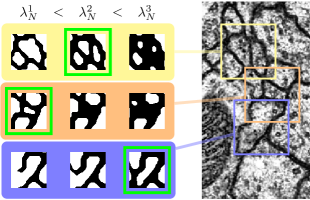
Figure 2: Segmentation results of nearby image regions for different values of $\lambda_{N}$. This parameter determines how many of the pixels are getting assigned to neurons. The desired segmentation result for each case is highlighted in green.

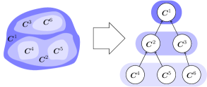
Figure 3: Visualisation of the segmentation hypotheses extraction. For different values of the prior parameter $\lambda_{N}$ (shades of blue) connected components of the segmentation are found (left side). The subset relation of these connected components define the component tree (right side).

3 Assignment Model

For each possible assignment of a segmentation hypothesis in one slice to a hypothesis in the previous or next slice, we introduce one binary assignment variable. This variable is set to $1$ if the involved hypotheses and their mutual assignment are accepted.

Let $m$ be the number of all possible assignments. A binary vector ${\boldsymbol{a}}\in\{0,1\}^{m}$ of assignment variables is created similarly to the method proposed in [Padfield2010]. Each possible continuation of a hypothesis ${\boldsymbol{C}}^{i}$ in slice $z$ to a hypothesis ${\boldsymbol{C}}^{j}$ in slice $z+1$ is represented by a variable $a^{i\rightarrow j}$. A split of ${\boldsymbol{C}}^{i}$ in slice $z$ to ${\boldsymbol{C}}^{j}$ and ${\boldsymbol{C}}^{k}$ in slice $z+1$ is represented as $a^{i\rightarrow j,k}$. Similarly, each possible merge is encoded as $a^{i,j\rightarrow k}$. Appearances and disappearances of neurons are encoded as assignments to a special end node ${\boldsymbol{E}}$, i.e., for each hypothesis ${\boldsymbol{C}}^{i}$ we introduce two variables $a^{i\rightarrow{\boldsymbol{E}}}$ and $a^{{\boldsymbol{E}}\rightarrow i}$. For the possible assignments, only components within a threshold distance to each other are considered. Thus, the number of assignment variables is linear in the number of segmentation hypotheses. See Fig. 4 for examples of assignments of a single segmentation hypothesis. We find the optimal segmentation and assignment via MAP-inference on the following CRF:

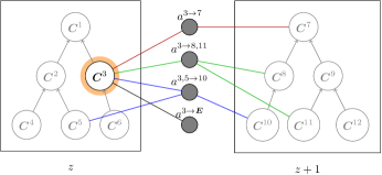
Figure 4: Examples of the four outgoing assignment categories for a single segmentation hypothesis (orange): A continuation (red) is modelled for each hypothesis in the next slice that is within a threshold distance. Possible splits (green) and merges (blue) are enumerated for neighboring hypotheses in the respective slices. Again, the possible sources or targets of splits and merges are segmentation hypotheses within a threshold distance. The disappearance of a neuron is represented by a single assignment for each candidate (black).

$$p({\boldsymbol{a}}|\mathcal{C})=\frac{1}{Z(\mathcal{C})}\exp\left[-{\boldsymbol{c}}^{\sf T}{\boldsymbol{a}}-\sum_{{\boldsymbol{P}}\in\mathcal{P}}H({\boldsymbol{P}})-\sum_{1\leq i\leq n}E({\boldsymbol{a}}^{\rightarrow i},{\boldsymbol{a}}^{i\rightarrow})\right]\text{.}$$ (3)

Here, $\mathcal{P}$ denotes the set of all complete paths of the hypotheses trees. The set of all incoming and outgoing assignment variables for a hypothesis ${\boldsymbol{C}}^{i}$ is denoted by ${\boldsymbol{a}}^{\rightarrow i}$ and ${\boldsymbol{a}}^{i\rightarrow}$, respectively. Incoming assignment variables of a hypothesis ${\boldsymbol{C}}^{i}$ are all components of ${\boldsymbol{a}}$ that have ${\boldsymbol{C}}^{i}$ on the right side of the superscript. Outgoing assignment variables are defined analogously.

The first term in the exponent accounts for unary potentials determining the costs for each assignment. For that, a vector ${\boldsymbol{c}}\in\mathbb{R}^{m}$ is constructed, which is congruent to ${\boldsymbol{a}}$. The costs for one-to-one assignments are modelled as:

$$c^{i\rightarrow j}=\theta_{L}L({\boldsymbol{C}}^{ij})+\theta_{P}\lVert\overline{{\boldsymbol{C}}^{i}}-\overline{{\boldsymbol{C}}^{j}}\rVert^{2}+\theta_{S}\lvert{\boldsymbol{C}}^{i}\ominus{\boldsymbol{C}}^{j}\rvert^{2}\text{.}$$ (4)

Here, we write ${\boldsymbol{C}}^{ij}$ as a shorthand for ${\boldsymbol{C}}^{i}\cup{\boldsymbol{C}}^{j}$. The expression $\overline{{\boldsymbol{C}}^{i}}$ denotes the mean pixel position of the candidate ${\boldsymbol{C}}^{i}$; ${\boldsymbol{C}}^{i}\ominus{\boldsymbol{C}}^{j}$ is the mean-corrected symmetric set difference of candidates ${\boldsymbol{C}}^{i}$ and ${\boldsymbol{C}}^{j}$; $\lVert.\rVert$ denotes the Euclidean distance; and $\lvert.\rvert$ the cardinality of a set. The term $L({\boldsymbol{C}})$ is proportional to the probability of assigning all pixels of ${\boldsymbol{C}}$ to a neuron, i.e.,

$$L({\boldsymbol{C}})=\sum_{j\in{\boldsymbol{C}}}\left(D(x_{j},0)-D(x_{j},1)\right)\;+\sum_{j,k\in\mathcal{N};\atop j\in{\boldsymbol{C}},\;k\notin{\boldsymbol{C}}}S_{j,k}(y_{j},y_{k},x)\text{.}$$ (5)

In a similar way, we define the costs for splits:

$$c^{i\rightarrow j,k} =\theta_{L}L({\boldsymbol{C}}^{ijk})+\theta_{BP}\lVert\overline{{\boldsymbol{C}}^{i}}-\overline{{\boldsymbol{C}}^{jk}}\rVert^{2}+\theta_{BS}\lvert{\boldsymbol{C}}^{i}\ominus{\boldsymbol{C}}^{jk}\rvert^{2}$$

The merge cases are defined analogously. Costs for the appearance or disappearance of a neuron depend on the data term and the size of the component:

$$c^{i\rightarrow{\boldsymbol{E}}}=c^{{\boldsymbol{E}}\rightarrow i}=\theta_{L}L({\boldsymbol{C}}^{i})+\theta_{E}\lvert{\boldsymbol{C}}^{i}\rvert^{2}$$

The scalars $\theta_{L}$, $\theta_{P}$, $\theta_{S}$, $\theta_{BP}$, $\theta_{BS}$, and $\theta_{E}$ are parameters of the model.

The second and third terms in (3) are higher-order potentials that ensure the consistency of the solution. $H({\boldsymbol{P}})$ ensures that at most one of all incoming assignments of competing segmentation hypotheses is selected. Competing hypotheses are components that share some pixels, i.e., all components along one path in the hypotheses tree (see Fig. 5(a)). This hypothesis constraint ensures that each pixel is explained by at most one hypothesis and that at most one of the possible assignments is selected for each hypothesis.

$$H({\boldsymbol{P}})=\left\{\begin{array}[]{ll}0&\text{if}\;\sum_{i\in{\boldsymbol{P}}}\sum_{a\in{\boldsymbol{a}}^{\rightarrow i}}a\leq 1\\ \infty&\text{else}\end{array}\right.$$ (8)

$E({\boldsymbol{a}}^{\rightarrow i},{\boldsymbol{a}}^{i\rightarrow})$ ensures that if an incoming assignment was selected for a segmentation hypothesis, an outgoing assignment is selected as well. This explanation constraint guarantees a consistent sequence of assignments (see Fig. 5(b)).

$$E({\boldsymbol{a}}^{\rightarrow i},{\boldsymbol{a}}^{i\rightarrow})=\left\{\begin{array}[]{ll}0&\text{if}\;\sum_{a\in{\boldsymbol{a}}^{\rightarrow i}}a=\sum_{a^{\prime}\in{\boldsymbol{a}}^{i\rightarrow}}a^{\prime}\\ \infty&\text{else}\end{array}\right.$$ (11)

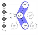
(a) hypothesis consistency

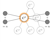
(b) explanation consistency

Figure 5: Visualization of the two types of consistency constraints. The hypothesis consistency 5(a) ensures that no pixel is assigned to more than one segmentation hypothesis: For each path of the component tree (blue), the sum of all incoming assignment variables (gray) has to at most one. The explanation consistency 5(b) ensures a continuous sequence of assignments: For each segmentation hypothesis (orange), the sum of all incoming assignment variables (from the previous image) has to be equal to the sum of all outgoing assignment variables (to the next image). The incoming or outgoing assignment variables for a component are all assignment variables that have the component as target or source, respectively.

Since the potentials $H$ and $E$ impose hard constraints and the remaining potentials are linear in ${\boldsymbol{a}}$, the MAP solution to (3) can be found by solving the following linear program.

(12)

Unfortunately, the constraint matrix of this linear program is not totally unimodular. Therefore, we have to enforce the integrality of the solution explicitly. The resulting optimization problem is an instance of an integer linear program (ILP), which we solve using the IBM CPLEX solver [cplex].

4 Results

We evaluated the performance of our approach on an annotated sample of Drosophila larva neural tissue [Cardona2010]. This publicly available data set consists of 30 serial sections (50 nm), imaged with transmission electron microscopy at a resolution of 4x4x50 nm/pixel. The image volume contains a 2x2x1.5 micron cube of neuropil tissue. The dataset includes labels of cellular membranes, cytoplasms and mitochondria of all 170 neural processes contained in the dataset.

To measure the accuracy of our method, we use the edit distance between the result and the ground-truth, i.e., the number of splits and merges a human operator would need to perform to restore the ground-truth [Vitaladevuni2010]. In contrast to the measure proposed in [Jain2010], we count every false merge, even if the same objects are involved. Each missed neuron segment in a slice is counted as one merge error and each falsely introduced neuron segment is counted as one split error. Between the slices, we count each missed assignment as a split error and each falsely introduced assignment as a merge error.

To evaluate the performance of our approach in comparison to approaches that do not allow local variations in the segmentation parameters (which is the case for all existing approaches that we know of), we carried out a series of experiments with fixed $\lambda_{N}$ (see Eq. 1). In particular, we took 34 equidistant samples of $\lambda_{N}$ in an interval reaching from obvious over- to under-segmentation of the images. Note that the clamping of the parameter $\lambda_{N}$ corresponds to not considering conflicting hypotheses: all the component trees have a depth of one. All other parameters of the pipeline do not change between the experiments, and have been found via a grid-search in the parameter space. We compare the results of this series with a single run of our proposed method that does allow for local variations of $\lambda_{N}$. In Fig. 6 we show the edit distance for each $\lambda_{n}$ in the series as well as for our approach normalized by the number of neurons in the dataset. Our data demonstrates that the single run with local variation of $\lambda_{N}$ is superior to all the cases in which $\lambda_{N}$ was fixed.

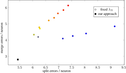
Figure 6: Comparison of the accuracy of our approach with different segmentation hypotheses (black square) against a series of experiments without segmentation hypotheses (colored circles). The consideration of different segmentations is superior to all possible single segmentations. The single segmentation experiments cover the whole range from under-segmentation (blue) to oversegmentation (red).

In Fig. 7 we show a representative segmentation example of five subsequent slices using our approach. In the same figure we give the inference time for the processing of the test dataset with different number of slices. The results indicate that the solution to the optimization task can be found in amortized linear time.

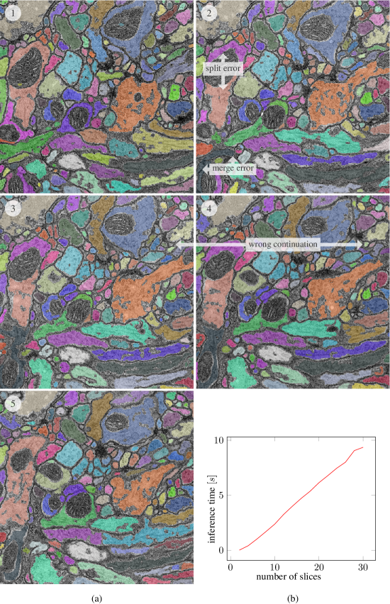
Figure 7: Sample of the segmentation result of five subsequent slices (a) and inference time (b). Examples of each error type are highlighted. Colors indicate the assignment of components between the slices.

5 Conclusion

We presented a novel approach for the joint segmentation and assignment of similar regions in anisotropic 3D image data with an amortized linear running time in the number of slices. On an annotated sample of neural tissue we could show that the consideration of different segmentation hypotheses significantly improves the accuracy of the segmentation and grouping of neural processes. The probabilistic formulation of our approach is particularly useful in semi-interactive environments, where human-reconstructed neurons can help resolving ambiguity. Every manually traced neural process can be used to impose strong priors on the assignment model by decreasing the costs for the respective assignments.

Currently, the assignment costs are computed from simple statistics of the involved segmentation hypotheses. Improvements might be obtained by using more sophisticated features [Kaynig2010]. This will be the focus of further research.

6 Acknowledgements

This work was funded by the Swiss National Science Foundation. Parts of this work have been completed in collaboration with the Heidelberg Collaboratory for Image Processing.