Density of states deduced from ESR measurements on low-dimensional nanostructures; benchmarks to identify the ESR signals of graphene and SWCNTs

Abstract

Electron spin resonance (ESR) spectroscopy is an important tool to characterize the ground state of conduction electrons and to measure their spin-relaxation times. Observing ESR of the itinerant electrons is thus of great importance in graphene and in single-wall carbon nanotubes (SWCNTs). Often, the identification of CESR signal is based on two facts: the apparent asymmetry of the ESR signal (known as a Dysonian lineshape) and on the temperature independence of the ESR signal intensity. We argue that these are insufficient as benchmarks and instead the ESR signal intensity (when calibrated against an intensity reference) yields an accurate characterization. We detail the method to obtain the density of states from an ESR signal, which can be compared with theoretical estimates. We demonstrate the success of the method for K doped graphite powder. We give a benchmark for the observation of ESR in graphene.

I Introduction

Electron spin resonance (ESR) has proven to be an important method in identifying the ground state of strongly correlated electron systems. ESR helped e.g. to identify the ordered spin-density wave ground state in the Bechgaard salts Torrance et al. (1982) and for carbonaceous materials, ESR was key to discover the AC₆₀ (A=K, Rb, Cs) fulleride polymer Chauvet et al. (1994).
A natural expectation is that ESR can be applied for single-wall carbon nanotubes (SWCNTs) Iijima and Ichihashi (1993) and graphene Novoselov et al. (2004), which are the two novel members of the carbon nanostructure family. The ESR literature on graphene is yet restricted to a single report Ćirić et al. (2009). Although there exists larger literature on the SWCNTs, the situation is yet unclear. In general, the ESR signal on itinerant electrons yields a direct measurement of the spin-relaxation time (often called as spin-decoherence time), $T_{1}$, through the relation: $T_{1}=1/\gamma\Delta B$, where $\Delta B$ is the homogeneous ESR line-width and $\gamma/2\pi=28.0\,\text{GHz/T}$ is the electron gyromagnetic ratio. $T_{1}$ is the central parameter which characterizes the usability of the materials for spintronics. This explains the motivation of the ESR studies on graphene and SWCNTs.
One important question is whether the ESR signal of the itinerant (i.e. the conduction electrons) can be observed at all. It was argued on a theoretical basis Dóra et al. (2008) that it cannot be observed due to the Tomonaga-Luttinger liquid ground state of the metallic SWCNTs Bockrath et al. (1999); Ishii et al. (2003); Rauf et al. (2004). It seemed that the only way to explore the local magnetism in SWCNTs is to spin label it either by means of ¹³C nuclei Singer et al. (2005) or by an electron spin label Simon et al. (2006). The literature situation on the SWCNT ESR studies is conflicting, and it is reviewed herein without any judgement on validity. Petit et al. Petit et al. (1997) reported the observation of the ESR signal of itinerant electrons. Salvetat et al. Salvetat et al. (2005) reported that the ESR signal occuring around $g\approx 2$ is caused by defects in the SWCNTs. Likodimos et al. Likodimos et al. (2007) reported that a similar signal is related to the itinerant electrons with a possible antiferromagnetic order at low temperature. Corzilius et al. Corzilius et al. (2008) reported the observation of the itinerant electron ESR in SWCNT samples prepared by chemical vapor deposition.

Often, the identification of the itinerant electron ESR signal is based on two facts: the asymmetry of the ESR lineshape (also known as a Dysonian) and the temperature independence of the ESR signal intensity. The Dysonian lineshape also occurs for localized spins (e.g. for paramagnetic impurities) which are embedded in a metal thus this property cannot be used for the above identification. This is discussed as Eq. 3.6 in the seminal paper of Feher and Kip as the ”slowly diffusing magnetic dipole case” Feher and Kip (1955). The temperature independence of the ESR intensity could be observed for localized paramagnetic spins when they are embedded in a metal with increasing conductivity, $\sigma$ with decreasing temperature; then the microwave penetration depth $\lambda=\sqrt{\frac{2}{\mu_{0}\omega\sigma}}$ (here $\mu_{0}$ is the permeability of the vacuum and $\omega$ is the frequency of the microwaves).

There has been remarkable progress in the quest for the intrinsic ESR signal in SWCNTs using samples made of nanotubes separated according to their metallicity Arnold et al. (2006). However, both kinds of samples, i.e. those made of purely metallic or semiconducting nanotubes shows similar ESR signals Havlicek et al. (2010), thus the situation remains unresolved.

A parallel situation happened for high $T_{c}$ superconductors: soon after their discovery Bednorz and Müller (1986) several reports claimed to have observed the ”intrinsic” ESR signal in these compounds. Later it turned out for all studies that the signal of parasitic phases (which happen to have strong paramagnetic signals), the so-called green and brown-phases were observed. Later, spin labeling (e.g. Gd substituting Y in YBa₂Cu₃O_7-δ) turned out to be successful to study the electronic structure Jánossy et al. (1994).

The ESR signal of itinerant electrons in the SWCNTs is expected to have i) a $g$-factor near 2, ii) a line-width, $\Delta B$ smaller than 1 mT, and iii) a signal intensity corresponding to the low density of states (DOS) with no temperature dependence. All properties present a significant hindrance for the signal identification since most impurity in carbon have $g\approx 2$, a maximum 1 mT line-width, and the Curie spin-susceptibility of even a small amount of impurity overwhelms the small Pauli susceptibility of the itinerant electrons. Since nothing is known about the $g$-factor and the line-width a priori, only the magnitude of the calibrated ESR signal when compared to the theoretical estimates of the Pauli spin-susceptibility provides a clear-cut ESR signal identification in graphene or SWCNTs.

Here, we outline the method to determine the calibrated ESR signal intensity and the resulting DOS in one- and two-dimensional carbon. The method is demonstrated for K doped graphite powder which is regarded as a model system of biased graphene Grueneis et al. (2009). A good agreement is obtained between the theoretical and expeirmental DOS for the KC₈ doped graphite system. We note, that a similar program was applied successfully when the ESR signals of Rb₃C₆₀ Jánossy et al. (1993) and MgB₂ Simon et al. (2001) were discovered. We give benchmarks which can be used to decide whether the ESR of the itinerant electrons is observed in graphene.

II Experimental

We used commercial graphite powder (Fischer Scientific) and potassium (99.95 % purity: Sigma-Aldrich) for the intercalation experiments. The graphite powder (3 mg) was mixed with 3 mg MnO:MgO powder (Mn concentration 1.5 ppm) and ground in a mortar. MgO separates the graphite powder pieces, which enables the penetration of exciting microwave and its Mn content acts as an ESR intensity standard. The mixture was vacuum annealed at 500 $\mathrm{{}^{\circ}C}$ for 1 h in an ESR quartz tube and inserted into an Ar glove-box without air exposure. Alkali doping was performed by heating the ESR quartz tube containing the graphite powder and potassium for 29 hours using the standard temperature gradient method in Ref. Dresselhaus and Dresselhaus (1981) to obtain Stage I, i.e. KC₈ intercalated graphite. ESR measurements were performed with a JEOL X-band spectrometer at room temperature.

III Results and discussion

Table 1: The Curie and the Pauli spin-susceptibilities in three and two dimensions. Note that in two dimensions $A_{c}$ replaces $V_{c}$ in the expressions.

	Curie susceptibility				Pauli susceptibility				Units
SI		Gaussian		SI		Gaussian		SI 3D (2D)		Gaussian 3D (2D)
$\displaystyle\mu_{0}\frac{g^{2}S(S+1)\mu_{\text{B}}^{2}}{\displaystyle 3k_{\text{B}}T}\frac{1}{V_{c}}$		$\displaystyle\frac{g^{2}S(S+1)\mu_{\text{B}}^{2}}{\displaystyle 3k_{\text{B}}T}\frac{1}{\displaystyle V_{c}}$		$\displaystyle\mu_{0}\frac{g^{2}\mu_{\text{B}}^{2}}{4}\varrho(\varepsilon_{\text{F}})\frac{1}{\displaystyle V_{c}}$		$\displaystyle\frac{g^{2}\mu_{\text{B}}^{2}}{4}\varrho(\varepsilon_{\text{F}})\frac{1}{\displaystyle V_{c}}$		1(m)		$\mathrm{\displaystyle\frac{emu}{\displaystyle cm^{3}\cdot Oe}}\left(\mathrm{\displaystyle\frac{emu}{\displaystyle cm^{2}\cdot Oe}}\right)$

First, we discuss spin-susceptibility, $\chi_{s}$, calculated from the ESR signal in different dimensions. ESR spectroscopy measures the net amount of magnetic moments, which is an extensive thermodynamic variable, i.e. proportional to the sample amount. The corresponding intensive variable, which characterizes the material is the spin-susceptibility, $\chi_{s}$ which reads as:

$$\begin{split}\chi_{s}=\mu_{0}\cdot\frac{\sum m}{B_{\text{res}}\cdot V_{D}}\hskip 42.67912pt\mathrm{(SI)}\\ \chi_{s}=\frac{\sum m}{B_{\text{res}}\cdot V_{D}}\hskip 42.67912pt\mathrm{(Gaussian)}\end{split}$$ (1)

where $m$ is the magnetic moment, $B_{res}$ is the magnetic field of the resonance, $V_{D}$ is the volume in $D$ dimension ($D=2;3$), and $\mu_{0}$ is the permeability of the vacuum. Clearly, the unit of $\chi_{s}$ depends on the dimension $D$.

$\chi_{s}$ is either due to the Curie spin-susceptibility for non-interacting spins or the Pauli spin-susceptibility for itinerant electrons in a metal. The relevant expressions are given in Table 1. Therein, $A_{c}$/$V_{c}$ denotes the unit area/volume, $g$ is the $g$-factor, $\mu_{\text{B}}$ is the Bohr moment and $k_{\text{B}}$ is the Boltzmann constant. $S$ is the spin state of the non-interacting spins and $\varrho(\varepsilon_{\text{F}})$ is the DOS at the Fermi level in units of $\text{states}/\text{eV}\cdot unit$. Here, $unit$ refers to the unit chosen, e.g. for C₆₀ fulleride salts, the unit could be 60 carbon atoms. Then the DOS is larger but so is the unit volume which cancels in the result. For graphene, the two atom basis is used as $unit$.

The ESR intensity of a metal can be calibrated against a Curie spin system with known amount of spins. This leads to the comparison of the Pauli and the Curie spin-susceptibilities:

$$\begin{split}\frac{I_{\text{ESR}}(\text{Pauli})}{I_{\text{ESR}}(\text{Curie})}=\frac{\sum m_{\displaystyle\text{Pauli}}}{\sum m_{\displaystyle\text{Curie}}}=\left(\frac{g_{\text{Pauli}}}{g_{\text{Curie}}}\right)^{2}\times\hskip 42.67912pt\\ \vskip 3.0pt plus 1.0pt minus 1.0pt\cr\frac{4}{3}S(S+1)\cdot k_{\text{B}}T\varrho(\varepsilon_{\text{F}})\frac{B_{\mathrm{res}}(\text{Pauli})}{B_{\mathrm{res}}(\text{Curie})}\cdot\!\frac{\left(\frac{\displaystyle V_{D}}{\displaystyle V_{c}(D)}\right)(\text{Pauli})}{\displaystyle\left(\frac{\displaystyle V_{D}}{\displaystyle V_{c}(D)}\right)(\text{Curie})}\end{split}$$ (2)

where $I_{\text{ESR}}$ denotes the ESR signal. $V_{D}$ and $V_{c}(D)$ are the volume of the sample and the unit cell in $D$ dimensions, respectively. Note that $V_{D}/V_{c}(D)(\text{Pauli})=N(\text{ Pauli})$ is the number of units in the metallic sample and $V_{D}/V_{c}(D)(\text{Curie})=N(\text{Curie})$ is the number of Curie spins. Eq. (2) is correct for both SI and Gaussian units and is independent of the choice of $unit$, as expected.

For $S=1/2$ and $g_{\text{Pauli}},g_{\text{Curie}}\approx 2$, Eq. (2) simplifies to:

$$\begin{split}\frac{I_{\text{ESR}}(\text{Pauli})}{I_{\text{ESR}}(\text{Curie})}=k_{\text{B}}T\varrho(\varepsilon_{\text{F}})\frac{N(\text{ Pauli})}{N(\text{ Curie})}.\end{split}$$ (3)

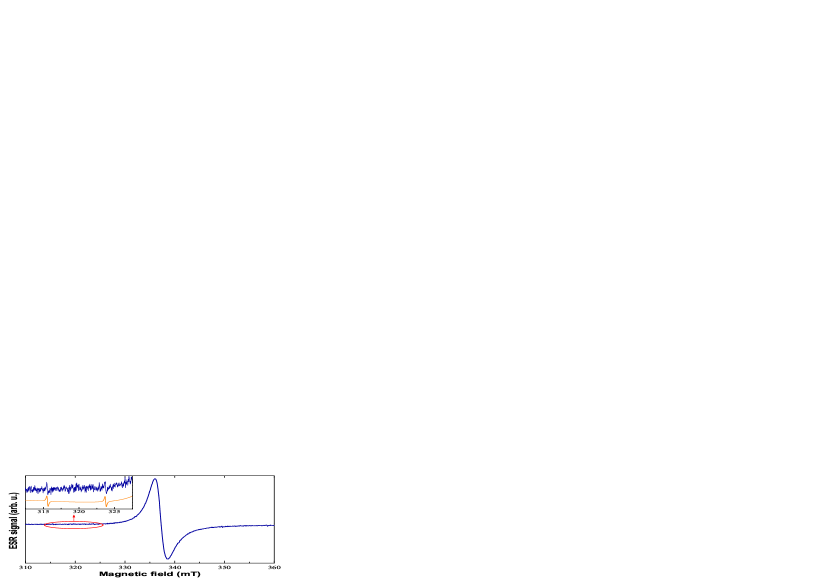
Figure 1: ESR spectrum of saturated K doped graphite powder sample at $T=$300 K. The inset shows a zoom on the ESR spectrum showing the presence of the six lines of the $\mathrm{Mn^{2+}}$ hyperfine structure. The solid curve is a fit.

Table 2: Parameters of the $\chi_{s}$ calibration of KC₈.

	Mn:MgO	Graphite
$\left\langle S\cdot(S+1)\right\rangle$	9/4
$M_{\mathrm{mol}}$ [g/mol]	40	12
$m$ [mg]	3	3
$C_{\mathrm{spin}}$	1.5 ppm	1
$I_{\mathrm{ESR}}$	$6\cdot 5.3\cdot 10^{-3}$	205

We present the case of KC₈ as an example of the ESR intensity calibration. In Fig. 1, we show the ESR signal of the mixture of MnO:MgO and saturated K doped graphite. Parameters of the calibration are given in Table 2: $C_{\mathrm{spin}}$ is the spin concentration and the effective $\left\langle S\cdot(S+1)\right\rangle_{\mathrm{Mn^{2+}}}=9/4$ as only the $-1/2\rightarrow 1/2$ transition is observed from the 5 Zeeman transitions of the Mn²⁺ ($S=5/2$) Abragam and Bleaney (1970).

The sample content gives: $N(\text{Pauli})/N(\text{Curie})\approx 3.33$ and Eq. (2) yields $\varrho(\varepsilon_{\text{F}})\approx 0.34(2)\;\mathrm{states/(eV\cdot C\>atom)}$, in good agreement with $\varrho(\varepsilon_{\text{F}})=0.327\;\mathrm{states/(eV\cdot C\>atom)}$ obtained by specific heat measurements Dresselhaus and Dresselhaus (1981).

In the following, we analyze the case of graphene. There, $A_{c}=5.24$ Å${}^{2}/(\text{unit cell})$ is the graphene elementary cell and the DOS, at $T=0$ and $\Gamma=0$ ($\Gamma$ is the damping parameter), reads as a function of the chemical potential $\mu$ Castro Neto et al. (2009):

$$\begin{split}\varrho(\mu)=\frac{2A_{c}\mu}{\pi\hbar^{2}v^{2}_{\text{F}}}.\end{split}$$ (4)

Here, $v_{\text{F}}\approx 10^{6}\,\text{m/s}$ is the Fermi velocity. Consequently, $\varrho(\mu)=\mu\cdot 0.0770\,\text{states/(eV}^{2}\cdot\text{unit cell})$ if $\mu$ is measured in eV. Thus Eq. (3) (in two dimensions) at room temperature reads:

$$\begin{split}\frac{\sum m_{\displaystyle\text{gr}}}{\sum m_{\displaystyle\text{Curie}}}=\underbrace{0.026\cdot 0.0770}_{\approx 1/500}\cdot\mu[\text{eV}]\frac{N(\text{gr})}{N(\text{Curie})}\end{split}$$ (5)

$N(\text{gr})$ is the number of graphene unit cells in the sample.

Finally, we assess the feasibility of ESR spectroscopy on graphene. ESR spectrometer performance is given by the limit-of-detection (LOD₀) i. e. the number of $S=1/2$ Curie magnetic moments at room temperature which are required for a signal-to-noise ratio of $S/N=10$ for $\Delta B=0.1$ mT linewidth, and 1 s/spectrum-point time constant. For modern spectrometers LOD${}_{0}=10^{10}$ spins/0.1 mT. To calculate the LOD for a broadened ESR line, LOD$(\Delta B)$, we introduce a function to track the effect of broadening:

$$\begin{split}f(\Delta B)=\left\{\begin{array}[]{lr}\frac{\displaystyle\Delta B}{\displaystyle 0.1\,\text{mT}}&\hskip 14.22636pt\text{if}\hskip 14.22636pt\Delta B\leq 1\,\text{mT}\\ \vskip 3.0pt plus 1.0pt minus 1.0pt\cr\frac{\displaystyle\Delta B^{2}}{\displaystyle 0.1\,\text{mT}^{2}}&\hskip 14.22636pt\text{if}\hskip 14.22636pt\Delta B>1\,\text{mT}\\ \end{array}\right.\end{split}$$ (6)

This function is 1 if $\Delta B=0.1\,\text{mT}$ and it is 10 if $\Delta B=1\,\text{mT}$ which is the usual maximum modulation amplitude. For line-widths above this value, the function grows quadratically, which describes that the amplitude of the derivative ESR signal drops quadratically. Using this function: LOD$(\Delta B)=$LOD${}_{0}\cdot f(\Delta B)$. Comparison with Eq. (5) yields that numerically ($\mu$ in eV units)

$$\begin{split}\text{LOD}(\text{gr})=500/\mu\cdot\text{LOD}_{0}\cdot f(\Delta B)\end{split}$$ (7)

is the LOD for graphene. We could conclude that

$$\begin{split}A_{\text{lb}}(\text{gr})=500/\mu\cdot\text{LOD}_{0}\cdot f(\Delta B)\cdot A_{c}\end{split}$$ (8)

which gives a lower bound for the area of the graphene sheet which enables the ESR measurement. Assuming a $\Delta B=0.1$ mT and a shift in chemical potential by gate bias of $\sim$0.2 eV we estimate $A_{\text{lb}}(\text{gr})\approx 1.3\,\mathrm{mm^{2}}$.

IV Summary

In summary, we detailed the method of obtaining the calibrated ESR intensity and the DOS in carbonaceous materials. We argue that a similar analysis is required for the identification of the ESR signal of itinerant electrons in SWCNT and graphene.

V Acknowledgements

Work supported by the OTKA Grant Nr. K 81492, and Nr. K72613, by the ERC Grant Nr. ERC-259374-Sylo, the Marie Curie ERG project CARBOTRON, and by the New Széchenyi Plan Nr. TÁMOP-4.2.1/B-09/1/KMR-2010-0002. BD acknowledges the Bolyai programme of the Hungarian Academy of Sciences. The Swiss NSF and its NCCR ”MaNEP” are acknowledged for support.

References

- Torrance et al. (1982) J. B. Torrance, H. Pedersen, and K. Bechgaard, Phys. Rev. Lett. 49, 881 (1982).
- Chauvet et al. (1994) O. Chauvet, G. Oszlányi, L. Forró, P. Stephens, M. Tegze, G. Faigel, and A. Jánossy, Phys. Rev. Lett. 72, 2721 (1994).
- Iijima and Ichihashi (1993) S. Iijima and T. Ichihashi, Nature 363, 603 (1993).
- Novoselov et al. (2004) K. S. Novoselov, A. K. Geim, S. V. Morozov, D. Jiang, Y. Zhang, S. V. Dubonos, I. V. Grigorieva, and A. A. Firsov, Science 306, 666 (2004).
- Ćirić et al. (2009) L. Ćirić, A. Sienkiewicz, B. Náfrádi, M. Mionić, A. Magrez, and L. Forró, Phys. Stat. Sol. B 246, 2558 (2009).
- Dóra et al. (2008) B. Dóra, M. Gulácsi, J. Koltai, V. Zólyomi, J. Kürti, and F. Simon, Phys. Rev. Lett. 101, 106408 (2008).
- Bockrath et al. (1999) M. Bockrath, D. H. Cobden, J. Lu, A. G. Rinzler, R. E. Smalley, L. Balents, and P. L. McEuen, Nature 397, 598 (1999).
- Ishii et al. (2003) H. Ishii, H. Kataura, H. Shiozawa, H. Yoshioka, H. Otsubo, Y. Takayama, T. Miyahara, S. Suzuki, Y. Achiba, M. Nakatake, T. Narimura, M. Higashiguchi, K. Shimada, H. Namatame, and M. Taniguchi, Nature 426, 540 (2003).
- Rauf et al. (2004) H. Rauf, T. Pichler, M. Knupfer, J. Fink, and H. Kataura, Phys. Rev. Lett. 93, 096805 (2004).
- Singer et al. (2005) P. M. Singer, P. Wzietek, H. Alloul, F. Simon, and H. Kuzmany, Phys. Rev. Lett. 95, 236403 (2005).
- Simon et al. (2006) F. Simon, H. Kuzmany, B. Náfrádi, T. Fehér, L. Forró, F. Fülöp, A. Jánossy, L. Korecz, A. Rockenbauer, F. Hauke, and A. Hirsch, Phys. Rev. Lett. 97, 136801 (2006).
- Petit et al. (1997) P. Petit, E. Jouguelet, J. E. Fischer, A. G. Rinzler, and R. E. Smalley, Phys. Rev. B 56, 9275 (1997).
- Salvetat et al. (2005) J.-P. Salvetat, T. Fehér, C. L’Huillier, F. Beuneu, and L. Forró, Phys. Rev. B 72, 075440 (2005).
- Likodimos et al. (2007) V. Likodimos, S. Glenis, N. Guskos, and C. L. Lin, Phys. Rev. B 76, 075420 (2007).
- Corzilius et al. (2008) B. Corzilius, K.-P. Dinse, K. Hata, M. Haluška, V. Skákalová, and S. Roth, Phys. Stat. Sol. B 245, 2251 (2008).
- Feher and Kip (1955) G. Feher and A. F. Kip, Physical Review 98, 337 (1955).
- Arnold et al. (2006) M. S. Arnold, A. A. Green, J. F. Hulvat, S. I. Stupp, and M. C. Hersam, Nature Nanotechn. 1, 60 (2006).
- Havlicek et al. (2010) M. Havlicek, W. Jantsch, M. Ruemmeli, R. Schoenfelder, K. Yanagi, Y. Miyata, H. Kataura, F. Simon, H. Peterlik, and H. Kuzmany, Phys. Stat. Sol. B 247 (2010).
- Bednorz and Müller (1986) J. G. Bednorz and K. A. Müller, Z. Phys. B 64, 189 (1986).
- Jánossy et al. (1994) A. Jánossy, J. R. Cooper, L.-C. Brunel, and A. Carrington, Physical Review B 50, 3442 (1994).
- Grueneis et al. (2009) A. Grueneis, C. Attaccalite, A. Rubio, D. V. Vyalikh, S. L. Molodtsov, J. Fink, R. Follath, W. Eberhardt, B. Buechner, and T. Pichler, Physical Review B 79, 205106 (2009).
- Jánossy et al. (1993) A. Jánossy, O. Chauvet, S. Pekker, J. R. Cooper, and L. Forró, Phys. Rev. Lett. 71, 1091 (1993).
- Simon et al. (2001) F. Simon, A. Jánossy, T. Fehér, F. Murányi, S. Garaj, L. Forró, C. Petrovic, S. L. Bud’ko, G. Lapertot, V. G. Kogan, and P. C. Canfield, Phys. Rev. Lett. 87 (2001), 10.1103/PhysRevLett.87.047002.
- Dresselhaus and Dresselhaus (1981) M. S. Dresselhaus and G. Dresselhaus, Advances in Physics 30, 132 (1981).
- Abragam and Bleaney (1970) A. Abragam and B. Bleaney, Electron paramagnetic resonance of transition ions (Oxford University Press, Oxford, England, 1970).
- Castro Neto et al. (2009) A. H. Castro Neto, F. Guinea, N. M. R. Peres, K. S. Novoselov, and A. K. Geim, Reviews of Modern Physics 81, 109 (2009).