Minimal seeds for shear flow turbulence: using nonlinear transient growth to touch the edge of chaos

Abstract

We propose a general strategy for determining the minimal finite amplitude disturbance to trigger transition to turbulence in shear flows. This involves constructing a variational problem that searches over all disturbances of fixed initial amplitude, which respect the boundary conditions, incompressibility and the Navier–Stokes equations, to maximise a chosen functional over an asymptotically long time period. The functional must be selected such that it identifies turbulent velocity fields by taking significantly enhanced values compared to those for laminar fields. We illustrate this approach using the ratio of the final to initial perturbation kinetic energies (energy growth) as the functional and the energy norm to measure amplitudes in the context of pipe flow. Our results indicate that the variational problem yields a smooth converged solution providing the amplitude is below the threshold amplitude for transition. This optimal is the nonlinear analogue of the well-studied (linear) transient growth optimal. At and above this threshold, the optimising search naturally seeks out disturbances that trigger turbulence by the end of the period, and convergence is then practically impossible. The first disturbance found to trigger turbulence as the amplitude is increased identifies the ‘minimal seed’ for the given geometry and forcing (Reynolds number). We conjecture that it may be possible to select a functional such that the converged optimal below threshold smoothly converges to the minimal seed at threshold. This seems at least approximately true for our choice of energy growth functional and the pipe flow geometry chosen here.

1 Introduction

Shear flows are ubiquitous in our everyday lives yet predicting their behaviour still remains an outstanding and important issue both scientifically and economically. Typically such flows become turbulent even though there may be an alternative linearly stable ‘basic state’, which is the simplest solution consistent with the driving forces and boundary conditions. This bistability means that the problem of transition comes down to understanding the laminar-turbulent boundary in phase space that divides initial conditions which lead to the turbulent state from those which relax back to the basic state. This boundary has more generally been labelled the ‘edge of chaos’, allowing for transient turbulence (Skufca et al. 2006). There have been notable recent successes in tracking parts of this boundary which, because it is a hypersurface in phase space, can be approached by a simple bisection technique (Itano & Toh 2001, Skufca, Yorke & Eckhardt 2006, Schneider, Eckhardt & Yorke 2007, Duguet, Willis & Kerswell 2008). As this technique is based upon integrating the governing Navier-Stokes equations forward in time, only the parts of the edge near (relative) attractors embedded in the edge are revealed by this tracking approach.

Interestingly, these attracting regions invariably seem to be on perturbation energy levels well above those known to be sufficient to trigger transition. Viswanath & Cvitanovic (2009) provide a good illustration of this in a short pipe of length $\pi$ diameters, which they numerically simulate with $85,715$ degrees of freedom. By only mixing three fixed flow fields, they identify initial conditions which experience an $O(10^{4})$ magnification of the (perturbation) energy in approaching a travelling wave thought to be embedded in the edge relative attractor (Schneider, Eckhardt & Yorke 2007, Pringle & Kerswell 2007): see their Table 4 for Reynolds number $Re=2000$. Duguet, Brandt and Larsson (2010) tackle the same question in plane Couette flow, finding evidence for energy growth on the edge of over $10^{2}$ at $Re=400$ for a pair of oblique waves (see their Figure 9 where the plateau edge energy is $O(5\times 10^{-3})$). Initial conditions with low energies on the edge represent energy-efficient targets to trigger transition, as an infinitesimal perturbation of these states will lead to transition. The most efficient of all perturbations will be the flow field having the lowest energy $E_{c}$ on the edge, hereafter called the minimal seed for transition, which represents the closest (in perturbation energy norm) point of approach of the edge to the basic state in phase space. This represents the most dangerous disturbance to the basic state and as a result is of fundamental interest either from the viewpoint of triggering transition efficiently or, oppositely, in designing flow control strategies.

Currently, there are no accepted strategies for identifying minimal seeds beyond the impractical ‘brute force’ approach of surveying all initial conditions. The purpose of this paper is to continue to develop a new strategy initiated in Pringle & Kerswell (2010), hereafter referred to as PK10, based upon identifying finite-amplitude disturbance fields which, as they evolve via the full Navier-Stokes equations, maximise a key functional over a period of time. This key functional is taken here to be the energy growth of the disturbance over the time period as suggested in PK10 and Cherubini et al. (2010) in the boundary layer context. The rationale behind this is the observation that the minimal seed must experience considerable energy growth as it evolves in time up to the attracting plateau on the edge. In the special case of a unique steady relative attractor on the edge the minimal seed will be the optimal solution $\mbox{\boldmath$u$}^{*}_{0}(\mbox{\boldmath$x$})$ to the following variational problem: which initial condition on the edge (label this set $\Sigma$) will experience, for asymptotically long times $T$, the largest energy growth defined as

$${\cal G}(T):=\max_{\mbox{\boldmath$u$}_{0}\in\Sigma}\frac{\int\mbox{\boldmath$u$}(\mbox{\boldmath$x$},T)^{2}\,dV}{\int\mbox{\boldmath$u$}(\mbox{\boldmath$x$},0)^{2}\,dV}$$ (1)

where $\mbox{\boldmath$u$}(\mbox{\boldmath$x$},t)$ is the flow at time $t$ evolved via the Navier-Stokes equations from the initial condition $\mbox{\boldmath$u$}(\mbox{\boldmath$x$},0)=\mbox{\boldmath$u$}_{0}(\mbox{\boldmath$x$})$ (incompressibility is tacitly assumed throughout) and $\mbox{\boldmath$u$}=(u,v,w)$ is the perturbation velocity field obtained by subtracting the laminar state from the total velocity field (invariably used hereafter). The problem with pursuing this criterion is not the fact that the relative edge attractor may have a fluctuating energy as these fluctuations are typically small compared to the total growth, but confining competitor fields to the hard-to-define edge set $\Sigma$. A more practical approach can be manufactured by turning the problem around to consider the largest energy growth $G$ over all initial (incompressible) conditions of a given perturbation energy $E_{0}$, that is

$$G(T;E_{0}):=\max_{\mbox{\boldmath$u$}_{0}:\int\mbox{\boldmath$u$}_{0}^{2}\,dV=2E_{0}}\frac{\int\mbox{\boldmath$u$}(\mbox{\boldmath$x$},T)^{2}\,dV}{\int\mbox{\boldmath$u$}(\mbox{\boldmath$x$},0)^{2}\,dV}.$$ (2)

At precisely $E_{0}=E_{c}$ where the edge touches the energy hypersurface at one velocity state, this optimisation problem considers the growth of this state (the minimal seed) against the energy growth of all the other initial conditions below the edge. Given that these latter initial conditions lead to flows that grow initially but ultimately relax back to the basic state, it is reasonable to hypothesize that the minimal seed remains the optimal initial condition for the revised variational problem. A priori, the minimal seed energy $E_{c}(Re;{\rm geometry})$ is unknown but a very interesting quantity in its own right, as its behaviour indicates how the basin of attraction of the basic state shrinks with increasing $Re$. Hence, the variational problem (2) must be solved as an increasing function of $E_{0}$ until $E_{c}$ is reached. Knowing when this has occurred motivates the following hypothesis.

Hypothesis: For asymptotically large $T$, the minimal seed will be given by the flow field of initial energy $E_{0}$ which experiences the largest energy growth such that for any initial energies exceeding this $E_{0}=E_{c}$, the energy growth problem (2) fails to have a smooth solution.

This is actually a very strong statement which really contains two separate but related conjectures, the first being a necessary condition for the second.

Conjecture 1: For $T$ sufficiently large, the initial energy value $E_{fail}$ at which the energy growth problem (2) first fails (as $E_{0}$ is increased) to have a smooth optimal solution will correspond exactly to $E_{c}$.

Conjecture 2: For $T$ sufficiently large, the optimal initial condition for maximal energy growth at $E_{0}=E_{c}-\epsilon^{2}$ converges to the minimal seed at $E_{c}$ as $\epsilon\rightarrow 0$.

The idea behind the first conjecture is that the optimisation algorithm (2), in exploring the $E_{0}$-hypersurface for the optimal solution, will detect any state on the energy hypersurface that leads to turbulence, given that this leads to the highest values of $G$. Once the algorithm is dealing with a turbulent endstate at time $T$, the extreme sensitivity of the final state energy at $T$ to changes in the initial condition, due to exponential divergence of adjacent states, will effectively mean non-smoothness and prevent convergence. Crucially, if true, this means that the failure of the algorithm solving (2) should identify $E_{c}$ regardless of whether the minimal seed is the optimal solution of (2) for $E_{0}=E_{c}$ or not. The key feature for Conjecture 1 to hold is not the precise form of the functional being maximised, but the fact that the functional attains higher values for initial conditions that go turbulent than those in the basin of attraction of the basic state (other plausible choices include the final dissipation rate, the total dissipation which has recently been explored with success by Monokrousos et al (2011) in the context of plane Couette flow, or more general Sobolev norms which emphasize strain rates). The second, stronger conjecture, however, proposes that the optimal initial condition converged at $E_{0}<E_{c}$ values, approaches the minimal seed as $E\rightarrow E_{c}$. This implies that the energy growth functional is then a special choice which picks out the minimal seed. We present evidence in this paper to support both these conjectures.

The variational problem (2) in the limit of infinitesimally small energy $E_{0}$ reduces to the well-known (linear) transient growth problem (Gustavsson 1991, Butler & Farrell 1992, Reddy & Henningson 1993, Trefethen et al. 1993, Schmid & Henningson 1994). In this case, the evolution of the initial condition $\mbox{\boldmath$u$}_{0}$ is determined by the linearised Navier-Stokes equations and there are various ways to proceed: e.g. for a matrix-based approach see Reddy & Henningson (1993) and for a time-stepping approach see, for example, Luchini (2000). The optimal that emerges typically shows energy growth factors $G$ that scale with $Re^{2}$ (when optimisation is also carried out over $T$) due to the nonnormality of the linearised evolution operator. It has been common practice to assume that this linear optimal (LOP) (for vanishing $E_{0}$) is a good approximation to the minimal seed, as the energy of the minimal seed is ‘small’ compared to that of the basic flow or target turbulent flow. It was shown in PK10, however, that the presence of nonlinearity in the variational problem is crucial in revealing new nonlinear optimals (NLOPs) that emerge ‘in between’ i.e. for $0\,<\,E_{0}\,<\,E_{c}$. The calculations of PK10 were directed more at demonstrating the feasibility of including nonlinearity in the transient growth calculation and showing the dramatic manner in which this alters the established linear result than identifying the minimal seed. In particular, $T=T_{lin}$ was taken where $T_{lin}$ is the optimal growth time for the linear optimal (LOP) and is not asymptotically large. Numerical limitations of the simulation code used in PK10 (written from scratch as part of the first author’s thesis) also meant that getting close to the edge proved difficult. In this paper, we revisit those calculations using a well-tested parallel code (described in Willis & Kerswell 2009) to probe the ‘gap’ between $E_{fail}$ and $E_{c}$ noticed there.

The plan of the paper is as follows. Section 2 formulates the variational problem (2) and describes briefly the iterative scheme used to solve it. Section 3 analyses for the first time the mechanism by which the nonlinear optimal (NLOP) which emerged in PK10 attains more growth than the linear optimal (LOP). The results of PK10 are then extended to higher energies in section 4 to re-examine the reported gap between $E_{fail}$ and $E_{c}$. In section 5, a larger domain is studied using a longer optimisation time to provide a first test of the conjectures discussed above. Our results are summarised and discussed in section 6 with a glossary of terms following at the end.

2 Formulation

The context for our exploration is the problem of constant mass-flux fluid flow through a cylindrical pipe. With length scales nondimensionalised by half the pipe diameter $\mbox{$\frac{1}{2}$}D$ and velocities by the mean axial velocity $U$, the laminar flow is given by

$$\mbox{\boldmath$u$}_{lam}={\cal U}(s)\hat{\mathbf{z}}=2(1-s^{2})\hat{\mathbf{z}}$$ (3)

using cylindrical coordinates $(s,\phi,z)$ aligned with the pipe axis. In keeping with the majority of published work, results are reported in time units of $D/U$. Energies are nondimensionalised by the energy of the laminar flow in the same domain. We then consider a perturbation to this laminar profile such that the full velocity field is given by

$${\cal U}(s)\hat{\mathbf{z}}+\mbox{\boldmath$u$}(s,\phi,z,t),$$ (4)

where $\mbox{\boldmath$u$}=(u,v,w)$ and for convenience define the volume integral

$$\langle\ldots\rangle=\int_{0}^{L}\int_{0}^{2\pi}\int_{0}^{1}\ldots s\mathrm{d}s\,\mathrm{d}\phi\,\mathrm{d}z.$$ (5)

In order to calculate the initial condition that produces the most energy growth, we use a variational approach pioneered for the linearised problem (Luchini & Bottaro 1998, Andersson, Berggren & Henningson 1999, Luchini 2000, Corbett & Bottaro 2000) but now recently extended to incorporate the full Navier-Stokes equations (PK10, Cherubini et al. 2010, Monokrousos et al. 2011: also see Zuccher et al. 2006 for earlier work using the boundary layer equations). The functional we choose is defined as

$$\mathscr{L}:=\langle\mbox{$\frac{1}{2}$}\mbox{\boldmath$u$}(\mbox{\boldmath$x$},T)^{2}\rangle - \lambda\bigg{[}\langle\mbox{$\frac{1}{2}$}\mbox{\boldmath$u$}(\mbox{\boldmath$x$},0)^{2}\rangle-E_{0}\bigg{]}$$ (6)

$$- \int_{0}^{T}\langle\boldsymbol{\nu}\cdot\bigg{[}\frac{\partial\mathbf{u}}{\partial t}+{\cal U}\frac{\partial\mathbf{u}}{\partial z}+{\cal U}^{\prime}u\mathbf{\hat{z}}-\mbox{\boldmath$u$}\times\nabla\times\mbox{\boldmath$u$}+\nabla p-\frac{1}{Re}\nabla^{2}\mathbf{u}\bigg{]}\rangle\mathrm{d}t$$

$$- \int_{0}^{T}\langle\Pi\nabla\cdot\mathbf{u}\rangle\mathrm{d}t-\int_{0}^{T}\Gamma(t)\langle\mathbf{u}\cdot\mathbf{\hat{z}}\rangle\mathrm{d}t.$$

This functional will be maximised by the same flow field as problem 2. It is equivalent to finding the flow field with greatest energy at time $t=T$, subject to four conditions applied through Lagrange multipliers - namely that the initial condition, $\mbox{\boldmath$u$}(\mbox{\boldmath$x$},0)$ has kinetic energy $E_{0}$ and that it evolves subject to the incompressible Navier-Stokes equations with fixed mass flux along the pipe. The last constraint introduces a slight subtlety in that the pressure field must be subdivided into a time-dependent constant pressure gradient part $\Lambda(t)z$ which adjusts to maintain constant mass flux and a strictly (spatially-) periodic part $\hat{p}$ so that

$$p:=\Lambda(t)z+\hat{p}(s,\phi,z,t).$$ (7)

The Lagrange multipliers $\boldsymbol{\nu}=(\nu_{s},\nu_{\phi},\nu_{z})$, $\Pi$ and $\Gamma$ are known as the adjoint variables. The function $\mathscr{L}$ will be maximised when all of its variational derivatives are equal to zero. Taking variational derivatives leads us to

$$\delta\mathscr{L}= \langle\,\delta\mbox{\boldmath$u$}(\mbox{\boldmath$x$},T)\cdot[\mbox{\boldmath$u$}(\mbox{\boldmath$x$},T)-\boldsymbol{\nu}(\mbox{\boldmath$x$},T)]\,\rangle+\langle\,\delta\mbox{\boldmath$u$}(\mbox{\boldmath$x$},0)\cdot[-\lambda\mbox{\boldmath$u$}(\mbox{\boldmath$x$},0)+\boldsymbol{\nu}(\mbox{\boldmath$x$},0)]\,\rangle$$ (8)

$$- \int_{0}^{T}\langle\delta\boldsymbol{\nu}\cdot\bigg{[}\frac{\partial\mathbf{u}}{\partial t}+{\cal U}\frac{\partial\mathbf{u}}{\partial z}+{\cal U}^{\prime}u\mathbf{\hat{z}}-\mbox{\boldmath$u$}\times\nabla\times\mbox{\boldmath$u$}+\nabla p-\frac{1}{Re}\nabla^{2}\mathbf{u}\bigg{]}\rangle\mathrm{d}t$$

$$+ \int_{0}^{T}\langle\delta\mathbf{u}\cdot\bigg{[}\frac{\partial\boldsymbol{\nu}}{\partial t}+{\cal U}\frac{\partial\boldsymbol{\nu}}{\partial z}-{\cal U}^{\prime}\nu_{z}\mathbf{\hat{s}}+\nabla\times(\boldsymbol{\nu}\times\mbox{\boldmath$u$})-\boldsymbol{\nu}\times\nabla\times\mbox{\boldmath$u$}+\nabla\Pi$$

$$\hskip 227.62204pt+\frac{1}{Re}\nabla^{2}\boldsymbol{\nu}-\Gamma(t)\mathbf{\hat{z}}\bigg{]}\rangle\mathrm{d}t$$

$$- \int_{0}^{T}\langle\delta\Pi\nabla\cdot\mathbf{u}\rangle\mathrm{d}t-\int_{0}^{T}\delta\Gamma\langle\mathbf{u}\cdot\mathbf{\hat{z}}\rangle\mathrm{d}t+\int_{0}^{T}\langle\delta\hat{p}\nabla\cdot\boldsymbol{\nu}\rangle\mathrm{d}t-\int_{0}^{T}\delta\Lambda(t)\langle\boldsymbol{\nu}\cdot\mathbf{\hat{z}}\rangle\mathrm{d}t$$

$$- \delta\lambda\bigg{[}\langle\mbox{$\frac{1}{2}$}\mbox{\boldmath$u$}(\mbox{\boldmath$x$},0)^{2}\rangle-E_{0}\bigg{]}.$$

The nine terms making up the variational derivative can physically be interpreted as meaning that to maximise $\mathscr{L}$: (i) $\mbox{\boldmath$u$}(\mbox{\boldmath$x$},T)$ and $\boldsymbol{\nu}(\mbox{\boldmath$x$},T)$ must satisfy a compatibility condition; (ii) $\mbox{\boldmath$u$}(\mbox{\boldmath$x$},0)$ and $\boldsymbol{\nu}(\mbox{\boldmath$x$},0)$ must satisfy an optimality condition; (iii) $u$ must evolve according to the Navier-Stokes equations; (iv) $\boldsymbol{\nu}$ must evolve according to the adjoint Navier-Stokes equations; (v) $u$ is incompressible; (vi) $u$ has constant mass flux; (vii) $\boldsymbol{\nu}$ is incompressible; (viii) $\boldsymbol{\nu}$ has constant mass flux; and (ix) the initial kinetic energy is $E_{0}$ (respectively as the terms appear in (8) ).

In order to find a maximum to this problem, an iterative algorithm is employed, seeded by an initial flow field $\mbox{\boldmath$u$}_{0}:=\mbox{\boldmath$u$}(\mbox{\boldmath$x$},0)$ of appropriate kinetic energy (similar shorthand is used henceforth, e.g. $\boldsymbol{\nu}_{0}:=\boldsymbol{\nu}(\mbox{\boldmath$x$},0)$). By integrating this field forward in time in accordance with the Navier-Stokes equations we can ensure that conditions (iii) and (v) are met. The compatibility condition (ii) is satisfied by fixing $\boldsymbol{\nu}_{T}=\mbox{\boldmath$u$}_{T}$, which supplies a final condition for the adjoint-Navier-Stokes equations to be integrated backwards in time. This procedure generates $\boldsymbol{\nu}_{0}$ and ensures conditions (iv) and (vi) are fulfilled. After this ‘forth-and-back’ time integration, the only outstanding Euler-Lagrange condition is that the variational (Fréchet) derivative

$$\frac{\delta\mathscr{L}}{\delta\mbox{\boldmath$u$}_{0}}=-\lambda\mbox{\boldmath$u$}_{0}+\mbox{\boldmath$\nu$}_{0}$$ (9)

should vanish. As this does not happen automatically, $\mbox{\boldmath$u$}_{0}$ is moved in the ascent direction to increase $\mathscr{L}$ and hopefully approach a maximum where it will vanish. An initial condition for the next iteration is given by

$$\mbox{\boldmath$u$}_{0}^{n+1}=\mbox{\boldmath$u$}_{0}^{n}+\frac{\epsilon}{\lambda}\,\frac{\delta\mathscr{L}}{\delta\mbox{\boldmath$u$}_{0}^{n}},$$ (10)

where $\langle(\delta\mathscr{L}/\delta\mbox{\boldmath$u$}_{0})^{2}\rangle/\lambda^{2}\sim\langle\mbox{\boldmath$u$}_{0}^{2}\rangle$ is a convenient rescaling. The one remaining Lagrange multiplier $\lambda$ is determined by arranging for the new initial condition to satisfy the initial energy constraint $\langle\frac{1}{2}(\mbox{\boldmath$u$}_{0}^{n+1})^{2}\rangle=E_{0}$. It is found that $\lambda\sim\langle\mbox{\boldmath$u$}_{T}^{2}\rangle/\langle\mbox{\boldmath$u$}_{0}^{2}\rangle$, and for the choice $\epsilon=1$ this strategy is equivalent to the power method in the linear case (e.g. Luchini 2000). In practice for the nonlinear case, the choice $\epsilon=1$ is usually too large. The following simple strategy for the adaptive selection of $\epsilon$ was found to be effective:

• Select an initial value for $\epsilon$, e.g. $0.5$.

• Let

  $$d:=\biggl{\langle}\frac{\delta\mathscr{L}}{\delta\mbox{\boldmath$u$}_{0}^{n}}\cdot\frac{\delta\mathscr{L}}{\delta\mbox{\boldmath$u$}_{0}^{n+1}}\biggr{\rangle}\biggl{/}\sqrt{\biggl{\langle}\biggl{(}\frac{\delta\mathscr{L}}{\delta\mbox{\boldmath$u$}_{0}^{n}}\biggr{)}^{2}\biggr{\rangle}\biggl{\langle}\biggl{(}\frac{\delta\mathscr{L}}{\delta\mbox{\boldmath$u$}_{0}^{n+1}}\biggr{)}^{2}\biggr{\rangle}}\biggr{.};$$ (11)

• if $d>0.95$ so successive adjustments in $\mbox{\boldmath$u$}_{0}$ are essentially aligned then $\epsilon$ is doubled, otherwise, if $d<-0.5$ (anti-alignment) or

  $$\biggl{\langle}\biggl{(}\frac{\delta\mathscr{L}}{\delta\mbox{\boldmath$u$}_{0}^{n+1}}\biggr{)}^{2}\biggr{\rangle}>4\,\biggl{\langle}\biggl{(}\frac{\delta\mathscr{L}}{\delta\mbox{\boldmath$u$}_{0}^{n}}\biggr{)}^{2},\biggr{\rangle}$$ (12)

  whereby the derivative has becomes large, then $\epsilon$ is halved.

Close to apparent convergence, when $\langle(\delta\mathscr{L}/\delta\mbox{\boldmath$u$}_{0}^{n})^{2}\rangle$ is very small, a constant $\epsilon$ has sometimes been employed to prevent multiple looping with tiny updates each time.

The numerical code used here is based on the well-tested code described in Willis & Kerswell (2009). A Fourier decomposition is employed in the periodic directions and a finite difference approximation in the radial direction so that a typical dependent variable is expanded as follows

$$A(s_{n},\phi,z,t)=\sum_{m=-MM}^{MM}\,\,\sum_{l=-LL}^{LL}A_{nml}(t)\exp(\mathrm{i}m\phi+\mathrm{i}\alpha lz)\qquad{\rm for}\quad n=1,2,\ldots,NN$$ (13)

where $A$ is real so only half the coefficients ($m\geq 0$) need to be stored, $\alpha=2\pi/L$ is the longest wavelength allowed by the periodic axial boundary conditions, and $s_{n}$ are the roots of a Chebyshev polynomial with finer resolution towards the wall. Typical resolutions used were $(MM,NN,LL)=(23,64,11)$ for a $\mbox{$\frac{1}{2}$}\pi\,D$ (PK10) pipe and $(23,64,37)$ for a $5\,D$ pipe. Using finite differences in the radius is apt for parallelisation, which has been implemented using MPI. Time integration is performed using a second order predictor-corrector method.

A fast (parallel) numerical code for handling the Navier-Stokes equations and its adjoint is absolutely essential for successfully implementing this iterative approach to optimisation. Each iteration requires integrating the Navier-Stokes equations forward from $t=0$ to $T_{opt}$ and the adjoint equations backwards from $t=T_{opt}$ to $0$, with typically $O(10^{3})$ iterations required to be assured of convergence. There are also storage issues to circumvent, as the adjoint Navier-Stokes equations, although linear in $\boldsymbol{\nu}$, depend on $u$. This either needs to be stored in totality (over the whole volume and time period), which is only practical for low resolution short integrations, or must be recalculated piecemeal during the backward integration stage. This latter ‘check-pointing’ approach requires that $u$ is stored at regular intermediate points, e.g. $t=T_{i}:=iT_{opt}/n$ for $i=1,\ldots,n-1$, during the forward integration stage. Then to integrate the adjoint equation backward over the time interval $[T_{i},T_{i+1}]$, $u$ is regenerated starting from the stored value at $t=T_{i}$ by integrating the Navier-Stokes equations forward to $T_{i+1}$ again. The extent of the check pointing is chosen such that the storage requirement for each subinterval is manageable. The extra overhead of this technique is to redo the forward integration for every backward integration, so approximately a $50\%$ increase in cpu time, assuming forward and backward integrations take the same time. As memory restrictions may make full storage impossible, this is a small price to pay.

3 The Nonlinear Energy Growth Mechanism

The basic ingredient for the strategy being explored here is the solution of the variational problem (2) at a given initial perturbation energy $E_{0}$. PK10 demonstrated the feasibility of this and discovered that the nonlinearly-adjusted linear optimal (LOP: see Schmid & Henningson 1994) is quickly outgrown by a completely new type of optimal (the NLOP) as $E_{0}$ increases from 0 (e.g. see figures 1 and 5 in PK10). This NLOP exhibits both radial and azimuthal localisation in a short $\mbox{$\frac{1}{2}$}\pi D$-long pipe and would undoubtedly also localise in the axial direction if the geometry allowed. Localisation allows the perturbation to still retain velocities of sufficient amplitude in an adequate volume that nonlinearity is important while permitting the global energy to be reduced. Without nonlinearity in the variational problem, any localised state could be decomposed into global linear optimals (e.g. by Fourier analysis), which would then evolve independently and, all except the LOP, sub-optimally. PK10 remarked that the NLOP had a two-phase evolution (e.g. see their figure 1) in which the initially-3D optimal firstly delocalises (slices $a$ and $b$ in their figure 2) followed by a second growth phase in which the flow becomes increasingly 2D (streamwise-independent). We now examine this evolution in more detail in order to understand how the NLOP is able to achieve more growth than the LOP.

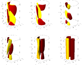
Figure 1: The NLOP at $Re=1750$ and $E_{0}=1.8\times 10^{-5}$ calculated using resolution (MM,NN,LL)=$(23,64,11)$ at $t=0$ (upper left), $t=0.4$ (upper middle), $t=1$ (upper right), $t=2.5$ (lower left), $t=5$ (lower middle) and $t=10\,D/U$ (lower right). Isocontours are shown of the streamwise perturbation velocity: yellow (light) 50% of the maximum and red (dark) 50% of the minimum. Mean flow in each pipe section is from bottom to top.

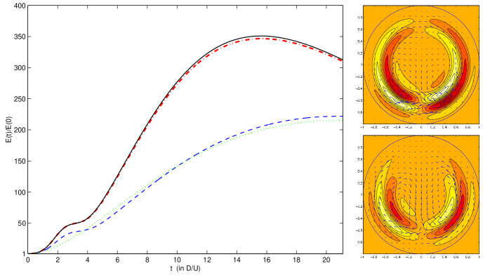
Figure 2: Left: energy growth $E(t)/E(0)$ against time $t$ for the NLOP of PK10 at Re=1750 and $E_{0}=1.8\times 10^{-5}$ using full resolution (MM,NN,LL)=$(23,64,11)$ (black solid line) and reduced resolutions $(7,64,1)$ (red dot-dash line) and $(2,64,1)$ (blue dashed line). Removing the helical mode effect by using resolution $(1,64,1)$ (green dotted line) destroys the NLOP to leave the LOP (notice the absence of a ‘shoulder’ in the curve at $T\approx 3\,D/U$). Right: NLOPs for $(7,64,1)$ (upper) and $(2,64,1)$ (lower). Contours indicate streamwise velocity perturbation (total velocity with the laminar state of equivalent mass flux subtracted off) using the same levels in both plots. Arrows indicate cross-sectional velocities (same scale used for both). Note that the slices are taken at the same point in the pipe but there may be a phase difference between the solutions as they are calculated using two different calculations. Also compare the slice for $(7,64,1)$ with that for $(23,64,11)$ given in the upper left of figure 4.

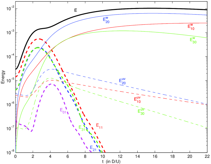
Figure 3: Modal energies for the NLOP run with resolution (7,64,1). $E$ is the total perturbation energy; $E_{ml}^{w}$ indicates the energy in the $w$ (streamwise) velocity component with azimuthal and axial wavenumbers $m$ and $l$ respectively, and $E_{ml}^{uv}$ the energy in the $u$ & $v$ (cross-stream) velocity components with azimuthal and axial wavenumbers $m$ and $l$ respectively. So $E_{m0}^{w}$ is the (streamwise) streak energy, $E^{uv}_{m0}$ is the (streamwise) roll energy and $E_{m1}$ is a helical mode energy.

A first inspection of the 3D structure of the evolving NLOP actually reveals 3 distinct phases of development. Figure 1 shows how the axial structure of the NLOP evolves in time by plotting isocontours of streamwise perturbation velocity along the pipe (isocontours of streamwise vorticity show the same qualitative behaviour). Initially the streaks are tightly layered and backward facing i.e. inclined into the shear. By $t=0.4$, these layers have been tilted into the mean shear direction (i.e. away from the wall) by the shear and unpacked or separated slightly. This is the inviscid Orr mechanism (Orr 1907) and gives an initial spurt of energy growth. By $t=1$ the flow is then dominated by helical waves growing - the ‘oblique’ phase - before the flow becomes essentially although not completely 2D by $t=10$ during the ‘lift-up’ phase. This evolution consisting of the Orr, oblique and lift-up phases in sequence is also apparently seen for the critical disturbance found by Monokrousos et al (2011) (D.S. Henningson, private communication).

To clarify the oblique and lift-up phases, we reduce the considerable degrees of freedom of the fully-resolved NLOP evolution down to those that really matter. As the Fourier-Fourier basis functions $\exp(im\phi+i\alpha lz)$ in the velocity representation naturally partition the linearized problem, we considered the optimal growth calculation at $Re=1750$, $T_{opt}=T_{lin}\approx 0.0122Re=21.3\,D/U$ in a pipe length of $\mbox{$\frac{1}{2}$}\pi D$ (so PK10 settings) at $E_{0}=1.8\times 10^{-5}$ using the full resolution (MM,LL)=$(23,11)$ and reduced resolutions $(7,1)$, $(2,1)$ and $(1,1)$ (full NN=$64$ radial resolution was used for all). Figure 2 shows how the growth evolves as a function of time for each optimal initial condition. All the calculations bar that for $(1,1)$ show the distinctive ‘shoulder’ in the growth centred at $t\approx 3\,D/U$ (the time units $D/U$ will be suppressed hereafter), which signifies the end of the (what PK10 called the ‘first’) delocalisation phase and the start of the next phase. The $(1,1)$ calculation fails to capture the NLOP at all so that the optimal that emerges is just the nonlinear version of the LOP. It is also striking that the $(7,1)$ optimal is quantitatively so similar to the full $(23,11)$-optimal indicating that axial wavenumbers beyond the lowest are not important for this short pipe calculation. Drastically reducing the azimuthal resolution to just $(2,1)$ has a noticeable quantitative effect but still manages to preserve the qualitative features of the NLOP. In particular the $(2,1)$-optimal (right lower, figure 2) captures the essential structure of the $(7,1)$-optimal (right upper, figure 2) which is itself almost identical to the $(23,11)$-optimal (upper left of figure 4) (although no attempt has been made to match phases of the solutions along the pipe).

The temporal evolutions of the modal kinetic energies $E_{ml}(t)$ (defined as the kinetic energy associated with the Fourier-Fourier wavenumbers $m,l$) for the $(7,1)$ calculation are shown in figure 3 (the equivalent plot for the $(2,1)$ calculation is qualitatively similar but not shown). The modal energy for streamwise-independent velocities, $E_{m0}$, is further split into that associated with the streamwise velocity, $E^{w}_{m0}$, and that with the cross-plane velocities $u$ and $v$, $E_{m0}^{uv}$. Each modal energy can change because of three effects: input from the underlying basic state due to the non-normality of the linearised operator, loss due to viscous dissipation and either loss or gain through nonlinear mixing with the other modes. Generally, it is difficult to distinguish between these effects without explicitly monitoring the various terms in the Navier–Stokes equations. However, for streamwise-independent modes, the cross-plane energy $E^{uv}_{m0}$ cannot grow by non-normal effects so any energy gain must be the result of nonlinear input alone. This observation is crucial for interpreting figure 3, which shows that after the Orr mechanism has played out, the NLOP evolution is dominated by the non-normal energy growth of helical modes ($m,l\neq 0$) in the second phase ($0.4\lesssim t\lesssim 2.5$). As these modes grow quickly, they feed energy via their nonlinear interactions into the streamwise-independent modes as evidenced in the increase in $E^{uv}_{m0}$ over the interval $2\lesssim t\lesssim 4$. When the nonnormal energy growth of the helical modes runs out of steam (at $\approx 2.5$) they decline quickly through the combined effect of this nonlinear energy drain and viscous dissipation. Thereafter, the evolution is dominated by each streamwise-independent mode experiencing slow but sustained non-normal growth as the secularly-decaying streamwise rolls advect the mean shear to produce streaks — the well-known lift-up process. The uniform decay rates of the streamwise rolls indicates that there is minimal nonlinear energy mixing at this point at least in the cross-plane velocities. This is because they are insensitive to axial advection (e.g. $w\,\partial u/\partial z=0$) and the cross-plane velocities are so small. Figure 2 shows these two non-normal growth processes together with the Orr mechanism cooperate nonlinearly to produce a larger overall growth at $T_{opt}$ than separately. After the initial rotation and unpacking by the Orr mechanism, the helical modes grow but quickly run out of steam. They then dump their energy into the third streamwise-rolls-driving-streaks process, which is subsequently boosted to reach higher growth factors than otherwise.

Figure 4: The NLOP at $Re=1750$ and $E_{0}=1.8\times 10^{-5}$ calculated using resolution (MM,NN,LL)=$(23,64,11)$ at $t=0$ (top left and top middle so same velocity field shown but with different contour levels), $t=0.2$ (top right), $t=0.6$ (bottom left), $t=0.8$ (bottom middle) and $t=1\,D/U$ (bottom right). Contours indicate the streamwise velocity perturbation (total velocity with the laminar state of equivalent mass flux subtracted off) and the arrows indicate the cross-stream velocity at a fixed slice in the pipe. All plots except the top left have 10 contour levels between the extremes of the streamwise velocity perturbation at $t=1$ and cross-stream velocities similarly scaled. The top left plot uses 10 contours between the extremes of the streamwise velocity perturbation at $t=0$ with arrows automatically scaled.

Figure 5: The NLOP at $Re=1750$ and $E_{0}=1.8\times 10^{-5}$ calculated using resolution (MM,NN,LL)=$(23,64,11)$ at $t=1$ (upper left), $t=2.5$ (upper right), $t=4$ (lower left) and $t=10,D/U$ (lower right) and representation is as in figure 4. All plots have 10 contour levels between the extremes of the streamwise velocity perturbation at $t=10$ and cross-stream velocities similarly scaled and set by those at $t=2.5$. Note that the upper left plot indicates exactly the same velocity field as the lower right plot in figure 4 but using revised contour and arrow levels.

The fact that helical (or more generically ‘oblique’) waves grow best over short times and streamwise-independent flows grow larger but over longer times is well known (e.g. figure 8 of Farrell & Ioannou 1993, figure 4 of Schmid & Henningson 1994 and figure 5 of Meseguer & Trethen 2003). Furthermore, the scenario of oblique waves growing transiently, feeding their energy into streamwise rolls that then drive streamwise streaks (which then become unstable) has also been proposed before as an efficient bypass mechanism in Reddy et al. (1998) (called the ‘oblique wave scenario’). This general picture, or at least the first stages of it, appear to be confirmed here in the nonlinear growth problem. However, the initial localisation of the perturbation and how it ‘unwraps’ to give a final, large, predominantly streamwise-independent flow is a new feature born out of a need to cheat the starting (global) energy constraint. Figures 4 and 5 show how the structure of the NLOP across one (fixed) slice of the pipe evolves in time. The initial slice shown (upper left and again upper middle but rescaled) has a peak cross-plane speed of $\approx 0.02U$ concentrated in a tight vortex pair near the pipe wall and peak axial speed of $\approx 0.012U$. The delocalisation or ‘unwrapping’ is effectively completed by $t\approx 1$ when the peak cross-plane speed is essentially unchanged whereas the peak axial speed has grown to $0.06U$. Figure 5 (the upper left slice is a rescaled version of the lower right of figure 4) shows that both the cross-plane and axial speeds grow considerably in the interval $1\lesssim t\lesssim 2.5$ (peak cross-plane speed increases from $0.02U$ to $0.08U$ and peak axial speed from $0.06U$ to $0.13U$). In fact, by $t=2.5$ the initial energy has experienced most of its growth (a factor of $\approx 50$) and only a further magnification by $\approx 7$ follows in the next $\approx 20\,D/U$. In this latter period the cross-plane velocities manoeuvre the streak structure into place and then die away so that even by $t=10$, the predominantly streamwise-independent and axial flow has been established (peak cross-plane speed is $0.012U$ and peak axial speed $0.34U$ now). It is worth stressing that even at this point, the flow does not match the LOP (see plot $c^{{}^{\prime}}$ in figure 2 of PK10), which depends solely on the Fourier-Fourier basis function $\exp(\mathrm{i}\phi)$ and is strictly 2D, being streamwise-invariant.

4 Tracking the NLOP in PK10

As discussed in section 1, PK10 demonstrated how nonlinearity can qualitatively change the form of the optimal disturbance of a given initial energy which achieves the most energy growth over a fixed period. The new NLOP could not, however, be followed up to the initial energy level at which turbulence was triggered. We now revisit this situation armed with a more efficient and parallel code which allows higher resolution and more carefully refined steps in $\boldsymbol{\mbox{\boldmath$u$}}_{0}$ to be used.

In PK10, a short $\mbox{$\frac{1}{2}$}\pi D$ periodic pipe was adopted to minimise the axial resolution needed and the relatively short time period was taken equal to $T_{lin}$, the time for maximum energy growth in the linearised Navier-Stokes equations, to highlight the effect of nonlinearity. Working at $Re=1750$, PK10 report failing to converge for $E_{0}>2\times 10^{-5}$. Their best estimate for $E_{c}$ was $\mathscr{E}_{c}=6\times 10^{-5}$, the energy required to trigger turbulence when using a perturbation of the form $A\mbox{\boldmath$u$}_{3d}(\mbox{\boldmath$x$};E_{0}=2\times 10^{-5},Re=1750)$. With the new code using a resolution $(MM,LL)=(23,11)$ and $NN=64$ finite difference radial points as opposed to PK10’s $(MM,LL)=(14,5)$ and a 25 Chebyshev polynomial expansion radially, we were able to confirm PK10’s results for $E_{0}\leq 2\times 10^{-5}$ as well as continuing to converge up to $E_{0}=2.52\times 10^{-5}$. Above this point, the amount of growth grows sharply compared with the amount of growth produced by rescaling arguments (figure 6).

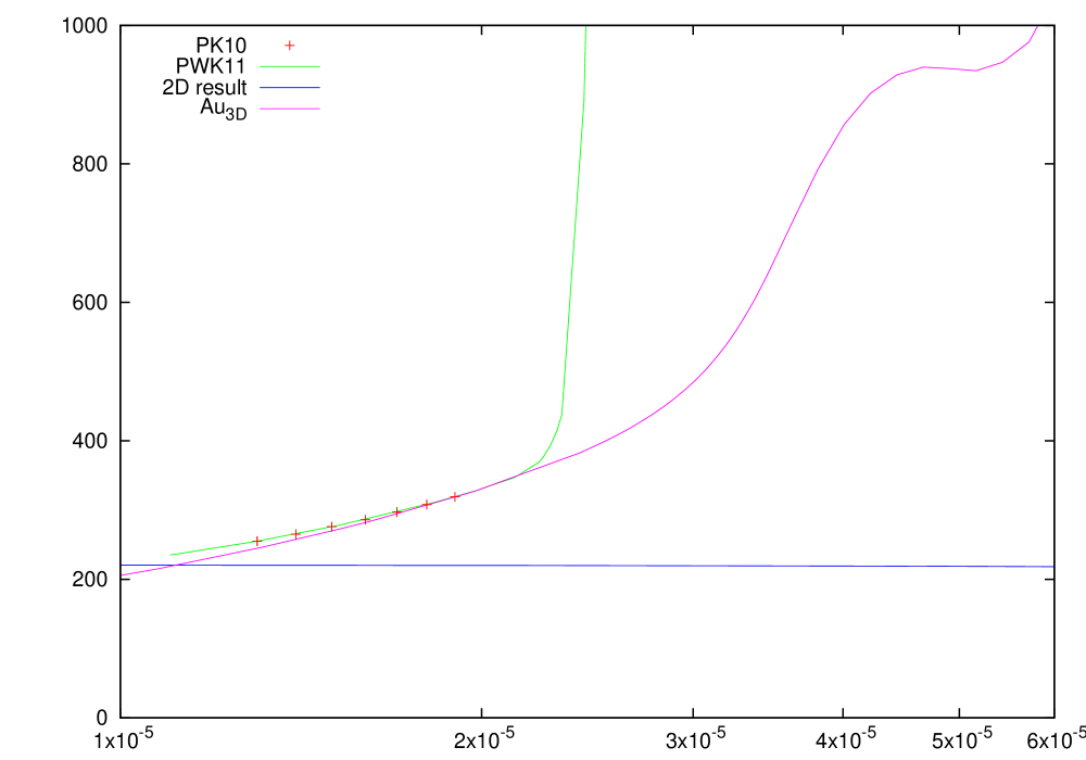
Figure 6: Reproduction of figure 5 from Pringle & Kerswell (2010) showing growth as a function of initial energy. The red crosses correspond to the nonlinear optimal perturbations previously calculated in PK10, while the (uppermost) green line represents the optimals calculated with the new code presented in this paper. The (middle) magenta line shows the amount of growth produced by simply rescaling the nonlinear optimal for $E_{0}=2\times 10^{-5}$ and therefore lower bounds the true (green) optimal growth curve. The (lowest) flat blue line is the growth provided by the nonlinearly modified 2D optimal (LOP).

Examining how the residual $\langle(\delta\mathscr{L}/\delta\mbox{\boldmath$u$}_{0})^{2}\rangle$ decreases as the algorithm proceeds indicates that the code has converged at $E_{0}=2.52\times 10^{-5}$: see figure 7 (outer). The time evolution of the optimal solution is relatively smooth, relaminarising after the initial transient growth. Surprisingly, however, one of the velocity fields it iterates through (marked with a black dot in figure 7, outer) does lead to a turbulent episode. A comparison of the two evolutions confirms the the optimisation procedure has worked properly: the optimal produces more growth than the other initial condition despite the fact it doesn’t lead to turbulence (figure 7, inner). This observation seems to go against our assertion that the optimisation algorithm will latch onto a turbulence-triggering state and then fail to converge. There are two important lessons to be learnt from this apparent pathology. The first, most obvious one is that the turbulence-triggering initial condition has not had enough time to reach the turbulent state by the end of the (short) period $T_{lin}$, so (1) $T_{opt}$ needs to be large enough. Secondly, figure 7 shows that the energy level reached by the optimal a little after $T_{lin}$ is actually higher than that typically associated with the turbulent state at this (low) $Re$ in this (tight) pipe geometry. This situation is fatal for the approach being advocated here, which relies on the turbulent state producing the highest values of the energy growth (or whatever functional is being considered) in comparison to non-turbulent states. Fortunately, such a situation only seems to occur in tightly-constrained (small geometry) flows close to (in $Re$) the first appearance of the turbulent state. Therefore, the second lesson is that (2) the optimisation strategy can only be used sufficiently far from the first appearance of turbulence and/or for flows in large domains.

In hindsight then, the geometry and $Re$ value chosen in PK10 is not suited for determining $E_{c}$ there using this optimisation approach. We therefore switch to a longer $5D$ periodic pipe (theoretically popular since the work of Eggels et al. 1994) and a higher $Re=2400$ where the edge shows typical behaviour (Duguet, Willis & Kerswell 2008) and the turbulent state is clearly energetically separated from the edge state (e.g. Schneider & Eckhardt 2009, figure 7).

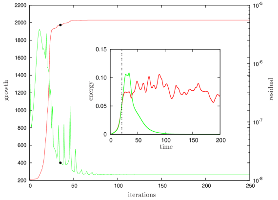
Figure 7: Convergence of procedure at $E_{0}=2.52\times 10^{-5}$. The algorithm smoothly converges to a growth of 2030 (upper right line), while the residual decays to $O(10^{-8})$ (lower right line). The algorithm was continued for over 800 iterations in total to ensure that there was no further change. Inset: The time evolutions of two disturbances found by this sequence of iteration. The green (lower right) line is the converged optimal which smoothly relaminarises, while the (upper right) red line is the disturbance corresponding to the black dot leading to a turbulent episode. The vertical dashed line shows the target time $T_{opt}=T_{lin}\approx 21.3\,D/U$ from the optimisation procedure.

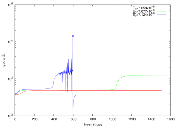
Figure 8: The amount of growth produced by successive choices for $\mbox{\boldmath$u$}_{0}$ in the interative scheme. For $E_{0}=7.058\times 10^{-6}$ the growth plateaus out at 483 (red lower line). For $E_{0}=7.124\times 10^{-6}$, the growth briefly plateaus at $\sim 520$ before rapidly rising to excess of $1,000$ (upper blue line). The circle plotted shows a growth of $14,480$ and has reached the turbulent attractor before the algorithm steps momentarily back to a region below the edge. The turbulent seed and the optimal for $E_{0}=7.058\times 10^{-6}$ are both plotted in figure 18. Before this has been reached, however, the growth being produced is already nonsmooth between steps due to the lack of smoothness in the hypersurface $\mathscr{L}$, as predicted by conjecture 1. We also include the choice of $E_{0}=7.077\times 10^{-6}$ for illustrative purposes (middle green line). This iterative run has not been fully converged and it is not clear whether it will converge to an optimal or depart to the turbulent state.

5 Long Time and a $5\,D$ Pipe

In order to assess the twin conjectures discussed in section 1, a practical decision needs to be made as to what constitutes a ‘asymptotically long’ optimisation time. Figure 7 shows that an initial condition is capable of growing through several orders of magnitude into a turbulent epsiode within $\sim 50\,D/U$. We therefore chose $T_{opt}=75\,D/U$, which should be large enough to capture this behaviour especially in a larger $5D$ domain although $Re=2400$ is higher (so $T_{opt}>2.5T_{lin}$ at this $Re$). It is worth remarking, though, that this finite choice will limit the accuracy to which we can determine the energy threshold. The algorithm senses initial conditions which have reached the turbulent state by the end of the observational window. This sets a lower limit on how close they can be to the edge, as the time for a turbulence-triggering initial condition to reach turbulence becomes arbitrarily large as it is taken closer to the edge. This said, our choice of $T_{opt}$ gives acceptable accuracy yet the way to improve this is clear through integrating for longer.

The results of the energy growth optimisation in a $5\,D$ pipe at $Re=2400$ as a function of $E_{0}$ exactly mimicks the situation uncovered in PK10. For $E_{0}$ small enough, the linear (streamwise-independent) optimal (LOP) is selected albeit with slight nonlinear modification, which suppresses the growth of the 2D optimal as $E_{0}$ increases. Then there is a finite value (PK10 refer to this as $E_{3d}$) when a new 3D optimal (NLOP) is preferentially selected, which shows localisation in the azimuthal and radial directions. There is also some localisation in the streamwise direction, however the domain is by no means long enough for us to observe truly localised optimals as opposed to periodic disturbances.

As $E_{0}$ is increased further, there comes a point at which the algorithm struggles to converge properly. Successive bisection indicates that this value, $E_{fail}$, is bracketed by the initial energy values of $E_{0}=7.058\times 10^{-6}$ which converges smoothly to the NLOP and $7.124\times 10^{-6}$ which clearly fails due to the occurrence of a turbulence-triggering initial condition: see figures 8, 9 and 10.

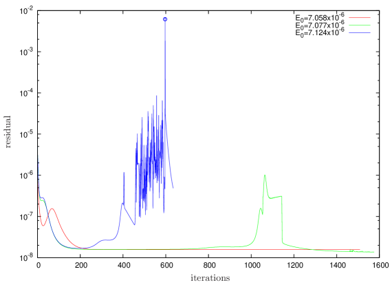
Figure 9: The residuals corresponding to the three iterative runs described in figure 8 (flat red line $7.058\times 10^{-6}$, green line with spike at $1100$ $7.077\times 10^{-6}$ and upper blue $7.124\times 10^{-6}$). The sudden adjustment centred on 1100 iterations is a warning that deciding upon convergence can be a subtle affair.

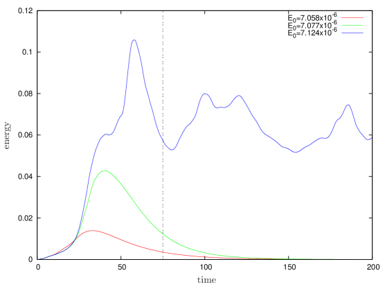
Figure 10: Evolution of the final states produced by the iterative scheme for $E_{0}=7.058\times 10^{-6}$ (red lowest line) and $7.124\times 10^{-6}$ (blue uppermost line). One clearly leads to a turbulent episode while the other simply relaminarises after the intial transient growth. Also shown is the evolution of the initial condition arrived at after 1600 iterations for $E_{0}=7.077\times 10^{-6}$ (middle green line) which again relaminarises. The vertical line marks the optimisation time.

An attempt to improve this bracketing by taking $E_{0}=7.077\times 10^{-6}$ appears to show convergence yet there still remains some doubt even after running the algorithm for nearly 1600 iterations and 50,000 CPU hours ($\approx 6$ years). Figure 8 indicates convergence yet at a much higher level compared to that reached by the ‘nearby’ initial energy of $E_{0}=7.058\times 10^{-6}$. Moreover the fact that there is a jump up to this higher level after $\approx 1000$ iterations is mildly disconcerting. This adjustment is reflected in the evolution of the residual (see figure 9), which after $200$ interations, appears to show convergence for the next $500$ iterations before being followed by a rapid transition that ends after $1150$ iterations. It is not clear whether the algorithm now has finally converged or whether it will subsquently encounter a turbulence-inducing initial condition. This example demonstrates that it is clearly very important to take care when deciding whether the procedure has converged or not (e.g. stopping the algorithm after 600 iterations would indicate clear convergence). It is probable that the algorithm is struggling to discern between turbulence-inducing initial conditions and the NLOP because the time to reach turbulence is comparable to, or exceeds, $T_{opt}$. Consequently, the estimate that $7.058\times 10^{-6}<E_{fail}<7.124\times 10^{-6}$ is the best we can hope for working with $T_{opt}=75\,D/U$ and the fate of $E_{0}=7.077\times 10^{-6}$ could be decided by taking a longer $T_{opt}$ (not pursued here).

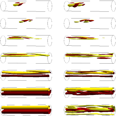
Figure 11: Snap shots showing isocontours of streamwise perturbation velocity during the evolution of the final states produced by the iterative scheme for $E_{0}=7.058\times 10^{-6}$ (left) and $7.124\times 10^{-6}$ (right). The isocontours in each plot correspond to $50\%$ of the maximum (light yellow) and $50\%$ of the minimum (dark red) of the streamwise perturbation velocity in the pipe at that time. The snapshots correspond to times $t=0$, $0.5$, $5$, $10$, $20$, $40$ and $75\,D/U$. In both cases the energy is initially localised in the streamwise direction and the disturbance quickly spreads. By $t=10$ both disturbances have created streamwise streaks but only for the lower energy do they become streamwise independent. The larger amplitude of the higher energy streaks are subject to a turbulence-triggering instability.

The physical evolution of the two disturbances is shown in figure 11. Initially the disturbances look streamwise-localised because of the contouring but they do in fact occupy the full length of the domain. Both subsequently develop into coherent domain-length streaks. In the $E_{0}=7.058\times 10^{-6}$ case, these streaks continue to evolve yet remain stable, becoming almost totally streamwise-invariant before ultimately decaying. In the $E_{0}=7.124\times 10^{-6}$ case, the streaks have higher amplitude and a streak instability clearly occurs leading to turbulence. The nature of this instability is shown in figure 12 which plots the streamwise dependent and independent components of the energy of the axial velocity field with (lead) azimuthal wave number $m=1$. For the relaminarising disturbance, the 3D part of the energy decays monotonically from around $15\,D/U$ onwards. For the more energetic disturbance the decay is abated after $20\,D/U$ at which point, an instability of the streaks occurs eventually leading to turbulence. It is worth remarking that the final plot for $E_{0}=7.058\times 10^{-6}$ in figure 11 resembles more the two streaks produced by the linear optimal, rather than the three-streak field generated in PK10 (cf figure 5, bottom right in this paper). Whether this is due to the increased target time or the lengthened flow domain is unclear.

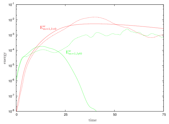
Figure 12: The energy associated with the $m=1$ axial component of the disturbances calculated for $E_{0}=7.058\times 10^{-6}$ (solid) and $E_{0}=7.124\times 10^{-6}$ (dashed). Each energy is split into streamwise-independent (dark red uppermost lines at $t=25D/U$) and streamwise-dependent (light green lowermost lines at $t=25D/U$) parts. The former measures the streaks created by the disturbance while the latter shows the instability of these streaks.

Conjecture 1 claims $E_{c}=E_{fail}$. As there is no evidence of turbulence-triggering initial conditions at $E_{0}=7.058\times 10^{-6}$ but there is at $7.124\times 10^{-6}$, we have $7.058\times 10^{-6}<E_{c}<7.124\times 10^{-6}$. To this level of accuracy we have found that $E_{c}=E_{fail}$. That the optimisation scheme will fail if turbulent seeds exist within the $E_{0}$-hypersurface seems clear provided the iterative scheme can find them. Establishing this is very difficult if not impossible, but a weaker practical alternative is to demonstrate that the procedure is not dependent on the initial starting guess $\mbox{\boldmath$u$}_{0}$. To do this we have compared six very different choices for the initial seed for both $E_{0}<E_{fail}$ and $E_{0}>E_{fail}$ and plotted their evolution on a 2D projection of energy in the axisymmetric part of the perturbation against energy in the streamwise-independent part (figures 13 and 14). The scatter of the initial crosses illustrates the variety of initial conditions used which range from turbulent velocity fields to known travelling wave solutions. In both cases, irrespective of where the scheme begins, the eventual (iterative) evolution brings it to the same trajectory in this ‘phase space’. This provides some evidence that the algorithm does sample the $E_{0}$-hypersurface well and that Conjecture 1 indeed holds true.

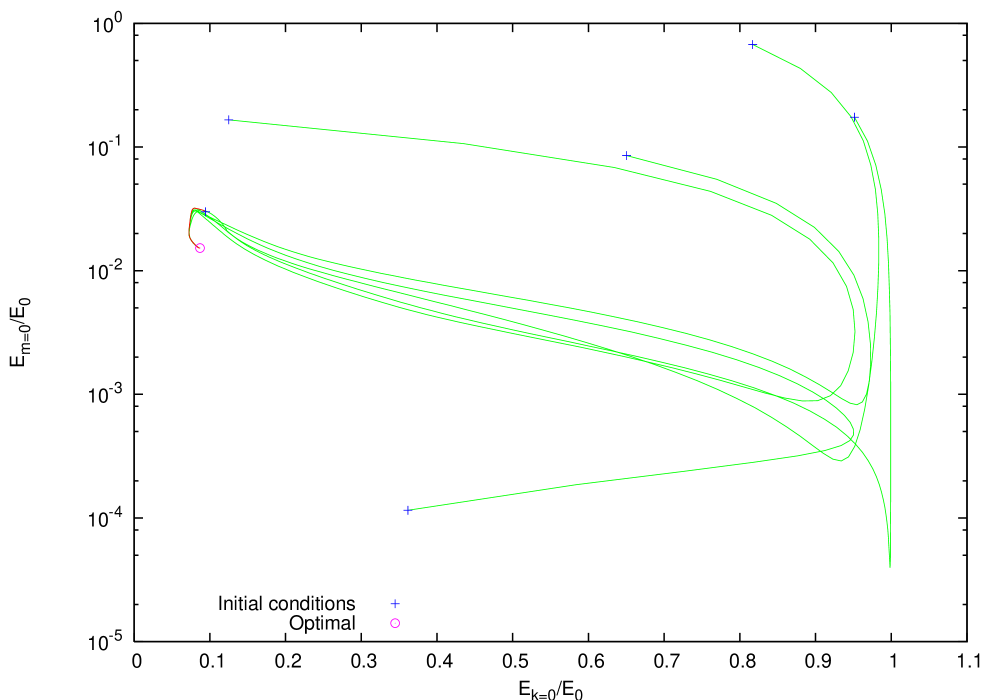
Figure 13: Convergence of six different initial conditions (crosses) towards the same optimal (circle) for $E_{0}=7.058\times 10^{-6}$: axes are normalised perturbation energies associated with the streamwise-independent part (abscissa) and the axisymetric part (ordinate). The initial conditions chosen correspond to the various combinations of turbulent flow fields, travelling wave solutions and the nonlinear optimal from section 4. The red line corresponds to this final choice and is the iterative scheme shown in figures 8 and 9.

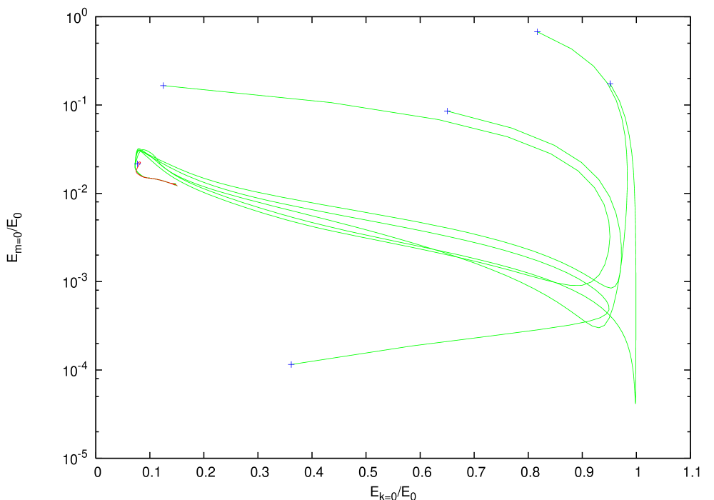
Figure 14: The result of using the same six initial conditions (crosses) for $E_{0}=7.124\times 10^{-6}$. The red line corresponds to the iterative progression shown in figures 8 and 9. Clearly, the procedure is independent of the starting guess. Note also how similar the progression is here to that for $E_{0}=7.058\times 10^{-6}$.

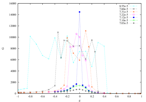
Figure 15: Growth factors in the neighbourhood of the seed state $\mbox{\boldmath$u$}_{t}$ that triggers turbulence at $E_{0}=7.124\times 10^{-6}$. The neighbourhood is defined by $d$ where $\mbox{\boldmath$u$}_{ic}(\mbox{\boldmath$x$};d):=A[\,(1+d)\mbox{\boldmath$u$}_{l=0}+(1-d)\mbox{\boldmath$u$}_{l\neq 0}\,]$, $\mbox{\boldmath$u$}_{l=0}$ is the streamwise-independent part of $\mbox{\boldmath$u$}_{s}$ and $\mbox{\boldmath$u$}_{l\neq 0}:=\mbox{\boldmath$u$}_{s}-\mbox{\boldmath$u$}_{l=0}$. The amplitude $A$ is used to rescale the initial state to ensure the correct starting energy $E_{0}$. The figure shows that $\mbox{\boldmath$u$}_{s}$ only just triggers transition at $7.124\times 10^{-6}$ but for higher energies, an ever-increasing neighbourhood of initial conditions surrounding $\mbox{\boldmath$u$}_{s}$ exists which trigger transition (indicated by the jump in $G$).

In order to assess Conjecture 2, we now consider the behaviour of the optimal solution close to the edge. Figures 13 and 14 already provide some evidence that the NLOP at $7.058\times 10^{-6}$ and the turbulent seed found at $7.124\times 10^{-6}$ are similar at least in terms of their axisymmetric and streamwise-independent energy fractions. In order to probe the accuracy of Conjecture 2 further, we look at the one initial condition that in section 5 our algorithm identified for $E_{0}=7.124\times 10^{-6}$ that was a turbulent seed, $\mbox{\boldmath$u$}_{s}$ (indicated by the circle in figure 8) . The fact that only the one condition was found above the edge of chaos suggests that in this region there is only a very small set of turbulence-triggering initial conditions. We attempt to quantify this by considering the evolution of initial conditions of the form

$$\mbox{\boldmath$u$}_{ic}(A,d):=A[(1+d)\mbox{\boldmath$u$}_{l=0}+(1-d)\mbox{\boldmath$u$}_{l\neq 0}]$$ (14)

where $\mbox{\boldmath$u$}_{l=0}$ and $\mbox{\boldmath$u$}_{l\neq 0}$ are the streamwise independent and dependent parts of $\mbox{\boldmath$u$}_{s}$ and $A$ is adjusted to give the required value of $E_{0}$. The amount of growth after $75D/U$ is shown as a function of $E_{0}$ and $d$ in figure 15. The jump in growth from $O(10^{3})$ to $O(10^{4})$ clearly demarcates where the edge of chaos is crossed. The narrowness of the peak for $E_{0}=7.124\times 10^{-6}$ and the observation that a mere $\sim 0.3\%$ reduction in amplitude is enough to dip beneath the edge, indicates that $\mbox{\boldmath$u$}_{s}$ is very close to a local minimum of the edge. The precise energy at which $\mbox{\boldmath$u$}_{ic}(A,d=0)$ crosses the edge is plotted in figure 16. Here two bracketing cases are shown: $E_{0}=7.121011\times 10^{-6}$, which ultimately relaminarises, and $E_{0}=7.121019\times 10^{-6}$, which leads to turbulence. The closeness of these energies means that both evolutions track the edge to $T\approx T_{opt}$ before going their separate ways. This emphasizes that to improve the estimate of $E_{c}$ discussed above, $T_{opt}$ has to be increased.

Coincidentally, while following the relaminarising case, the flow was found to transiently resemble the asymmetric travelling wave believed to be embedded in the edge state (Pringle & Kerswell 2007, later named $S1$ in Pringle et al. 2009) at $t\approx 100\,D/U$. This was verified by calculating the two correlation functions, $I_{tot}$ and $\mbox{$\frac{1}{2}$}(I_{tot}+I_{uv})$, introduced in Kerswell & Tutty (2007, definitions (2.3) and (2.5)). Figure 17 shows that both these correlations simultaneously exceed 0.75 at $t\approx 100\,D/U$ clearly indicating a very close ‘visit’ (0.6 was deemed good enough to indicate a ‘close’ visit by Kerswell & Tutty 2007). The fact that this visit takes place is not a surprise but more a check of consistency: the edge state is believed unique and therefore a global attractor on the edge at this $Re$ and pipe length (Schneider, Eckhardt & Yorke 2007). It is worthy of note, however, that it takes a comparatively long time of $\approx 100\,D/U$ for a flow trajectory starting at the lowest energy point on the edge to reach the $S1$ state.

Examining the NLOP for $E_{0}=7.058\times 10^{-6}$ and $\mbox{\boldmath$u$}_{s}$, it seems reasonable to conclude that the minimal seed of turbulence is ‘sandwiched’ in between. The form of the two solutions are shown in figure 18 (along with the last iterate calculated at $7.077\times 10^{-6}$) and it is clear that they don’t alter much as the edge is crossed. This supports Conjecture 2.

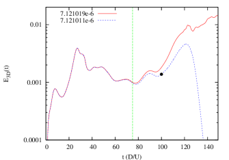
Figure 16: Trajectories close to the laminar-turbulent boundary, or ‘edge’. Nearby initial conditions are $\mbox{\boldmath$u$}_{ic}=A\mbox{\boldmath$u$}_{s}$, with $A$ selected to give the indicated energies. The case $E_{0}=7.121011\times 10^{-6}$ relaminarises but not before passing close by the edge attractor (marked by the dot which is the energy of the $S1$ travelling wave embedded in it). The case $E_{0}=7.121019\times 10^{-6}$ tracks the edge before leading to turbulence, The vertical line is $T=T_{opt}=75D/U$.

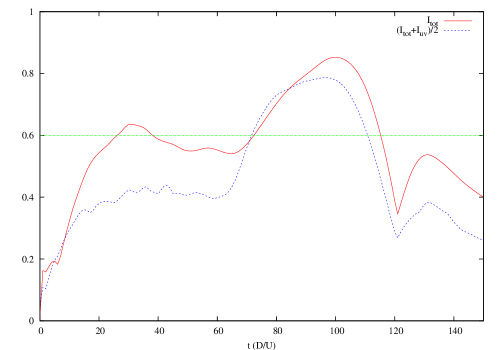
Figure 17: Correlation function data which measures how close the instantaneous velocity field is to the asymmetric travelling wave $S1$ for the trajectory which relaminarises in figure 16 with $E_{0}=7.121011\times 10^{-6}$. The fact that $I_{tot}$ and $\mbox{$\frac{1}{2}$}(I_{tot}+I_{uv})$ exceed $0.75$ at $t=100\,D/U$ indicates a very close visit (Kerswell & Tutty 2007). The importance of this visit is that $S1$ is believed embedded in the chaotic edge state for the pipe length and $Re$.

Figure 18: The nonlinear optimal calculated in section 5 for $E_{0}=7.058\times 10^{-6}$ (left) and the turbulent seed $\mbox{\boldmath$u$}_{s}$ (right). The close similarity between the two solutions is striking with the turbulent seed having stronger streaks but an otherwise comparable structure. For comparison we have also included the final state found for $E_{0}=7.077\times 10^{-6}$ (middle). This state appears to be an intermediary between the two other states.

6 Discussion

We first summarise what has been done in this paper. An exploratory nonlinear energy growth calculation in PK10 showed that the form of the optimal initial disturbance changes suddenly at a small (pre-threshold) but finite initial energy level $E_{3d}$ from a global linear optimal (weakly modified by nonlinearity) to a localised strongly nonlinear optimal. This has been confirmed at higher spatial and temporal resolution. The physical processes responsible for the enhanced energy growth of the new nonlinear optimal (NLOP) have been identified as three known linear growth mechanisms — the Orr mechanism, oblique wave transient growth and the lift-up effect — acting sequentially and coupled together via the nonlinearity of the Navier-Stokes equations. These mechanisms operate on differing timescales yet appear able to pass on their growth to the next (slower) process so that the total growth outweighs any of their individual contributions. The NLOP is also localised, which is an inherently nonlinear feature designed to cheat the global initial energy constraint. The calculations here have also managed to converge this nonlinear optimal state beyond the threshold energy level at which turbulence could be triggered. This highlighted two issues for the optimisation strategy to identify this energy threshold: 1) the optimisation time needs to be large enough that turbulence-triggering initial conditions have time to reach the turbulent state; and 2) the energy levels of the turbulent state need to be above those for laminar flows so that the optimisation algorithm will naturally seek them out. This indicates that the optimisation strategy discussed here is better suited to larger flow domains and more supercritical (higher $Re$) regimes. Ironically, it is now clear that doing exploratory (cheap) calculations in a small domain at low $Re$ was a natural but bad choice in PK10.

Calculations in a longer pipe 5D at higher $Re$ (=2400) over a larger time period found the same general situation as in the $\mbox{$\frac{1}{2}$}\pi D$ pipe of PK10. At low initial energies, the optimal is the (global) linear optimal weakly modified by nonlinearity. At a certain small but finite initial energy $E_{3d}$, a new localised 3D optimal (NLOP) is preferred, which stays the optimal until the algorithm fails to converge at $E_{fail}$. The only significant difference is that in the longer $5D$ pipe, the NLOP is starting to streamwise-localise in contrast to the $\mbox{$\frac{1}{2}$}\pi D$ NLOP, where the shortness of the domain prevents this. Above $E_{fail}$, initial conditions that trigger turbulence are found to exist on the energy hypersurface and to the accuracy available, $E_{fail}=E_{c}$. This supports Conjecture 1, which presupposes that the optimisation algorithm will find any turbulent-triggering states if they exist on the energy hypersurface and then fail to converge as a result. As way of confirming this, the algorithm was tested with a variety of very different starting conditions with the same optimal emerging, indicating that the optimisation algorithm is able to explore the energy hypersurface.

Intriguingly, good evidence was also found that NLOP $\rightarrow$ minimal seed as $E_{0}\rightarrow E_{c}^{-}$ in support of the stronger Conjecture 2 at least for this flow, geometry and $Re$. Pictorially, this means that the NLOP for $E_{c}$ and the minimal seed actually coincide in figure 19 rather than the more general situation shown where the two differ (for clarity). It was also argued that, with enough computational power, the threshold energy $E_{c}$ and the minimal seed could be calculated to arbitrary accuracy by increasing the spatial and temporal resolution as well as $T_{opt}$, which improves the algorithm’s ability to discern between trajectories that become turbulent and those that relaminarise.

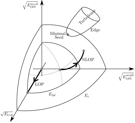
Figure 19: Cartoon to illustrate Conjectures 1 and 2. Conjecture 1 asserts that the optimisation approach will yield a well-defined nonlinear optimal (NLOP) up until $E_{0}=E_{c}$ whereupon turbulence can be triggered by the minimal seed. Conjecture 2 asserts that the NLOP converges as $E_{0}\rightarrow E_{c}^{-}$ to the minimal seed (the converse situation where the limiting NLOP state and the minimal seed are different is shown for clarity). Note the LOP is streamwise-independent in pipe flow and hence traces the $E_{l=0}$ axis.

The strategy advocated here for determining the minimal finite amplitude disturbance to trigger transition to turbulence in shear flows involves constructing and iteratively solving a variational problem. The objective functional must be selected such that it identifies turbulent velocity fields by taking enhanced values compared to those for laminar fields. This is then maximised via searching over all incompressible disturbances of fixed amplitude that respect the boundary conditions over an asymptotically long time period constrained by the full Navier-Stokes equations. All of the results discussed here have been obtained using the perturbation energy growth over a given period as the key functional. This certainly takes enhanced values for turbulent velocity fields in the 5D pipe at $Re=2400$ and Conjecture 1 seems to hold true. However, other choices should also work equally well, e.g. the total dissipation (Monokrousos et al. 2011), provided they share this crucial property. If Conjecture 1 is indeed true, then the optimisation strategy discussed here will identify the threshold energy level $E_{c}$. However, more is available too, albeit indirectly, as the minimal seed should be the unique initial condition that triggers turbulence as $E_{0}\rightarrow E_{c}^{+}$. Given this, the status of Conjecture 2, although conceptually fascinating, seems less important practically. Whether or not Conjecture 2 holds for energy growth (and, admittedly, we only have one supportive data analysis here), it can of course be restated for any functional. Then the question really is: is there a universal functional that when optimised always identifies the minimal seed as $E\rightarrow E_{c}^{-}$ for a class of flows (e.g. wall-bounded shear flows)? This seems unlikely to be exactly true but nevertheless may be approximately true for some subset of functionals. Then any of these could give acceptable predictions depending on how the results are to be subsequently used (e.g. designing disturbances in the laboratory). Certainly this would seem to be the case using the energy growth functional given the comparison in figure 18.

The variational approach espoused here is, of course, incredibly flexible. Changing the key functional is straightforward as is the initial (norm) constraint on the competitor initial fields. Although the discussion above has concentrated on the initial perturbation energy $E_{0}$, it should be clear other norm choices can be made. Providing the functional under consideration jumps to large values for turbulent flows, the optimisation algorithm should converge up until the first point (as the norm hypersurface ‘expands’ away from the laminar state) at which the edge penetrates the hypersurface (as per Conjecture 1). Furthermore, the turbulent state does not have to be the only target of the approach. Identifying the peak instantaneous pressure in a transitional flow is a key concern for pipeline structural integrity. One could easily imagine formulating an optimisation problem to maximise the pressure after time $T_{opt}$ over all disturbances of initial energy $E_{0}$ where $T_{opt}$ is also part of the optimisation procedure.

The long term objective of this theoretical work is to design better (lower energy) ways to trigger turbulence with a view to informing control techniques. Further calculations clearly need to be carried out in more realistic geometries to see, for example, if universal localised minimal seeds emerge. Even now though, this work is in a position to stimulate new experiments. The NLOP identified here indicates that structures that initially point into the shear will outgrow the equivalent structure directed across the shear (the Orr mechanism). This suggests a modification of the recent experiments of Peixinho & Mullin (2007) which were designed to generate oblique rolls by blowing and sucking directly across the shear. The calculations performed here indicate that their threshold scaling exponent (a non-trivial flux $\sim Re^{-1.5}$) for transition may possibly be further reduced if the blowing and sucking is inclined upstream to take advantage of the Orr mechanism.

7 Glossary

$E_{0}$	initial energy of a perturbation
$E_{T}$	final energy of a perturbation after time T
$E_{3d}$	initial energy at which the NLOP first emerges as the new optimal
$E_{fail}$	the minimum energy for which the optimisation routine fails to converge
$E_{c}$	the critical energy corresponding the minimum energy of the edge
$\mathscr{E}_{c}(\mathbf{u})$	the minimum energy of a perturbation of the form $A\mathbf{u}$ required to trigger turbulence
$T_{opt}$	the target time in an optimisation procedure
$T_{lin}$	the time for which transient growth is maaximised in the linear problem
$T_{turb}$	typical time period required for the onset of turbulence
$\mathbf{u}_{2D}(\mathbf{x};Re,E,L,T)$	the two dimensional optimal for the Reynolds number, energy, domain length and optimisation time T specified
$\mathbf{u}_{3D}(\mathbf{x};Re,E,L,T)$	the three dimensional optimal for the Reynolds number, energy, domain length and optimisation time T specified