Nonlinear spectroscopy of superconducting anharmonic resonators

Abstract

We formulate a model for the steady state response of a nonlinear quantum oscillator structure, such as those used in a variety of superconducting qubit experiments, when excited by a steady, but not necessarily small, ac tone. We show that this model can be derived directly from a circuit description of some recent qubit experiments in which the state of the qubit is read out directly, without a SQUID magnetometer. The excitation profile has a rich structure depending on the detuning of the tone from the small-signal resonant frequency, on the degree of damping, and on the excitation amplitude. We explore two regions in detail: First, at high damping there is a trough in the excitation response as a function of detuning, near where the classical Duffing bifurcation occurs. This trough has been understood as a classical interference between two metastable responses with opposite phase. We use Wigner function studies to show that while this picture is roughly correct, there are also more quantum mechanical aspects to this feature. Second, at low damping we study the emergence of sharp, discrete spectral features from a continuum response. We show that these the structures, associated with discrete transitions between different excited-state eigenstates of the oscillator, provide an interesting example of a quantum Fano resonance. The trough in the Fano response evolves continuously from the “classical” trough at high damping.

I introduction

Spectroscopic studies of superconducting qubit systems have increased steadily in sophistication in recent years. For many of the first Josephson-junction qubits, their only link with the outside world was magnetometry: diamagnetic currents, particularly in flux qubits, were detectable by SQUID magnetometers. While this provided the basis for some of the first experiments in which solid state qubit states were detected, these magnetometers were very intrusive devices in these systems, and were clearly an impediment to scalable systems. Spectroscopy with these SQUID detectors was very limited.

With the application in recent years of many sophisticated techniques from microwave engineering, various alternatives to the SQUID approach have emerged. The detection, protection, and manipulation of superconducting qubits have undergone impressive improvements. In particular, the spectroscopic probing of qubits and qubit/resonator systems is now capable of very useful high-fidelity qubit detectionSQUIDless ; TroughExpt , as well as detailed characterization of the parameters of these systems opening a beautiful view TroughTheory into the rich quantum response that these systems exhibit.

This paper will provide a theoretical study of a model that is central to these spectroscopic studies. The model is that of a single oscillator (bosonic mode) with a purely quartic anharmonicity. The oscillator is driven by a single ac tone, which is not necessarily a small perturbation on the system, and the system is damped with a purely frictional term, representative of a zero-temperature quantum environment. The observable is taken to be essentially the displacement of this resonator.

We will emphasize here the insights that can be gained from analytic or semi-analytic studies of this model. In previous studies of this modelDW , it has been shown that the steady state response of the system can be calculated in closed form. It is very rewarding to look at the many aspects of this amazingly rich solution. At high damping it exhibits much of the phenomenology of the classical Duffing oscillator. In a broad region of detuning, on the “red” side of the harmonic response frequency, and for moderately high amplitude excitation, the response is “high”, or quasi-resonant. But as damping is decreased, new, sharp resonant structures emerge from the broad Duffing feature. These lines are clearly associated with individual spectroscopic transitions in the anharmonic ladder of energy eigenstates. But the line shapes of these new lines are very non-Lorentzian, and are indicative of a complex interaction among different response channels.

In the present work we do further calculations to gain more understanding of several of these spectroscopic features. Up to a point, the behavior in the high damping regime exactly matches the classical Duffing theory. There is a linear response regime, in which the response is a simple Lorentzian centered on the harmonic frequency of the oscillator; at higher excitation amplitude the resonant line moves to lower frequency and sharpens. But there are differences: the quantum model intrinsically does not have multiple solutions for the steady state response, and so does not have any hysteretic behavior. Near the classical bifurcation point the quantum response shows a fairly abrupt transition, as a function of excitation detuning, between a “low” and “high” response regime.

While some details of this interesting quantum behavior have been discussed in previous work, we shed new light on this behavior using simple Wigner function computations. In the middle of this transition from “low” to “high” response, there is a dip in the response amplitude, which has been interpreted DW ; TroughTheory as a kind of intermittency in the steady state involving two responses with different, and therefore canceling, phases. Our Wigner functions show that there is clearly some truth to this point of view, but we find that, even for damping large enough to wash out all other quantum spectral features, the dip has more features than can be explained by any classical intermittency point of view. We find that this story is considerably enriched by using some of the modern tools of quantum information theory, such as calculations of the von-Neumann entropy, and some basic facts about the eigenanalysis of the completely positive map describing time evolution in our model.

We also explore in detail how structure emerges as the damping parameter is decreased. While the spectral response grows considerably in complexity, we find that the simple “dip” described above in the high damping regime persists for all values of damping, but comes in a different guise in this quantum limit. In one part of the spectrum, we identify this dip as a feature of a Fano resonance. The Fano phenomenon is a quintessentially quantum interference, yet we find that in this case it is one extreme of a family of interference phenomena that also include a nearly classical form of interference at the other extreme.

These studies help us to answer a very fundamental question about anharmonic resonant structures, which is: when is it reasonable to call such a structure a qubit? It is evident that the answer is a dynamical one: the very same resonator can be either a very well defined two-level quantum system (a qubit), or an oscillator requiring a many-level quantum description, depending on the amplitude and frequency of oscillation. In this paper we will fairly precisely demarcate the rather complex boundary between these two regimes.

II the electrical device

II.1 Circuit basics

The calculations here are motivated by current experiments on superconducting circuits such as the one shown in Fig. 1. The ac voltage signal (in the microwave frequency range, in cases of current interest) excites a transmission line; this transmission line is coupled capacitively to a small, discrete superconducting circuit that we will, for short, call “the qubit.” But an important message of this paper is that structures of interest do not always behave as qubits, that is, like two-level quantum mechanical systems. From the point of view of electrical science, the combination shown of a capacitor, inductor, and Josephson junction is viewed as an anharmonic resonator. As we will show, depending on the excitation conditions, this classical view is sometimes more appropriate than the quantum mechanical one. In fact, there is a rich set of phenomena that are explained by neither the classical or the simple (two-level) quantum point of view.

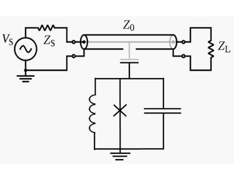
Figure 1: Experimental schematic.

Many features of a real experiment are omitted from Fig. 1. Naturally the qubit is held at low temperature, while the microwave voltage source is (presently) always at room temperature; the diagram does not show the attenuator stages that are necessary to keep room temperature noise out of the qubit. But these stages are engineered so that the functioning is that of a cold, matched (i.e., $Z_{S}=Z_{0}$) source. On the output end, conceptually measurements of the qubit are recorded as the voltage across the terminating resistor $Z_{L}$. In reality, this circuit is a complex, active chain of amplifiers and other components, with a signal recorded at room temperature. But again, the engineering of this chain has the object of reducing the effective functioning to that of the simple circuit in Fig. 1, in which the load is matched ($Z_{L}=Z_{0}$) and cold.

Much experiment and analysis (cf. saturatetoo ) has been devoted to a related circuit, in which the transmission line is only weakly (capacitively) coupled to the source and load circuits. This is the “circuit QED” setting, in which the transmission line forms a resonator which functions as a quantum-coherent resonator. The combination of this quantum resonator and the qubit exhibits rich, interesting, and potentially useful physics. The system we analyze here does not have all the same potentialities as the cQED system, but its dynamics still has a great deal of complexity in it, and the simpler circuit has its own potential application in the realm of simple, reliable qubit measuring circuits.

Figure 2: Circuit for experiment. $Z_{0}=50\Omega$.

As far as the dynamics of the qubit is concerned, the circuit of Fig. 2 accurately describes the schematic of Fig. 1 in the matched condition $Z_{0}=Z_{S}=Z_{L}$. The voltage $V_{2}$ at the node indicated is the observable of the actual experimental setup. We have replaced the inductor and Josephson junction by a nonlinear inductor, which is sufficient given that we will not wish to describe the global response of the device (e.g., to large changes of an external bias flux). We have also included resistor $R$, to describe internal loss of the qubit. This is in some cases competitive with the losses due to the “external” resistors in the circuit of Fig. 2.

We can get another circuit more directly amenable to a quantum treatment by using some circuit transformations due to Zmuidzinas et al.Zmunpub , and making a “narrow band” approximation, which amounts to saying that the only response of interest in the Fourier transform of the voltage will be at frequencies near the excitation frequency; this will be compatible with the rotating wave approximation that we will introduce later. This is shown in Fig. 3.

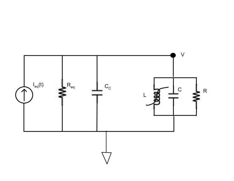
Figure 3: Equivalent circuit to Fig. 2. Note that $R_{eq}=2Z_{0}/(\omega_{0}C_{c}Z_{0})^{2}$ with $\omega_{0}=1/\sqrt{LC}$ and $I_{eq}=V_{s}/Z_{0}$. The voltage $V$ is then identical in the two circuits.

Note that the measurable quantity $V_{2}$ has disappeared from this circuit. But is easily recovered from the voltage $V$ via the linear circuit relationZmunpub

$$V_{2}={1\over 2}V_{s}+(i\omega_{0}C_{c}Z_{0})V$$ (1)

This is valid for $\omega_{0}C_{c}Z_{0}<<1$. Eq. (1) is understood to be in the frequency domain, with the “i” indicating that the contribution of $V$ to the signal $V_{2}$ is out of phase with that of the drive $V_{s}$.

We will take $V_{s}$ to be a classical ac variable with a simple sinusoidal time dependence:

$$V_{s}(t)=V_{s}\cos(\omega_{p}t)$$ (2)

We will assume that the nonlinear inductance is characterized by the small-signal energy storage formula

$$E_{L}={1\over 2}{\Phi^{2}\over L}+{1\over 4}{\Phi^{4}\over L_{4}}$$ (3)

$\Phi$ is the (formal) magnetic flux through this inductor, i.e., $\Phi(t)=\int^{t}V_{L}(t^{\prime})dt^{\prime}$. Other powers of $\Phi$ will generally appear in this energy, but our truncation will often be very accurate. This energy expression implies the non-linear inductive two-terminal response

$$I_{L}={\partial E_{L}\over\partial\Phi}={\Phi\over L}+{\Phi^{3}\over L_{4}}\ .$$ (4)

Using any standard circuit mechanics treatment (e.g., BKD ), the Hamiltonian of the circuit of Fig. 3 is then

$$H={1\over 2}{Q^{2}\over C^{\prime}}+\left({1\over 2}{\Phi^{2}\over L}+{1\over 4}{\Phi^{4}\over L_{4}}\right)+{V_{s}(t)\over Z_{0}}\Phi$$ (5)

Here $C^{\prime}=C+C_{c}$. The classical equation of motion for $\Phi$ will also have a “friction” term going like

$$-{{\dot{\Phi}}\over R^{\prime}},\,\,\,\,\,\,{1\over R^{\prime}}={1\over R_{eq}}+{1\over R},\,\,\,\,\,R_{eq}={2Z_{0}\over(\omega_{0}C_{c}Z_{0})^{2}}$$ (6)

Note that the voltage $V$ of interest here is related to our canonical momentum via the two-terminal relation for the linear capacitive element:

$$V={Q\over C^{\prime}}\ .$$ (7)

II.2 Quantum treatment

We go over now to a quantum treatment of the circuit. This will give $Q$, and therefore $V$ and $V_{2}$, the status of a quantum operators. We will assume that the experiment consists of a sequence of weak measurements of $V_{2}$, so that we will extract the expectation value $\langle V_{2}\rangle$, and that the system is not otherwise disturbed by the measurement. The standard quantum commutation relations are

$$[\Phi,Q]=i\hbar$$ (8)

Introducing bosonic creation and annihilation operators, we have

$$Q=-i\sqrt{\hbar\over 2}\left({C^{\prime}\over L}\right)^{1\over 4}(a_{\rm Sch}-a_{\rm Sch}^{\dagger}),$$ (9)

and similarly for $\Phi$. Here the subscript on the operator $a$ stands for “Schrodinger picture,” as we will soon do most of our calculations in an interaction picture.

Using this operator expression for $Q$ in Eqs. (9), we can get a quantum expression for the observable $V_{2}$. Going to the time domain:

$$\langle V_{2}\rangle={1\over 2}V_{s}\cos\omega_{p}t+{\omega_{0}C_{c}Z_{0}\over C^{\prime}}({\rm Re}\langle a\rangle\cos\omega_{p}t+{\rm Im}\langle a\rangle\sin\omega_{p}t)$$ (10)

The Hamiltonian operator describing the coherent part of the system evolution becomes

$$H_{S}=\hbar\omega_{0}a_{\rm Sch}^{\dagger}a_{\rm Sch}+{\hbar\chi\over 6}(a_{\rm Sch}+a_{\rm Sch}^{\dagger})^{4}+2\hbar\epsilon\cos(\omega_{p}t)(a_{\rm Sch}+a_{\rm Sch}^{\dagger})$$ (11)

We now go to an interaction picture ($a=e^{-i\omega_{p}t}a_{\rm Sch}$, etc.), and perform a rotating-wave approximation, obtaining

$$H=\hbar\Delta a^{\dagger}a+\hbar\chi(a^{\dagger})^{2}a^{2}+\hbar\epsilon(a+a^{\dagger})$$ (12)

Here the detuning $\Delta$ is $\Delta=\omega_{0}-\omega_{p}$, and we introduce scaled parameters, all with units sec^-1:

$$\omega_{0}={1\over\sqrt{LC^{\prime}}},\,\,\,\chi={3\hbar\over 8}{L\over C^{\prime}L_{4}},\,\,\,\,\epsilon={1\over\sqrt{8\hbar}}\left({L\over C^{\prime}}\right)^{1\over 4}{V_{s}\over Z_{0}}.$$ (13)

The lossy parts of our circuit are accounted for using the usual bosonic bath description; making the standard Born-Markov approximations Leggett ; BKD , and assuming the bath to be at zero temperature, the system dynamics is described by the Lindblad master equation:

$${d\rho\over dt}=-{i\over\hbar}[H,\rho]+{\gamma\over 2}(2a\rho a^{\dagger}-a^{\dagger}a\rho-\rho a^{\dagger}a)$$ (14)

with

$$\gamma={1\over R^{\prime}C^{\prime}}.$$ (15)

In this rescaled form, our model is identical to one employed recently in nanomechanics by Babourina-Brooks, Doherty, and MilburnBBDM . In fact, its essential features were already calculated thirty years ago by Drummond and WallsDW . In this paper, we will explore this rich solution and provide physical insights into some of its many interesting regimes.

II.3 spectroscopy

We will model the “spectroscopy” experiment as done in SQUIDless and in many other recent studies of superconducting qubit systems. Spectroscopy is measured as the magnitude of the ac output voltage signal at the same frequency as the input. For the model above, this will be proportional to the expectation value of $a$ in steady state:

$$\langle a\rangle={\rm Tr}(a\rho_{0})$$ (16)

Where $\rho_{0}$ is the steady state response:

$${d\rho_{0}\over dt}=0$$ (17)

We can write the Lindblad master equation in the form

$${d\rho\over dt}=S[\rho]$$ (18)

where $S$ is a linear superoperator, generating a TCP (trace preserving completely positive) map $e^{St}$. The resulting equation for the steady state,

$$S[\rho_{0}]=0$$ (19)

states that $\rho_{0}$ is obtained as the zero eigenvector of the linear non-Hermitian (super)operator $S$. It is this point of view that is employed in the numerical studies that we present below.

But numerics are only necessary for developing physical explanations, since the spectroscopy calculation itself, remarkably, has a closed form solution. Quoting Eq. (5.17) of DW :

$$\langle a\rangle={\epsilon\over\Delta-i\gamma/2}{\,{}_{0}F_{2}\left({\Delta+\chi-i\gamma/2\over\chi},{\Delta+i\gamma/2\over\chi},{2\epsilon^{2}\over\chi^{2}}\right)\over\,{}_{0}F_{2}\left({\Delta-i\gamma/2\over\chi},{\Delta+i\gamma/2\over\chi},{2\epsilon^{2}\over\chi^{2}}\right)}\ .$$ (20)

Here $\,{}_{0}F_{2}$ is a standard hypergeometric function.

III Results

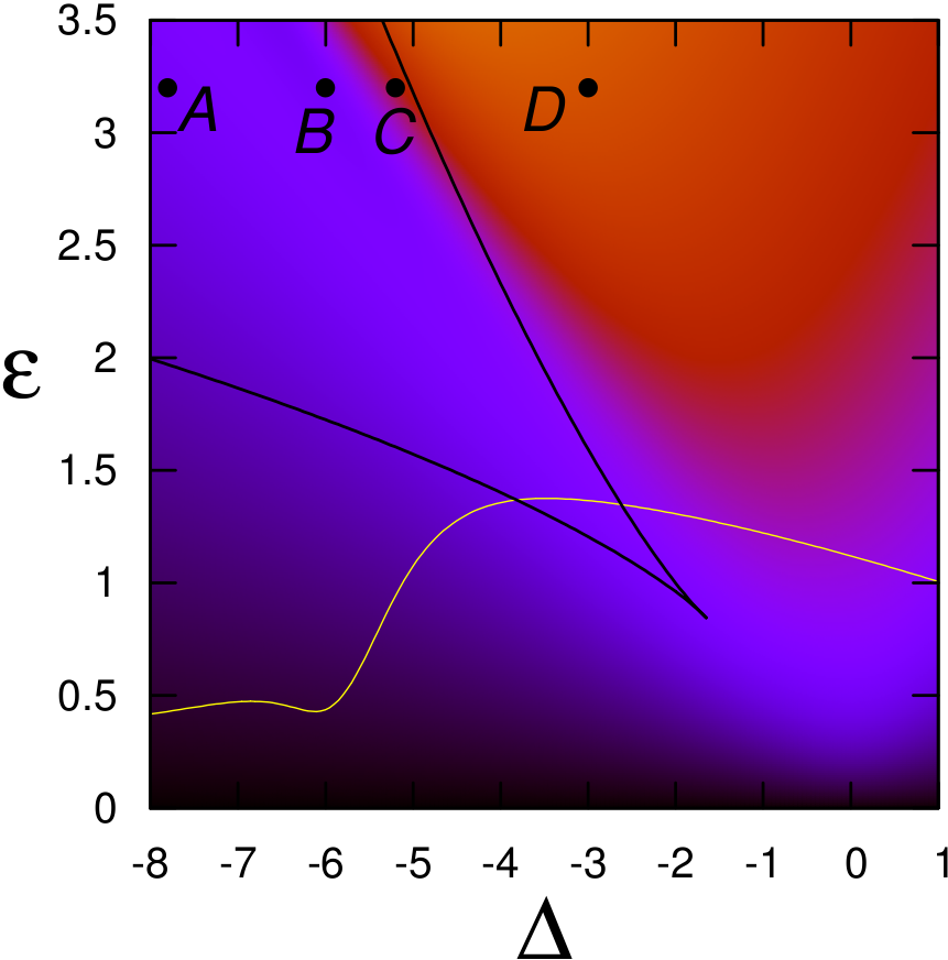
(a) $\gamma=2$

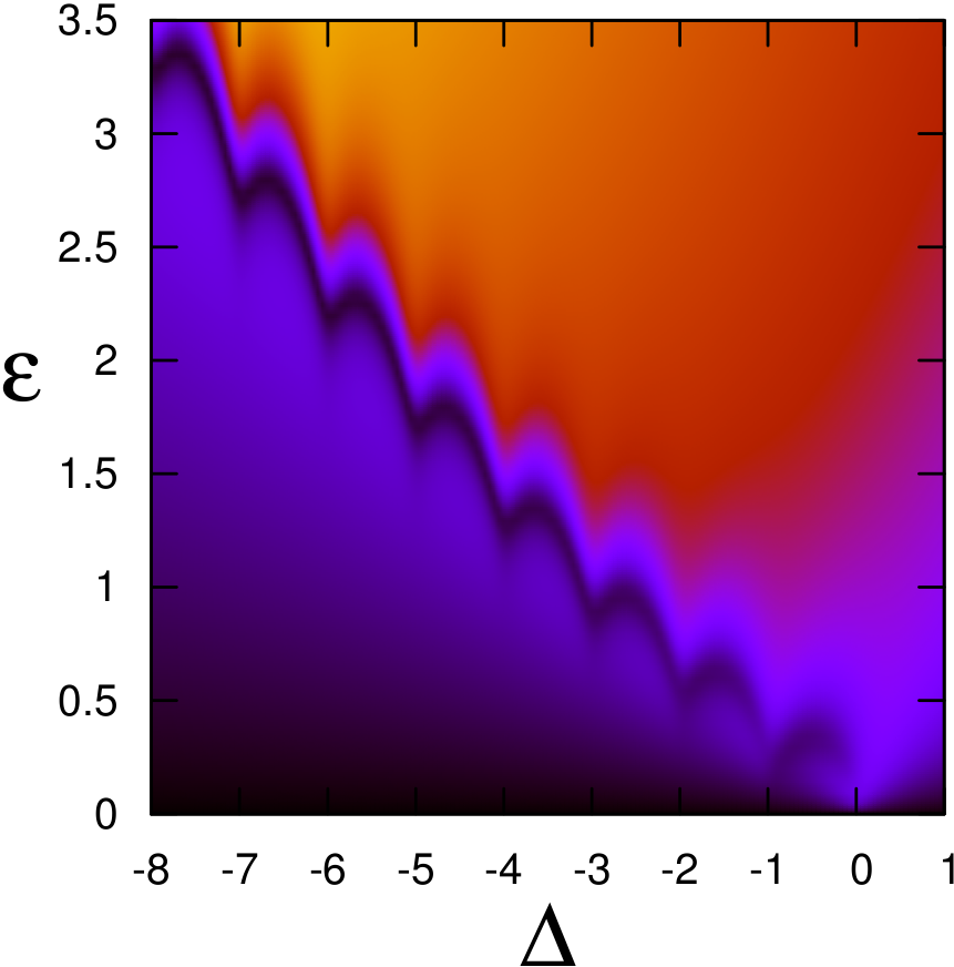
(b) $\gamma=0.3$

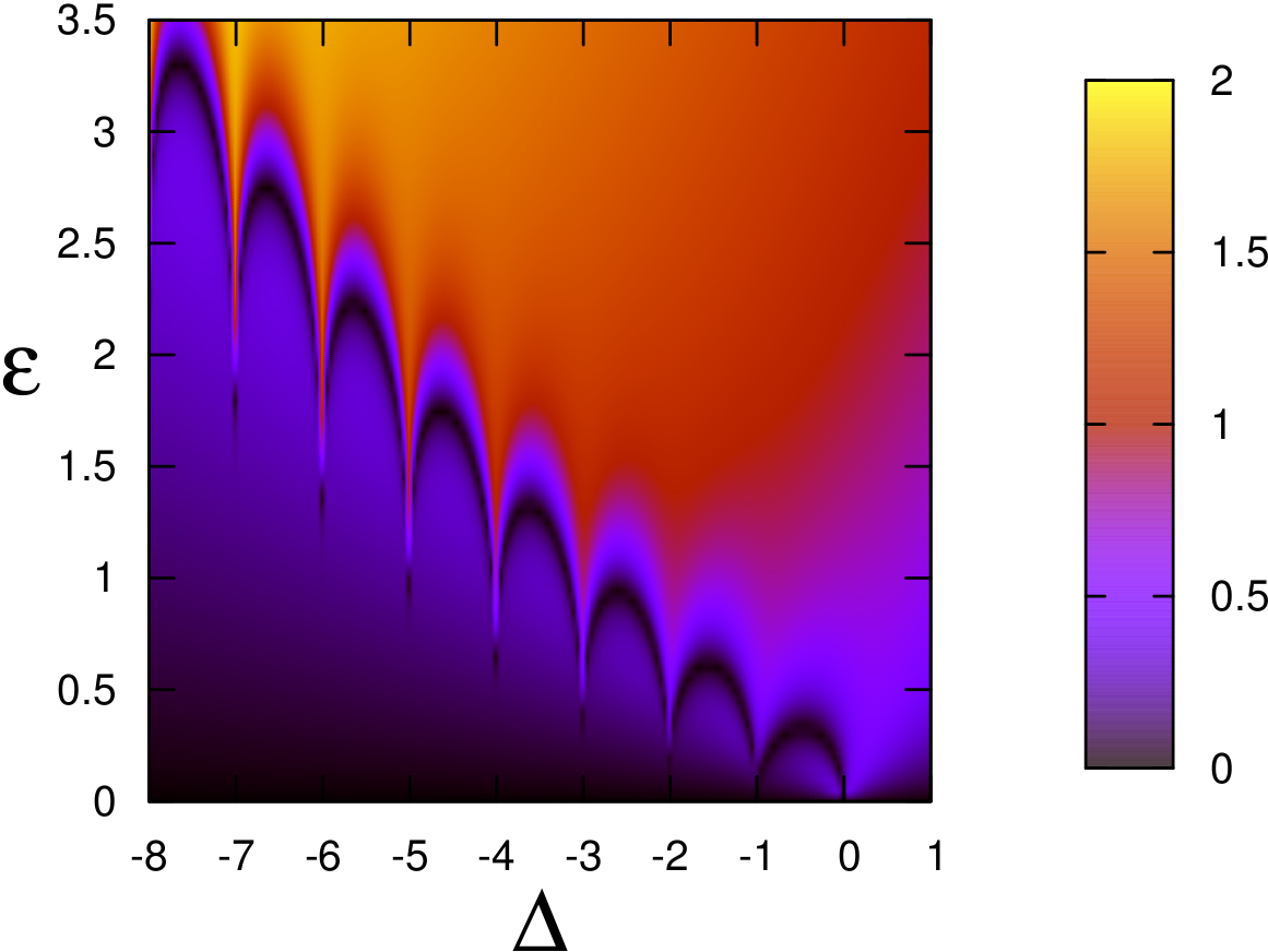
(c) $\gamma=0.01$

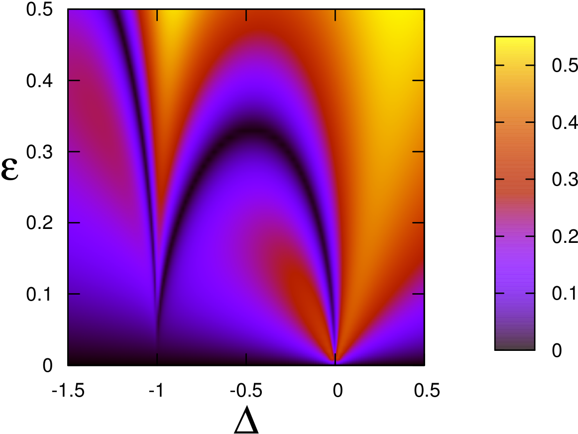
(d) $\gamma=0.01$

Figure 4: Response amplitude $|\langle a\rangle|$ as a function of detuning $\Delta$ and excitation amplitude $\epsilon$, all for anharmonicity parameter $\chi=1$. (a) Moderately high damping ($\gamma=2$). Red line: scan across the response at $\epsilon=3.2$. Points A, B, C, and D along this scan path are examined further in Fig. 5. The trough at point $B$ is easily visible in the line scan. Dark lines show the boundary of the metastable points bifur for the classical Duffing oscillation with these same parameters. (b) Response for moderate damping $\gamma=0.3$. Trough has become more prominent but is now scalloped, indicating the development of discrete quantum resonances. (c) Response for low damping $\gamma=0.01$. Quantum resonant structure becomes very prominent. (d) A closer view of the first resonant structure in the low damping case $\gamma=0.01$.

For three different damping parameters $\gamma$, Fig. 4 shows $|\langle a\rangle|$, which is proportional to the magnitude of the transmitted voltage in a spectroscopy experiment. The plots are shown as a function of $\Delta$, the detuning away from the harmonic resonance frequency, and $\epsilon$, the drive intensity. These quantities are normalized to the anharmonicity parameter $\chi$ (i.e., $\chi=1$ in Eq. (12)). The three panels show three different settings of the damping parameter (again, relative to $\chi$). For the largest $\gamma$ shown ($\gamma=2$ in part (a)) the response is in some sense classical; no structure involving transitions between individual quantum mechanical levels is present at any excitation level. As we will discuss, though, there are many aspects of this result that are not classical in any naive sense.

The principal feature of Fig. 4(a) at moderate excitation levels ($\epsilon\gtrsim 1$) is a fairly abrupt upward step in the response, with a brief dip in between. This dip or trough has been noted previouslyDW ; TroughExpt ; TroughTheory , and is prominently seen in recent experiments; we will discuss its origin shortly. As $\gamma$ is decreased (Fig. 4(b)), this trough develops ripples that are synchronized with the quantum transitions in the anharmonic ladder of states. At very small $\gamma$ (Fig. 4(c)) these ripples resolve themselves into spectroscopic resonant peaks, which merge into the “high” continuum at large $\epsilon$. As we will discuss later, it is only in this third setting that it is meaningful to say that the anharmonic resonator behaves as a qubit, for the most part only at small excitation levels $\epsilon\lesssim\chi$ and near zero detuning $|\Delta|\lesssim\chi$.

IV Results: high damping regime

The true classical behavior would be quite different from what is seen in Fig. 4(a), as was noted already in DW . Inside the two lines shown in Fig. 4(b), these are two classical steady state solutions – the dynamics bifurcates at the meeting of these two lines, and is hysteretic above the bifurcation. A quantum treatment, even one with large loss, cannot show this bifurcation, although the quantum solution is in fact very close to the classical solution in the “low” region beneath the lower bifurcation line, and in the “high” region above the upper bifurcationDW . Qualitatively, this difference can be ascribed to the possibility of transitions between the two classical steady states; mathematically, it arises because the superoperator $S[\rho]$ has a unique zero eigenvalue. Classical hysteretic behavior can be and is recovered in a quantum treatment of the transient behavior, as studied recently in metastab .

Collapse of hysteresis due to quantum effects is actually well known FreedmanSarachik . Special to the anharmonic resonator system, however, is the robust trough easily seen in Fig. 4(a). As originally noted in DW , the trough can be reasonably explained by the observation that the classical “high” and “low” states have almost opposite phases, since the first is essentially a resonant response, while the second is non-resonant.

In the simplest view of the trough, the state intermittently switches back and forth between the high and low Gaussian state. While this gives a rough description of the situation at point $B$ in Fig. 4(a), the state there is in fact not purely a mixture of a low-amplitude with a high-amplitude Gaussian state. We explore this transition by examining the Wigner function $W$ of the steady state $\rho_{0}$ as we pass through the “trough” by varying the detuning $\Delta$. We use the standard formulaWigner

$$W(\alpha) = {\rm Tr}\left(D(-\alpha)\rho_{0}D(\alpha)\Pi\right)$$

$$D(\alpha) = \exp\left(\alpha a^{\dagger}-\alpha^{*}a\right),\,\,\,\Pi=\sum_{n=0}^{\infty}(-1)^{n}|n\rangle\langle n|$$ (21)

with complex displacement $\alpha$. The simplest is the Wigner function at the “low response” point $A$ (Fig. 5(a)). To the eye, this state is nearly a coherent state slightly displaced (i.e., with substantially less than one photon of excitation). In fact, the state has some excess noise (i.e., has a somewhat broader Wigner function than a coherent state), which can be measured by the von Neumann entropy $S_{\rm vN}(\rho)=-{\rm Tr}\rho\log\rho$. At point $A$, $S_{\rm vN}(\rho_{0})=0.03$ bits.

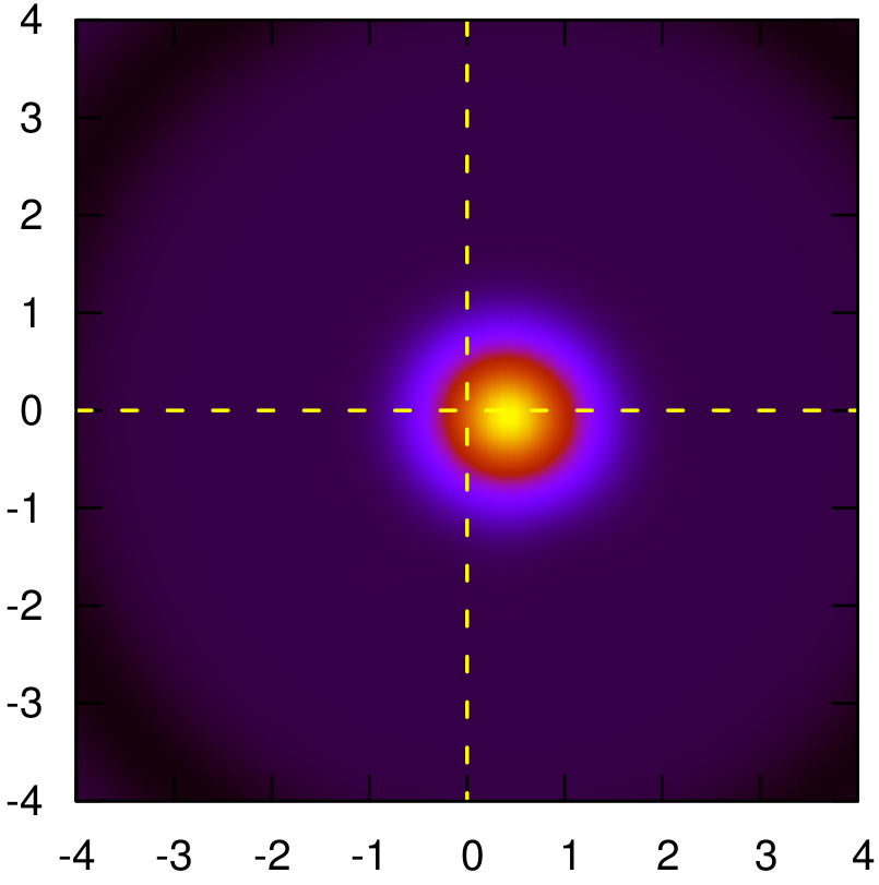
(a) Point $A$, $\Delta=-7.8$

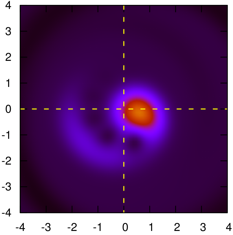
(b) Point $B$, $\Delta=-6.0$

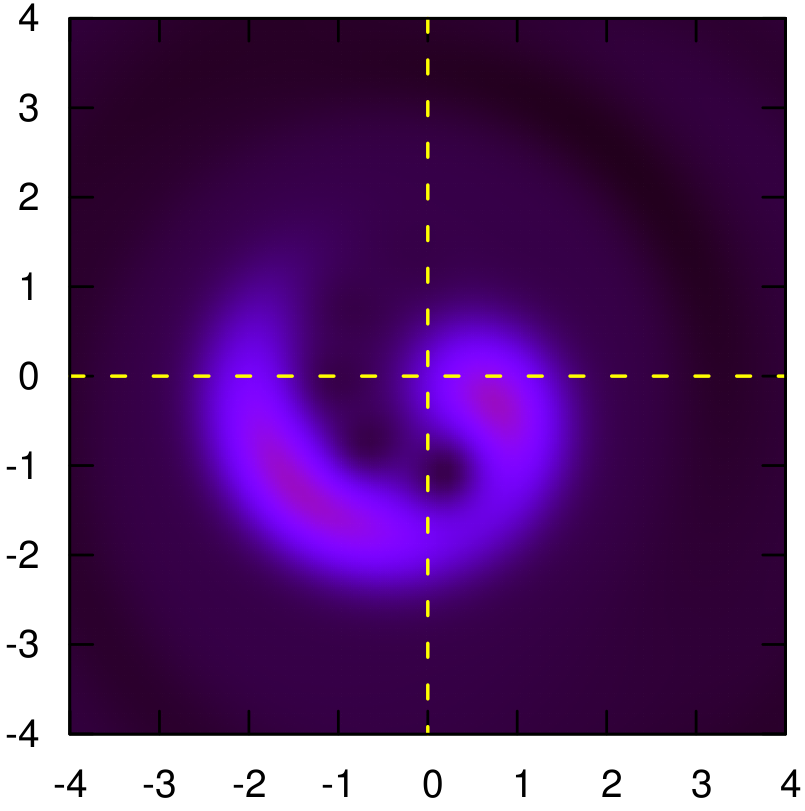
(c) Point $C$, $\Delta=-5.2$

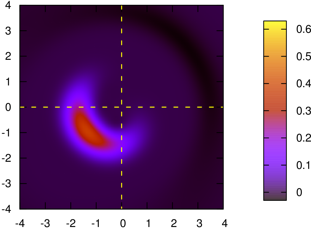
(d) Point $D$$,\Delta=-3.0$

Figure 5: Wigner functions for four points shown in Fig. 4.

The Wigner function at the “high response” point $D$ departs further from the simple classical view. This Wigner function (Fig. 5(d)) of course has a larger $|\langle\alpha\rangle|$ than in point $A$, but it is much farther from a coherent state. Despite its appearance, it is not number squeezed (the radial width is not smaller than a coherent state). It is perhaps better described as a coherent state with significant excess phase noise. The entropy of this state is $S_{\rm vN}=0.85$ bits.

The Wigner function in the transition region deserves considerable discussion. We will focus in detail on point $C$. The classical view that the state is a mixture of two classical responses is not entirely incorrect. But it fails to capture many of the aspects of the actual response. The system clearly spends appreciable time at phases intermediate between the high and low response, with $\bar{n}=2.56$, so it should not be viewed as quickly switching between the two. The state has high entropy, as a classical mixed state would, but its precise value ($S_{\rm vN}=1.74$) gives us more information about the nature of the state, as we explain now.

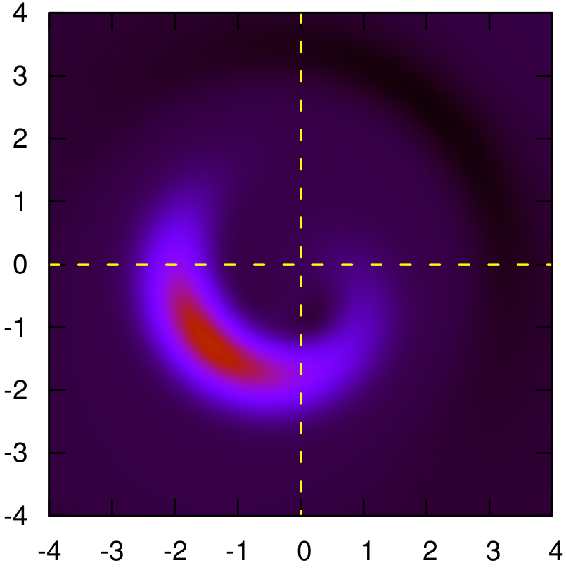
(a) $\rho_{-}$

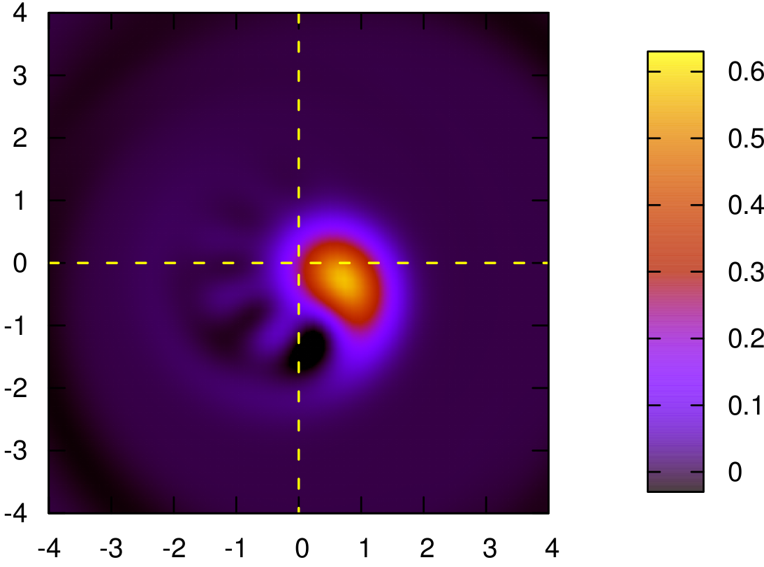
(b) $\rho_{+}$

Figure 6: Wigner functions of the extremal metastable responses at point $C$ ($\Delta=-5.2$) in the response diagram, showing that the picture that the Wigner function of the response (Fig. 5(c)) involves two possible metastable states is approximately, but not precisely, correct. Color scale is the same as in Fig. 5.

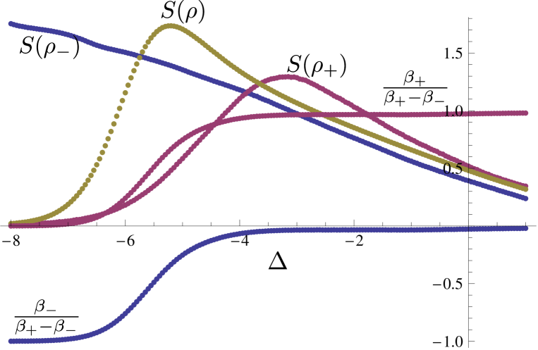
Figure 7: von Neumann entropies for the steady state $\rho$ and the extremal metastable states $\rho_{+}$ and $\rho_{-}$, as a function of $\Delta$ for $\epsilon=3.2$. Also shown are the coefficients $\beta_{\pm}$, suitably normalized, in Eq. (23).

The mixing picture is illuminated by a computation which pulls out a version of the two “classical response” states from the full state of Fig. 5(c); this is shown in Fig. 6. A vestige of the bistability of the classical response is clearly reflected in the eigenstructure of the superoperator $S$ at the operating point $C$. The second smallest eigenvalue if $S$ is at $\lambda_{1}=-0.215$, while the third eigenvalue is at $\lambda_{2}=-2.204$. It is the presence of two very nearby low lying eigenvalues $\lambda_{0,1}$, with a large separation from the rest of the spectrum, is a reflection of the classical bistability. It is straightforward to calculate this second eigenvector $|1)$ a.k.a. $\delta\rho_{1}$: $S|1)=\lambda_{1}|1)$. We use the notation $\delta\rho$ as a reminder that while this eigen-matrix is Hermitian (because it is associated with a real eigenvalue, rather than with a complex-conjugate pairsupopI ), it is traceless. But the important object we can construct from $\delta\rho_{1}$ is

$$\rho_{0}+\beta\delta\rho_{1}.$$ (22)

For real $\beta$. There will be a range of $\beta$s, including $\beta=0$, for which the operator will be positive semidefinite. We find that the two extremal operators, the one with the smallest possible $\beta=\beta_{-}<0$ and the largest possible $\beta=\beta_{+}$¿0, are the ones corresponding to the two classical solutions. Fig. 6 shows the Wigner functions of these two density operators,

$$\rho_{\pm}=\rho_{0}+\beta_{\pm}\delta\rho_{1}$$ (23)

We can see that this does a reasonably good job of separating the response into a high-amplitude and a low-amplitude part. This is also confirmed by the calculation of the von Neumann entropy of the range of states Eq. (22) (Fig. 7). The two extremal states $\rho_{\pm}$ are those of the lowest entropy. Classically, the states in the interior of this range (including $\rho_{0}$) should have an excess entropy above the weighted average of the extremal states (see Fig. 7) equal to the ordinary binary entropy of mixing $H(x)\equiv-x\log x-(1-x)\log(1-x)$. In fact Fig. 7 differs from this classical situation in two respects: 1) The maximal entropy of mixing is not 1 bit, but about 0.74 bits. 2) The excess entropy is nearly proportional to $H(x)$, but not exactly so, reflecting a quantum effect, the noncommutivity of the extremal states $[\rho_{-},\rho_{+}]\neq 0$.

V Results: Low damping regime

We now turn our attention to the lightly damped regime (by which we will mean $\gamma\lesssim\chi$). We expect that it is in this regime that our anharmonic oscillator “is” or “behaves like” a qubit. We will explore the light that our response calculation can shed on the question of when such an oscillator is or is not a qubit.

The outstanding qualitative feature of the response as $\gamma$ is lowered (as in the series in Fig. 4) is that stalactites form, descend, and sharpen from the bottom of the high-response continuum. The continuum itself, at least in the vicinity of the classical upper bifurcation line of Fig. 4(a), is not much affected by the lowering of $\gamma$. The trough remains an important feature, becoming first slightly, and then strongly, scalloped, finally breaking up into segments between one stalactite and the next.

Given that the quantum energy levels $\omega_{n}$ for the quartic oscillator obey to good approximation the simple rule

$$\omega_{n+1}-\omega_{n}=\omega_{0}+n\chi,$$ (24)

it is natural to associate the resonant structure at zero detuning with the “qubit” $0\rightarrow 1$ transition, the structure at detuning $\Delta=-\chi$ with the $1\rightarrow 2$ transition, that at $\Delta=-2\chi$ with the $2\rightarrow 3$ transition, and so forth. We might be tempted to guess that excitation detuning $\Delta=-n\chi$, the system is acting like a qubit involving the levels $|n\rangle$ and $|n+1\rangle$. As we will seen this is most definitely not the case, except for $n=0$. A detailed inspection of the $n=0$ “stalactite” shows that its structure is quite distinct from that of all the others. In fact, the excitation structures at higher $n$ are indicative of interesting multi-level behavior, as we will see.

V.1 A perturbation theory

We will do a perturbation analysis in $\epsilon$ to elucidate the nature of the resonant structures that appear as the excitation level is increased. While much can be learned simply by Taylor expansion of the exact expression for $|\langle a\rangle|$, much more is revealed by developing perturbative expressions for the eigenoperator of the superoperator $S$.

To develop this, we first record an explicit matrix form for this superoperator:

$$S_{kl,ij}\rho_{ij} = \{-i[\Delta(k-l)+\chi[k(k-1)-l(l-1)]]\delta_{ki}\delta_{lj}$$ (25)

$$-i\epsilon(\sqrt{k+1}\delta_{k,i-1}\delta_{lj}+\sqrt{k}\delta_{k,i+1}\delta_{lj}-\sqrt{l}\delta_{ki}\delta_{j+1,l}-\sqrt{l+1}\delta_{ki}\delta_{j-1,l})$$

$$+{\gamma\over 2}[2\sqrt{(k+1)(l+1)}\delta_{k+1,i}\delta_{l+1,j}-(k+l)\delta_{ki}\delta_{lj}]\}\rho_{ij}$$

S is sparse, but of course it is not, as a matrix, Hermitian. We analyze the steady state response by a perturbation approach. we can separate $S$ thus:

$$S=S_{0}+\epsilon V$$ (26)

$S_{0}$ can be analytically diagonalized – it has a “bidiagonal” form as a matrix. It is convenient to index its eigensolutions by two integers $n$ and $q$. Since $S_{0}$ is non-Hermitian, it is necessary to distinguish its right from its left eigenvectors,

$$S_{0}|nq_{R})=\lambda_{nq}|nq_{R})$$ (27)

$$(nq_{L}|S_{0}=(nq_{L}|\lambda_{nq}$$ (28)

Recall that the left eigenvectors are not the adjoint of the right eigenvectors, but the matrix formed by the left eigenvectors is the inverse of the matrix of right eigenvectors. The physical steady state response to zeroth order in $\epsilon$ is the eigenvector $|00_{R})$.

$S_{0}$ has both real and complex eigenvalues, for both of which ${\rm Re}\lambda_{nq}<0$ for $\epsilon\neq 0$ (except for $\lambda_{00}$ which is always equal to zero). It is straightforward to confirm the following: All the complex eigenvalues of $S_{0}$ may be written

$$\lambda_{nq}=-\left(q+{n\over 2}\right)\gamma-ni\Delta-n(n-1+2q)i\chi$$ (29)

with integers $q\geq 0$, $n>0$. The right eigenvectors $|nq)$ (a.k.a. $\rho_{nq}$, see Ref. Caves ) are operators on the Hilbert space with matrix elements

$$\langle s|\rho_{nq}|t\rangle=\delta_{s,t+n}{\left(-1-2n{i\chi\over\gamma}\right)^{t}\over(q-t)!\sqrt{s!t!}}\ .$$ (30)

Each has a complex conjugate partner $\lambda_{{\bar{n}}q}=\lambda^{*}_{nq}$, $\rho_{{\bar{n}}q}=\rho^{\dagger}_{nq}$. The real eigenvalues and right eigenvectors are given by the same formulas with $n=0$. We do not record the left eigenvectors $(nq|$ here, but they are as straightforward to write down as the right eigenvectors.

The right eigenvector $|00_{R}^{\rm full})$ of the full superoperator can be conveniently developed using Brillouin-Wigner perturbation theoryBaym . Going over to a schematic single-integer indexing of the eigenstates:

$$|0_{R}^{\rm full})=|0_{R})+\epsilon\sum_{k>0}{|k_{R})(k_{L}|V|0_{R})\over E_{0}-\lambda_{k}}+\epsilon^{2}\sum_{k>0}\sum_{j>0}{|k_{R})(k_{L}|V|j_{R})(j_{L}|V|0_{R})\over(E_{0}-\lambda_{k})(E_{0}-\lambda_{j})}+...$$ (31)

The Brillouin-Wigner formula is frequently not used because the exact eigenvalue $E_{0}$ is unknown. But in this application, of course, $E_{0}=0$ exactly; so this series is actually very useful, and its first few terms are readily calculated.

V.2 Characteristics of the resonant response

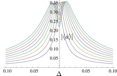
Figure 8: Response $|\langle a\rangle|$ for low damping, showing the emergence of the line at zero detuning. Here $\gamma=.01$, $\chi=1$, and from bottom to top, $\epsilon=.002,.003,.004,.005,.006,.007,.008,.009,.01$. At the low excitation level the response is Lorentzian and corresponds exactly to the linear response of a qubit; the higher lying levels play no role in the response. The hole in the center of the line at the highest $\epsilon$ is also a qubit effect, showing the incipient saturation of the qubit response. The asymmetry of the line around zero detuning occurs because of participation of higher levels, and would be the first indication that the system is not a qubit as the excitation level is raised.

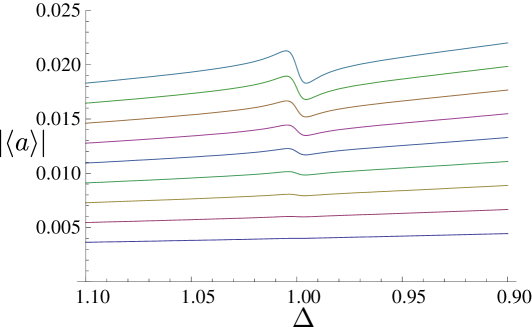
Figure 9: Response $|\langle a\rangle|$ for low damping, showing the emergence of the line at detuning $\Delta=-\chi$. Here $\gamma=.01$, $\chi=1$, and, from bottom to top, $\epsilon=.004,.006,.008,.010,.012,.014,.016,.018,.02$. The structure emerges as a Fano resonance out of the continuum of the far off resonant response at zero detuning.

Using this perturbation theory, we can write out in matrix representation (in the number basis) the steady state response in orders of $\epsilon$:

$$\rho_{0}^{\rm approx}\approx\left(\begin{array}[]{cccc}1-O(\epsilon^{2})&\cdot&\cdot&\cdot\\ \begin{array}[]{l}{2\epsilon\over-2\Delta+i\gamma}\,\,+\\ {8\epsilon^{3}(4\chi+2\Delta-i\gamma)\over(2\Delta-i\gamma)^{2}(2\chi+2\Delta-i\gamma)(2\Delta+i\gamma)}\end{array}&O(\epsilon^{2})&\cdot&\cdot\\ O(\epsilon^{2})&{-8\epsilon^{3}\over(2\Delta-i\gamma)(2\chi+2\Delta-i\gamma)(2\Delta+i\gamma)}&O(\epsilon^{4})&\cdot\\ O(\epsilon^{3})&O(\epsilon^{4})&O(\epsilon^{5})&O(\epsilon^{6})\end{array}\right)\ .$$ (32)

The matrix is Hermitian, and we have omitted the entries above the diagonal. We have only shown in detail the matrix elements $\langle 1|\rho_{0}^{\rm approx}|0\rangle$ and $\langle 2|\rho_{0}^{\rm approx}|1\rangle$, since these are the only ones that contribute to the the observable $\langle a\rangle$; but, as we note, there are many non-zero unobservable components to this steady-state density operator.

We also note the expression for the total response that can be extracted either from this or via a Taylor expansion of Eq. (20):

$$\langle a\rangle={2\epsilon\over 2\Delta-i\gamma}-{32\chi\epsilon^{3}\over(2\Delta-i\gamma)^{2}(2\chi+2\Delta-i\gamma)(2\Delta+i\gamma)}+O(\epsilon^{5})\ .$$ (33)

First we turn our attention to the resonant structure near zero detuning $\Delta=0$, shown in Fig. 8. For small $\epsilon$, as the expression in Eq. (33) shows, the response is a simple Lorentzian, just as expected for a driven two-level system. In this regime, the oscillator behaves exactly like a qubit, which would, in the transient regime, respond as any two level system would to Rabi excitation or to Ramsey or spin-echo protocols. When $\epsilon$ become of order $\gamma$, new structure appears. The top of the Lorentzian peak becomes flat and then exhibits a growing hole. One might say that at this point the higher levels of the oscillator are participating, but in fact this is very close to the behavior shown by a two level system in the regime of spectroscopy probed at high power. As recently shown in BishChow , saturation of the two level system causes just this same evolution into a double peaked structure. But some features of this regime are indicative of the participation of higher levels. The development of line asymmetry is definitely ascribed to higher levels; this asymmetry diminishes in the limit of large $\chi$.

Mathematically, we see from Eq. (32) that these new structures in the zero-detuning line all arise from the $O(\epsilon^{3})$ contributions. Note that only odd orders contribute observably to $\langle a\rangle$, consistent with the fact that the response should be an odd function of $\epsilon$. The $O(\epsilon^{3})$ response involves all of the first four levels, so in some sense the line at this excitation level is indicative of four-level system response. But it is not clear that one need adopt this point of view, since the 0-3 matrix element of the steady state response is not visible to our problem, although one could construct a more complex observable that is sensitive to it.

We next turn to an examination of the resonant structure near $\Delta=-\chi$, at the “$1\rightarrow 2$ transition”. The linear response has no resonant structure at this detuning, but the $\epsilon^{3}$ part of the response is resonant here. But the linear response has a uniform far off resonant background at this detuning, and resonance emerges our of this background (see Fig. 9). Thus, the behavior here is very different in detail from the no-detuning line, although mathematically, they arise from two different poles of the same matrix elements in Eq. (32).

Furthermore, it is easy to show that because of interference of the resonant response with the background, the line that emerges in Fig. 9 has a Fano line shapeFanoline

$$|\langle a\rangle|\sim|\langle a\rangle|_{background}+C{(x-q)^{2}\over x^{2}+1}$$ (34)

with suitably normalized frequency $x$. The Fano parameter $q$ is easy to calculate:

$$q={-2\chi\over\sqrt{2\chi^{2}+\gamma^{2}}-\gamma}$$ (35)

Since we are in a regime where $\gamma<<\chi$, this Fano parameter is close to $-1$. $q=-1$ is among the most asymmetrical of the Fano line shapes Fano61 , in striking contrast to the initial symmetry of the distorted zero-detuning line. This Fano line exhibits a trough on the high-frequency side of the line. This is the beginning of the trough that forms a scallop from one “stalactite” to the next, and so it is the structure that has continuously evolved from the semiclassical trough that occurs at high damping. It is curious that the classical interference arising from intermittency at high damping evolves continuously into a Fano destructive interference, which we think of as entirely quantum mechanical.

We will say much less about the resonant structures that arise at higher detuning, except to make a couple of observations: All higher lines emerge in a similar way to the $\Delta=-\chi$ line, with a Fano line shape with the same asymmetry (so, evidently, a similar $q$, which we have not calculated). Each emerges first at successively higher order in the response; so, the resonant line at $\Delta=-n\chi$ arises first at order $O(\epsilon^{2n+1})$. The calculation shows that the first appearance of the line from the background (as measured by the first appearance of a zero slope near the resonance frequency) occurs at an excitation level that goes like

$$\epsilon_{onset}=f(n)\chi^{1-{1\over n}}\gamma^{1\over n},$$ (36)

with some increasing function $f(n)$. We note that the dominant background is always the off resonant response of the zero-detuning line, rather than the background of any nearer by lines, no matter how large the value of $n$. So, from Eq. (36) we see that it is only the $n=0$ and $n=1$ lines that first show nonlinear structure at $\epsilon\sim\gamma$; structures at all higher detunings occur only at higher power (e.g., for $n=2$ the onset is at $\sqrt{\chi\gamma}$).

VI Discussion

It is clear that the present study is only a piece of the full picture in the theoretical modeling of the complete input-output relations for the excitation of qubit structures. The potential complexity of the decohering environment of these structures has barely been touched on here, and remains a frontier area of research. For actual applications, more of the essential further work will be in the time domain rather than the frequency domain; pulsed excitation of qubits, both for gate operations and for measurements, will definitely be the study of more extensive modeling as this experimental art develops further.

Still, the present simple study has revealed an intricate complex of phenomena. One example of a further study that it possible as a direct follow on to this work is the more detailed examination of the validity and limits of the rotating wave approximation. The simplicity of the mathematics here should permit a definite if limited answer to questions about this. These questions often do not have such a clear answer in a more general setting.

Another question raised by the present study concerns the emergence of classical bistability. As we have seen, the quantum theory says that there is a continuum of states (convex combinations of $\rho_{+}$ and $\rho_{-}$) that are metastable. Which two of them does the classical physics pick out? We have offered a conjecture here that the ones of locally minimum von Neumann entropy (which happen to be $\rho_{+}$ and $\rho_{-}$ themselves) are the classical states. Their low entropy is associated (albeit indirectly) with their high degree of localization of the Wigner function in the complex $\alpha$ plane. This in turn could make them candidates as “pointer states.” That is, it is possible that the right view of the quantum environment would make these states emerge naturally. Thus, even the most fundamental questions can have a profitable launching point from our simple model calculations.

Acknowledgments: The authors would like to thank Chad Rigetti for helpful discussions and comments on the text. JAS has been partially supported by the IARPA MQCO program under contract no. W911NF-10-1-0324.

References

- (1) Matthias Steffen, Shwetank Kumar, David DiVincenzo, George Keefe, Mark Ketchen, Mary Beth Rothwell, and Jim Rozen, “Readout for Phase Qubits without Josephson Junctions,” Appl. Phys. Lett. 96, 102506 (2010); arXiv:1001.1453.
- (2) M. D. Reed, L. DiCa rlo, B. R. Johnson, L. Sun, D. I. Schuster, L. Frunzio, R. J. Schoelkopf, “High Fidelity Readout in Circuit Quantum Electrodynamics Using the Jaynes-Cummings Nonlinearity,” arXiv:1004.4323.
- (3) Maxime Boissonneault, J. M. Gambetta, Alexandre Blais, “Improved Superconducting Qubit Readout by Qubit-Induced Nonlinearities,” Phys. Rev. Lett. 105, 100504 (2010) (arXiv:1005.0004); Lev S. Bishop, Eran Ginossar, S. M. Girvin, “Response of the Strongly-Driven Jaynes-Cummings Oscillator,” Phys. Rev. Lett. 105, 100505 (2010) (arXiv:1005.0377).
- (4) P. D. Drummond and D. F. Walls, “Quantum theory of optical bistability. I. Nonlinear polarisability model,” J. Phys. A 13, 725-741 (1980).
- (5) V. Peano, M. Thorwart, “Dynamical bistability in the driven circuit QED,” Europhys. Lett. 89 17008 (2010); arXiv:0903.2338.
- (6) J. Zmuidzinas, J. Gao, P. K. Day, and H. G. LeDuc, “Readout and isolation of frequency and dissipative perturbations in superconducting microresonators,” unpublished manuscript.
- (7) G. Burkard, R. H. Koch, and D. P. DiVincenzo, “Multi-level quantum description of decoherence in superconducting qubits,” Phys. Rev. B 69, 064503 (2004); arXiv:cond-mat/0308025.
- (8) A. J. Leggett, S. Chakravarty, A. T. Dorsey, M. P. A. Fisher, A. Garg, and W. Zwerger, “Dynamics of the dissipative two-state system,” Rev. Mod. Phys. 59, 1-85 (1987).
- (9) E Babourina-Brooks, A Doherty and G J Milburn, “Quantum noise in a nanomechanical Duffing resonator,” New J. Phys. 10, 105020 (2008); arXiv:0804.3618.
- (10) M. I. Dykman and M. A. Krivoglaz, “Fluctuations in nonlinear systems near bifurcations corresponding to the appearance of new stable states,” Physica 104A, 480-494 (1980).
- (11) Lingzhen Guo, Zhigang Zheng, and Xin-Qi Li, “Quantum Dynamics of Mesoscopic Driven Duffing Oscillators,” Europhys. Lett. 90, 10011 (2010); arXiv:0906.4981.
- (12) Jonathan R. Friedman, M. P. Sarachik, J. Tejada, R. Ziolo, “Macroscopic Measurement of Resonant Magnetization Tunneling in High-Spin Molecules,” Phys. Rev. Lett. 76, 3830-3833 (1996).
- (13) C. M. Caves, “Quantum Error Correction and Reversible Operations,” J. Superconductivity 12(6), 707-718 (1999); arXiv:quant-ph/9811082.
- (14) Max Hofheinz, H. Wang, M. Ansmann, Radoslaw C. Bialczak, Erik Lucero, M. Neeley, A. D. O’Connell, D. Sank, J. Wenner, John M. Martinis, and A. N. Cleland, “Synthesizing arbitrary quantum states in a superconducting resonator,” Nature 459, 546-549 (2009).
- (15) B. M. Terhal and D. P. DiVincenzo, “The problem of equilibration and the computation of correlation functions on a quantum computer,” Phys. Rev. A 61, 22301 (2000); arXiv:quant-ph/9810063.
- (16) G. Baym Lectures on Quantum Mechanics, (Benjamin, Reading, MA, 1969), p. 241.
- (17) Lev S. Bishop, J. M. Chow, Jens Koch, A. A. Houck, M. H. Devoret, E. Thuneberg, S. M. Girvin, R. J. Schoelkopf, “Nonlinear response of the vacuum Rabi resonance,” Nature Physics 5, 105-109 (2009); arXiv:0807.2882.
- (18) Kensuke Kobayashi, Hisashi Aikawa, Shingo Katsumoto, and Yasuhiro Iye, “Tuning of the Fano Effect through a Quantum Dot in an Aharonov-Bohm Interferometer,” Phys. Rev. Lett. 88, 256806 (2002); arXiv:cond-mat/0311497.
- (19) U. Fano, “Effects of Configuration Interaction on Intensitites and Phase Shifts,” Phys. Rev. 124 1866-1878 (1961).