Gravitational Fermion Production in Inflationary Cosmology

Abstract

We revisit the gravitational production of massive Dirac fermions in inflationary cosmology with a focus on clarifying the analytic computation of the particle number density in both the large and the small mass regimes. For the case in which the masses of the gravitationally produced fermions are small compared to the Hubble expansion rate at the end of inflation, we obtain a universal result for the number density that is nearly independent of the details of the inflationary model. The result is identical to the case of conformally coupled scalars up to an overall multiplicative factor of order unity for reasons other than just counting the fermionic degrees of freedom.

I Introduction

Gravitational particle production (as reviewed e.g in Birrell:1982ix ; DeWitt1975 ) and string production (see e.g. Lawrence:1995ct ; Gubser:2003vk ; Turok:2004gb ; Friess:2004zk ; Tolley:2005ak ; Cremonini:2006sx ; Das:2006dr ; Feng:2007qk ) are generic phenomena for quantum fields in a curved spacetime background and are analogs of particle creation in strong electric fields (see e.g. Schwinger1951 ; Brezin:1970xf ). In the case of Friedmann-Robertson-Walker (FRW) cosmology without inflation, it was found Audretsch1978 ; Mamaev1978 ; Mamaev1975 ; Parker1971 ; Parker1969 that the production of fermion and conformally coupled scalar fields near the radiation dominated (RD) universe singularity occurs when the particle masses $m$ are comparable to the Hubble expansion rate $H$, with a number density $n\sim m^{3}$ that dilutes as $a^{-3}$ due to expansion. The fractional relic density of these particles at the time of radiation-matter equality is $\Omega_{X}\sim(m_{X}/10^{9}\mbox{GeV})^{5/2}$ Kuzmin . Hence, the requirement of $\Omega_{X}<1$ puts an upper bound of $10^{9}\,\mbox{GeV}$ on the stable particle mass.

In contrast, in inflationary cosmology the previously unbounded rapid growth of $H$ as one moves backward in time towards the RD singularity is replaced by a nearly constant $H_{e}$ during the quasi-de Sitter (dS) era. In such cases, the possibility of superheavy dark matter in a wide range of masses including $m>H_{e}$ was emphasized in Chung:1998zb ; Kuzmin:1998kk . In fact, natural superheavy dark matter candidates existed in the context of string phenomenology before the gravitational production mechanism was appreciated Ellis:1990iu ; Benakli:1998ut . Furthermore, many extensions of the Standard Model also possess superheavy dark matter candidates (see e.g. Kusenko:1997si ; Han:1998pa ; Dvali:1999tq ; Hamaguchi:1999cv ; Coriano:2001mg ; Cheng:2002iz ; Shiu:2003ta ; Berezinsky:2008bg ; Kephart:2001ix ; Kephart:2006zd ), which can have interesting astrophysical implications (see e.g. Coriano:2001mg ; Barbot:2002gt ; Albuquerque:2003ei ; Taoso:2007qk ; Bovy:2008gh ; Albuquerque:2010bt ). In such contexts, analytic relic density formulae have been computed in the heavy and the light mass regimes for conformally coupled scalars Chung2003 ; Chung:2001cb ).

In this work, we turn our attention to the gravitational particle production of long-lived Dirac fermions in inflationary cosmology. Gravitational particle production of Dirac fermions has been studied numerically within the context of specific chaotic inflationary models Kuzmin:1998kk . Our purpose is to clarify the analytic computation and to derive a universal result for the light mass scenario that is nearly independent of the details of the inflationary model. Our result is identical up to an overall $O(1)$ multiplicative factor to that obtained for conformally coupled light scalar fields in Chung:2001cb , despite the fact that the Dirac structure naively imposes a different spectral (momentum scaling) property on the equations governing the particle production. In comparison to the conformally coupled scalar case, no special non-renormalizable coupling to gravity nor possibility of tadpole instabilities concern the fermionic scenario in the light mass limit because the fermion kinetic operator is conformally invariant and fermions cannot obtain a nonvanishing vacuum expectation value.

We also derive the particle production spectrum for the heavy mass scenario and find it to be identical to the result of Chung2003 (again up to an $O(1)$ multiplicative constant) despite a different momentum dependence of the starting point of the equations. As expected, the heavy mass number density falls off exponentially. In contrast with the light mass limit, this case is sensitive to the details of the transition out of the inflationary era. To emphasize the simplicity and the novel analytic arguments of the light mass scenario, we relegate the heavy mass results to an appendix.

It should be noted that the production of fermions in inflationary cosmology has been extensively considered during the recent past, but most analyses have focused on the non-gravitational interactions. For example, Garbrecht:2002pd ; PhysRevD.57.6003 ; Bassett:2001jg ; Peloso:2000hy ; GarciaBellido:2000dc ; PhysRevD.58.125013 ; Greene:1998nh ; Dolgov:1989us focused on both numerical and analytic analyses of fermion production during preheating. Chung:1999ve considered the production effects when the fermion mass passes through a zero during the quasi-dS phase. The effects of radiative corrections that modify the fermion dispersion relationship and its connection to particle production were considered in PhysRevD.73.064036 . Gravitino production has also been considered by many authors (see e.g. Maroto:1999ch ; Kallosh:1999jj ; Giudice:1999am ; Nilles:2001fg ; Nilles:2001ry ; Kawasaki:2006hm ). The main thrust of this paper differs in that it focuses on the minimal gravitational coupling and derives a simple bound analogous to Eq. (44) of Chung:2001cb . Indeed, our results will aid in future investigations similar to Berezinsky:2008bg which would benefit from a more accurate simple analytic estimate of the dark matter abundance.

The outline of this work is as follows. In Sec. 2, we discuss the intuition behind the general formalism for the gravitational production of massive Dirac fermions in curved spacetime. In Sec. 3, we discuss the generic features of the spectrum and derive the main result of this paper, which is that for a given mode with comoving wave number $k$, the Bogoliubov coefficient magnitude $|\beta_{k}|^{2}\sim O(1/2)$ if $H(\eta)>m$ when $k/a(\eta)\sim m$. We test this analytic result within a toy inflationary model in Sec. 4, and then discuss the dependence on reheating and the implications for the relic density in Sec. 5. Finally, in Sec. 6 we summarize our results and present our conclusions. Appendix A contains a collection of useful results for fermionic Bogoliubov transformation computations. Appendix B contains a complementary argument (which relies more on the spinorial picture of the fermions) for the universality of the Bogoliubov coefficient in the light mass region. Appendix C contains the particle density spectrum for the heavy mass limit.

II Fermion Particle Production: Background and Intuition

To compute the particle production of Dirac fermions in curved spacetime, we follow the standard procedure as outlined for example in Birrell:1982ix ; DeWitt1975 to calculate the Bogoliubov coefficient $\beta_{k}$ between the in-vacuum corresponding to the inflationary adiabatic vacuum and the out-vacuum corresponding to the adiabatic vacuum defined at post-inflationary times. The details of this formalism and our conventions are presented in Appendix A, with the expression for $\beta_{k}$ given in Eq. (81).

However, to obtain a better intuitive picture of the particle production mechanism, here we present general physical arguments regarding the expected features of the spectrum. We begin by considering a Dirac fermion field $\Psi$ described by

$$\mathcal{L}=i\bar{\Psi}\gamma^{\mu}\nabla_{\mu}\Psi-m\bar{\Psi}\Psi$$ (1)

minimally coupled to gravity. As the action $S=\int d^{4}x\sqrt{g}\mathcal{L}$ is conformally invariant in the $\{m\rightarrow 0,\,\hbar\rightarrow 0\}$ limit (with $\delta g_{\mu\nu}(x)=-2\sigma(x)g_{\mu\nu}(x)$), physical quantities are necessarily independent of the FRW scale factor $a$ to leading order in $\hbar$. Hence, the leading $\hbar$ order Bogoliubov coefficient $\beta_{k}$ is zero in the $ma/k\rightarrow 0$ limit, since it is the metric that drives the particle production (i.e., it plays the role of the electric field in the analogy of particle creation by strong electric fields). This implies that particle production can only occur in significant quantities for non-relativistic modes.

We next point out that the Dirac equation with a time-dependent mass term results in mixing between positive and negative frequency modes, similar to the case of the conformally coupled Klein-Gordon system with a time-dependent mass. To see this explicitly, consider the Dirac equation for the spinor mode functions $u_{A,B}$ that follows from Eq. (1):

$$i\partial_{\eta}\left(\begin{array}[]{c}u_{A}\\ u_{B}\end{array}\right)=\left(\begin{array}[]{cc}am&k\\ k&-am\end{array}\right)\left(\begin{array}[]{c}u_{A}\\ u_{B}\end{array}\right),$$ (2)

which is our Eq. (78) from Appendix A. Here $u_{A,B}$ span the complete solution space (they contain both approximate positive and negative frequency solutions in the adiabatic regime). Here we are working in conformal time, which is related to the comoving observer’s proper time via $dt\equiv a(\eta)d\eta$. From Eq. (2), we see that the rotation matrix that diagonalizes the right hand side is a function of the time-dependent quantity $am$. Hence, the Dirac equation as a function of time mixes approximate positive and negative frequency solutions leading to non-vanishing particle production.

To estimate the Bogoliubov coefficient, we can compute the effects of the time-dependent mixing matrix $\mathcal{U}\in O(2)$ as follows. We begin by inserting $1=\mathcal{U}^{T}\mathcal{U}$ into Eq. (2) to obtain

$$i\mathcal{U}\partial_{\eta}\left[\mathcal{U}^{T}\mathcal{U}\left(\begin{array}[]{c}u_{A}\\ u_{B}\end{array}\right)\right] = \mathcal{U}\left(\begin{array}[]{cc}am&k\\ k&-am\end{array}\right)\mathcal{U}^{T}\mathcal{U}\left(\begin{array}[]{c}u_{A}\\ u_{B}\end{array}\right)$$ (9)

$$\implies i\mathcal{U}\partial_{\eta}\mathcal{U}^{T}\left(\begin{array}[]{c}u_{A}^{\prime}\\ u_{B}^{\prime}\end{array}\right)+i\partial_{\eta}\left(\begin{array}[]{c}u_{A}^{\prime}\\ u_{B}^{\prime}\end{array}\right) = \left(\begin{array}[]{cc}\sqrt{k^{2}+m^{2}a^{2}}&0\\ 0&-\sqrt{k^{2}+m^{2}a^{2}}\end{array}\right)\left(\begin{array}[]{c}u_{A}^{\prime}\\ u_{B}^{\prime}\end{array}\right),$$ (18)

in which the primed basis is defined to be

$$\left(\begin{array}[]{c}u_{A}^{\prime}\\ u_{B}^{\prime}\end{array}\right)\equiv\mathcal{U}\left(\begin{array}[]{c}u_{A}\\ u_{B}\end{array}\right).$$ (19)

The Dirac equation is diagonal in the primed basis except for the appearance of the mixing term

$$\mathcal{U}\partial_{\eta}\mathcal{U}^{T}=\frac{a}{2}\left(\begin{array}[]{cc}0&\frac{mHk_{p}}{k_{p}^{2}+m^{2}}\\ -\frac{mHk_{p}}{k_{p}^{2}+m^{2}}&0\end{array}\right),$$ (20)

with $k_{p}\equiv k/a$. From this result, we see that during inflation the mixing term approximately vanishes for a fixed comoving wave number $k$ as $a\rightarrow 0$, while after inflation it is the largest when $H$ is the largest. Using this result, it is straightforward to show that the Bogoliubov coefficients due to mixing take the following form:

$$\beta_{k}^{\mbox{mix}}\sim\int dt\frac{mk_{p}}{k_{p}^{2}+m^{2}}He^{-2i\int dt\,\omega_{k}},$$ (21)

in which $\omega_{k}=\sqrt{k_{p}^{2}+m^{2}}$. One may still ask whether there are any other sources of positive and negative frequency mixing since the diagonal terms of Eq. (18) are time dependent, just as conformally coupled scalar fields contain $\omega^{2}=k^{2}+m^{2}a^{2}$ in their mode equations. The answer is no if the fermionic particles are defined as modes that exactly satisfy the condition

$$i\partial_{\eta}\left(\begin{array}[]{c}u_{A}^{\prime}\\ u_{B}^{\prime}\end{array}\right)=\left(\begin{array}[]{cc}\sqrt{k^{2}+m^{2}a^{2}}&0\\ 0&-\sqrt{k^{2}+m^{2}a^{2}}\end{array}\right)\left(\begin{array}[]{c}u_{A}^{\prime}\\ u_{B}^{\prime}\end{array}\right).$$ (22)

For example, the adiabatic vacuum positive frequency modes are defined to be

$$\left(\begin{array}[]{c}u_{A}^{\prime}\\ u_{B}^{\prime}\end{array}\right)\propto\left(\begin{array}[]{c}1\\ 0\end{array}\right)e^{-i\int dt\sqrt{\frac{k^{2}}{a^{2}}+m^{2}}}.$$ (23)

Eq. (23) corresponds to a zeroth order adiabatic vacuum in which the adiabaticity parameter $\epsilon_{A}$ is defined as

$$\epsilon_{A}\equiv\frac{mHk_{p}}{\left(k_{p}^{2}+m^{2}\right)^{3/2}},$$ (24)

in accordance with the usual conventions Birrell:1982ix ; Parker1969 ; Chung:1998zb ; Chung:2003wn . This parameter vanishes in the asymptotically far past (near when the in-vacuum is defined) and in the far future (near when the out-vacuum is defined). Eq. (23) coincides with

$$\left(\begin{array}[]{c}u_{A}\\ u_{B}\end{array}\right)\rightarrow\left(\begin{array}[]{c}\sqrt{\frac{\omega+am}{2\omega}}\\ \sqrt{\frac{\omega-am}{2\omega}}\end{array}\right)e^{-i\int^{\eta}d\eta^{\prime}\omega}$$ (25)

in the basis of Eq. (2).

To summarize, the zeroth adiabatic order vacuum Bogoliubov coefficient is approximately given by Eq. (21). We see that compared to the conformally coupled bosonic case (see e.g. Chung2003 ), the long wavelength fermionic particle production is suppressed due to the appearance of $k_{p}$ in the numerator.

III Light Mass Case and Generic Features of the Spectrum

In this section, we present a universal result for the spectrum in the light mass scenario that is nearly independent of the details of the inflationary model. We will show that under a specific set of conditions, the Bogoliubov spectral amplitude (evaluated with observable particle state basis defined at time $t$) takes the approximate form

$$|\beta_{k}(t)|^{2}\sim O(1/2).$$ (26)

An alternate argument emphasizing more of the spinorial nature of the fermions is presented in Appendix B.

For Eq. (26) to hold generically, the following conditions must be simultaneously satisfied. The fermions that are produced must be light (to be made precise below). After the end of inflation, the modes that are produced must become non-relativistic during the time when the expansion rate is the dominant mass scale. Finally, $t$ must be at a time when the particles with momentum $k_{p}=k/a$ are non-relativistic.

To see this more explicitly, we note that because relativistic modes are approximately conformally invariant, modes that can be significantly produced by the FRW expansion satisfy $k_{p}\lesssim m$, where $\vec{k}_{p}$ is the physical momentum during the time period of interest. Furthermore, during the time that $k_{p}\lesssim m$, Eq. (21) takes the form

$$\beta_{k}(t) \sim \int^{t}dt^{\prime}\frac{k_{p}(t^{\prime})}{m}H(t^{\prime})e^{-2i\int^{t^{\prime}}dt^{\prime\prime}\omega_{k}(t^{\prime\prime})}.$$ (27)

Let us consider Eq. (27) for the time period with $H(t^{\prime})>m$, such that $|\dot{H}|\sim H^{2}>\omega_{k}^{2}$. Here we take $k$ to be consistent with $k_{p}\lesssim m$; more precisely, $ma(t)>k>ma(t_{i})$, where $t_{i}$ is the time when the initial vacuum is defined, which is typically at the beginning of inflation. In this regime, the largest contribution to $\beta_{k}$ arises from the time $t_{\mbox{max}}(k)$ when $k_{p}=k/a$ is at its largest while remaining non-relativistic ($k/a(t_{\mbox{max}})=m$). Hence, in this case Eq. (27) results in

$$\beta_{k}(t)\sim O\left(\frac{k/a(t_{\mbox{max}}(k))}{m}\right),$$ (28)

which is indeed of $O(1)$.

We note that Eq. (28) is independent of $H$, indicating an insensitivity to the details of the inflationary model. This holds as long as the dominant contribution to Eq. (27) arises from the time period with $H(t^{\prime})/m>1$. The condition $H(t^{\prime})/m>1$ fails if $t^{\prime}>t_{m}$ where $H(t_{m})=m$. Thus, there is a mild inflationary model dependence of $m/H_{e}<1$, where $H_{e}\equiv H(t_{e})$ is the expansion rate at the end of inflation. As there is a general restriction that $|\beta_{k}|^{2}<1$ from quantization conditions, $O(1)$ here must mean a number less than unity. To remind ourselves of this fact, we will refer to this $O(1)<1$ number as $O(1/\sqrt{2})$. Putting all the conditions together with Eq. (28), we find

$$|\beta_{k}(t)|^{2}\sim O(1/2)\,\,\,\,\,\,\mbox{ for }t_{m}>t_{\mbox{max}}(k)>t_{e}\mbox{ and }t>t_{\mbox{max}}(k),$$ (29)

A more explicit restriction on the $k$ values corresponding to the requirements of Eq. (29) can be written as follows:

$$ma(t_{m})\gtrsim k>ma(t_{i})\mbox{ and }ma(t)\gtrsim k.$$ (30)

Eqs. (29) and (30) are the main results of this section.

For modes with $k>ma(t_{m})$, $|\beta_{k}|^{2}$ is smaller since Eq. (27) is suppressed by an additional factor of $H/m$. The exact high $k$ behavior of $\beta_{k}$ is sensitive to the adiabatic order of the vacuum boundary condition as well as the details of the scale factor during the transition out of the quasi-dS era. However, what is generic is that the spectral contribution to the particle density no longer grows appreciably when $k>ma(t_{m})$. Hence, we define the critical momentum $k_{*}\equiv ma(t_{m})$, which in terms of the momentum at the end of inflation is given by

$$k_{*}/a_{e}=(H_{e}/m)^{2/n_{a}}m,$$ (31)

where we parameterized the energy density after the end of inflation as $\rho\propto a^{-n_{a}}$. Integrating over $d^{3}k/(2\pi a)^{3}$ to obtain the energy density of the fermions, we can for an order of magnitude estimate introduce a step function $\Theta(k_{*}-k)$ as follows:

$$\rho_{\Psi}(t)\sim 4\times\frac{m}{4\pi^{2}}\frac{1}{a^{3}}\int dkk^{2}\Theta(k_{*}-k),\,\,\,\,\,\,\,\,\,\,\,\,\,t_{\mbox{max}}(ma(t_{i}))\ll t_{m}<t.$$ (32)

Assuming that the lower limits of Eq. (32) make a negligible contribution, we obtain

$$\rho_{\Psi}(t)\sim 4\times\frac{m^{4}}{12\pi^{2}}\left(\frac{a(t_{m})}{a(t)}\right)^{3},$$ (33)

which contains the mild inflationary scenario dependence of $m<H_{e}$. As we will see in Sec. V, a stronger inflationary model dependence arises from the dilution factor $a(t_{m})/a(t)$, which typically is a function of the reheating temperature.

IV Example of Fermion Production in a Toy Inflationary Model

To test the analytic estimation of Sec. III, we now numerically compute the particle production in a toy inflationary model with instantaneous reheating occurs (i.e., in which the quasi-dS phase connects instantaneously to the RD phase). As is well known, such non-analytic models have unphysical large momentum behavior Birrell:1982ix , which for our purposes can be dealt with simply by cutting off the integration of the spectrum. We find there is an upper bound on the fermion mass if $m<H_{e}$ during inflation, similar to the case of fermion production in pure RD cosmology Kuzmin . We will turn to the more realistic case in which the inflationary era exits to a transient pressureless era during reheating in Sec. V.

Let us consider a background spacetime which is initially dS with a Hubble constant $H_{e}$ that is followed by RD spacetime. Although the junction between the dS and RD eras is instantaneous, the scale factor $a(t)$ and the Hubble rate $H(t)$ are continuous across the junction. In particular, if we set the junction time at the conformal time $\eta=0$ and we set the scale factor at the junction time to be $a_{e}$, the scale factor and Hubble rates can be written as

$$a(\eta)=\begin{cases}\left(\left(\frac{1}{a_{e}H_{e}}-\eta\right)H_{e}\right)^{-1}&\eta\leq 0\;(\mbox{dS})\\ a_{e}^{2}H_{e}\left(\eta+\frac{1}{a_{e}H_{e}}\right)&\eta>0\;(\mbox{RD}),\end{cases}\qquad H(\eta)=\begin{cases}H_{e}&\eta\leq 0\;(\mbox{dS})\\ H_{e}\left(\frac{a_{e}}{a(\eta)}\right)^{2}&\eta>0\;(\mbox{RD}),\end{cases}$$ (34)

indicating that the leading discontinuity in $a$ occurs at second order in the conformal time derivative.

To compute $\beta_{k}$ using Eq. (81), it is necessary to fix the boundary conditions for the in-modes and the out-modes. For the in-modes, we require that in the infinite past, when a certain given mode’s wavelength is within the horizon radius, its mode function must agree with the flat space positive frequency mode function. In other words, as $a(\eta)\rightarrow 0$,

$$\left(\begin{array}[]{c}u_{A}\\ u_{B}\end{array}\right)_{k,\eta}^{in}\rightarrow\left(\begin{array}[]{c}\sqrt{\frac{\omega+a(\eta)m}{2\omega}}\\ \sqrt{\frac{\omega-a(\eta)m}{2\omega}}\end{array}\right)e^{-i\int^{\eta}\omega(\eta^{\prime})d\eta^{\prime}}.$$ (35)

The in-modes’ analytic expressions during the dS era thus take the form

$$\left(\begin{array}[]{c}u_{A}\\ u_{B}\end{array}\right)_{k,\eta}^{in} = \left(\begin{array}[]{c}\sqrt{\frac{\pi}{4}(\frac{k}{aH_{e}})}e^{i\frac{\pi}{2}(1-i\frac{m}{H_{e}})}H_{\frac{1}{2}-i\frac{m}{H_{e}}}^{(1)}(\frac{k}{aH_{e}})\\ \sqrt{\frac{\pi}{4}(\frac{k}{aH_{e}})}e^{i\frac{\pi}{2}(1+i\frac{m}{H})}H_{\frac{1}{2}+i\frac{m}{H_{e}}}^{(1)}(\frac{k}{aH_{e}})\end{array}\right)$$ (40)

where $H_{\nu}^{(1)}$ are Hankel functions of the first kind. Similarly, for the out-modes, as $k/a>H(\eta)$ in the RD era, we require the mode functions to agree with the flat space positive frequency mode functions, i.e., as $a(\eta)\rightarrow+\infty$,

$$\left(\begin{array}[]{c}u_{A}\\ u_{B}\end{array}\right)_{k,\eta}^{out}\rightarrow\left(\begin{array}[]{c}\sqrt{\frac{\omega+a(\eta)m}{2\omega}}\\ \sqrt{\frac{\omega-a(\eta)m}{2\omega}}\end{array}\right)e^{-i\int^{\eta}\omega(\eta^{\prime})d\eta^{\prime}}.$$ (41)

The out-mode analytic expressions during the RD era are given by

$$\left(\begin{array}[]{c}u_{A}\\ u_{B}\end{array}\right)_{k,\eta}^{out}=\left(\begin{array}[]{c}e^{-\frac{\pi}{4}C}D_{-iC}(e^{i\pi/4}\sqrt{\frac{2m}{H(\eta)}})\\ \sqrt{C}e^{-\frac{\pi}{4}C+i\frac{\pi}{4}}D_{-iC-1}(e^{i\pi/4}\sqrt{\frac{2m}{H(\eta)}})\end{array}\right),$$ (42)

in which $C\equiv(k^{2}/a_{e}^{2})/(2mH_{e})$ characterizes the ratio of the momentum to the dynamical mass scale and the $D_{v}(x)$ are parabolic cylinder functions.

The numerical results for $|\beta_{k}|^{2}$ are shown as a function of $k/(a_{e}H_{e})$ for various choices of the fermion masses in Fig. 1.

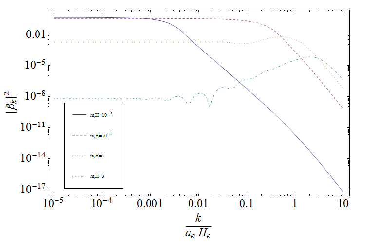
Figure 1: The Bogoliubov coefficient amplitude $|\beta_{k}|^{2}$ as a function of $k/(a_{e}H_{e})$ for various ratios of the fermion mass to the Hubble expansion rate during the dS era.

From these results, we first note that it can be determined that for heavy masses $m>H_{e}$, e.g. $m/H_{e}=1$ or 3, the infrared end of the spectrum behaves as $|\beta_{k}|^{2}\sim(1+\exp(2\pi m/H_{e}))^{-1}$. Further details of the heavy mass case are given in Appendix C. As the heavy mass situation is likely to be more sensitive to the abrupt transition approximation made in this section, we restrict our attention here to the light mass case in which $m<H_{e}$.

For the light mass case (e.g. $m/H_{e}=10^{-5}$ in Fig. (1)), we can see there are three ranges of $k$ that each have qualitatively different behavior. For $k/a_{e}>H_{e}$, the modes are still inside the horizon at the end of inflation, and the spectrum falls off as $|\beta_{k}|^{2}\propto k^{-6}$. In contrast, for $\sqrt{mH_{e}}<k/a_{e}<H_{e}$, the modes are outside of the horizon at the end of inflation and remain relativistic at the time when $m=H(\eta)$ during RD. In this case, the spectrum falls off as $|\beta_{k}|^{2}\propto k^{-4}$. Finally, for $k/a_{e}<\sqrt{mH_{e}}$, the modes are outside the horizon at the end of inflation and have become non-relativistic before $m=H(\eta)$ during RD. This results in a constant spectrum of $|\beta_{k}|^{2}\approx\frac{1}{2}$, in agreement with the results of Sec. III. Generically, if the scale factor $a(\eta)$ is sufficiently continuous Parker1971 ; Chung:2003wn , the spectrum will fall off in the ultraviolet region faster than $k^{-3}$, such that the total number density $n\sim\int d^{3}k|\beta_{k}|^{2}$ is finite. The majority of the contribution arises from the region in which $k/a_{e}<\sqrt{mH_{e}}$ where $|\beta_{k}|^{2}\approx\frac{1}{2}$, as anticipated in Sec. III. The number density for particle masses in the range of $m<0.1H_{e}$ is numerically determined to be (recall that $\eta_{m}$ is defined by $H(\eta_{m})=m$)

$$n(\eta)=4\times 0.005m^{3}\left(\frac{a(\eta_{m})}{a(\eta)}\right)^{3},$$ (43)

which again agrees with the analytic estimate of Eq. (33).

V Inflationary Reheating Dependence

We now consider the more realistic situation in which there is a smooth transition region between the dS and RD phases. When inflation ends, there is typically a period of coherent oscillations ($a_{e}<a<a_{\mbox{rh}}$) during which the equation of state is close to zero (see e.g. Kolb:1990vq ; Lyth:1998xn ; Mazumdar:2011zd ). During that period, the expansion rate behaves as $H\propto a^{-3/2}$ and not $a^{-2}$ as during RD. This difference will lead to an effective dilution of the dark matter particles by the time RD is reached. More precisely, the fermion number density will be diluted as $1/a^{3}$ as long as the fermion plus anti-fermion number is approximately conserved. As we will see below, the integrated dilution is typically a function of the reheating temperature during inflation.

Accounting for the dilution, in this section we estimate the relic abundance of fermionic particles (fermions plus anti-fermions). The dilution consideration breaks up naturally into two cases: $a_{\mbox{rh}}>a(t_{m})$ and $a_{\mbox{rh}}<a(t_{m})$. The former case corresponds to the situation in which the dominant particle production occurs during the reheating period, while the latter case corresponds to the complementary situation, which we will see below is unlikely to be physically important.

Let us begin with the case of $a_{\mbox{rh}}>a_{m}$, which corresponds to

$$H_{e}\gg m>H_{\mbox{rh}}\sim\frac{\sqrt{g_{*}}}{3}\frac{T_{\mbox{rh}}^{2}}{M_{p}}=\left(\frac{T_{\mbox{rh}}}{10^{9}\mbox{ GeV}}\right)^{2}\left(\frac{g_{*}}{100}\right)^{1/2}\mbox{GeV},$$ (44)

where $H_{\mbox{rh}}$ is the expansion rate at the time radiation domination is achieved. In this case, we have

$$\rho_{\Psi}(t_{\mbox{eq}})\sim 0.03m^{4}\left(\frac{H_{\mbox{rh}}}{m}\right)^{2}\left(\frac{a_{\mbox{rh}}}{a_{\mbox{eq}}}\right)^{3},$$ (45)

in which we have used the fact that $H\propto a^{-3/2}$ during reheating. We thus find the relic abundance today of fermionic particles to be

$$\Omega_{\psi}h^{2}\sim 3\left(\frac{m}{10^{11}\mbox{ GeV}}\right)^{2}\left(\frac{T_{\mbox{rh}}}{10^{9}\mbox{ GeV}}\right).$$ (46)

This matches Eq. (44) of Chung:2001cb (up to a factor of order of a few, part of which is expected from counting fermionic degrees of freedom), which was computed in the context of conformally coupled scalar fields. The match is interesting because the analog of Eq. (21) for the conformally coupled scalar field case has a different $k/a$ dependence that converts into an effective $m$ dependence due to the conformal invariance of the fermionic kinetic term. Eq. (46) also agrees with the model dependent numerical results of Kuzmin:1998kk up to a factor of 10. The related ratio of the fermion energy density to the radiation energy density at matter radiation equality, $\rho_{\Psi}(t_{\mbox{eq}})/\rho_{R}(t_{\mbox{eq}})$, is the same as Eq. (46) up to a factor of 10.

For the case with $a_{\mbox{rh}}<a_{m}$, we have

$$\rho_{\Psi}(t_{\mbox{eq}}) \sim 0.03m^{4}\left(\frac{a_{\mbox{m}}}{a_{\mbox{eq}}}\right)^{3},$$ (47)

which leads to

$$\frac{\rho_{\Psi}(t_{\mbox{eq}})}{\rho_{R}(t_{\mbox{eq}})}\sim\left(\frac{m}{10^{8}\mbox{ GeV}}\right)^{5/2}\left(\frac{g_{*}(t_{m})}{100}\right)^{-1/4}$$ (48)

which up to an order of magnitude is $\Omega_{\psi}$. However, since this applies only for

$$m<\left(\frac{T_{\mbox{rh}}}{10^{9}\mbox{ GeV}}\right)^{2}\left(\frac{g_{*}}{100}\right)^{1/2}\mbox{GeV},$$ (49)

the relic abundance is negligible in this case. For example, a $m\sim 1\,\mbox{GeV}$ benchmark point will render $\Omega_{\Psi}\sim 10^{-20}$.

VI Conclusions

In this paper, we revisited the gravitational production of massive Dirac fermions in inflationary cosmology. For the situation in which the fermions are light compared to the Hubble expansion rate at the end of inflation, we obtained the analytic result that the Bogoliubov coefficient amplitude $|\beta_{k}(t)|^{2}\sim 1/2$ if $H>m$ when $k/a\sim m$, as summarized in Eqs. (29) and (30). We used this result to compute the relic density assuming that the gravitationally produced fermions are superheavy dark matter particles. In cases of phenomenological interest, the dark matter relic abundance depends on the reheating temperature, as given in Eq. (46). Up to a multiplicative overall factor of $O(1)$, this result is identical to that obtained for conformally coupled scalars in Chung:2001cb . In the case that the fermions are heavy compared to the Hubble expansion rate at the end of inflation, the relic abundance is given by Eq. (94).

It is also of interest to consider the isocurvature behavior of the gravitationally produced fermions in the case that they have suitable long-range nongravitational interactions. Work along these lines is currently in progress ChungPengHojin .

Appendix A Formalism and Conventions

Here we follow the strategy outlined in the classical review paper of DeWitt DeWitt1975 . Consider the action of a four component Dirac spinor in curved spacetime:

$$S=\int d^{4}x\sqrt{|g(x)|}\bar{\Psi}(i\gamma^{a}\nabla_{e_{a}}-m)\Psi$$ (50)

in which the gamma matrices $\gamma^{a}$ are chosen to be in the Dirac basis

$$\gamma^{0}=\left(\begin{array}[]{cc}I&0\\ 0&-I\end{array}\right),\quad\gamma^{i}=\left(\begin{array}[]{cc}0&\sigma^{i}\\ -\sigma^{i}&0\end{array}\right)$$ (51)

to simplify the derivation of the second order differential equation of the spinor mode functions. Extremizing the action with respect to $\delta\bar{\Psi}$ and $\delta\Psi$ yields the equations of motion:

$$(i\gamma^{\alpha}\nabla_{e_{\alpha}}-m)\Psi=0,\qquad\nabla_{e_{a}}\bar{\Psi}(-i\gamma^{a})-\bar{\Psi}m=0.$$ (52)

The solution space can be endowed with a scalar product as

$$(\Psi_{1},\Psi_{2})_{\Sigma}=\int d\Sigma n_{\mu}e_{a}^{\,\mu}\bar{\Psi}_{1}\gamma^{a}\Psi_{2}$$ (53)

in which $\Sigma$ is an arbitrary space-like hypersurface, $d\Sigma$ is the volume 3-form on this hypersurface computed with the induced metric, and $n_{\mu}$ is the future-pointing time-like unit vector normal to $\Sigma$. The current conservation condition

$$\nabla_{e_{a}}(\bar{\Psi}_{1}\gamma^{a}\Psi_{2})=0$$ (54)

implies the integral in the scalar product is independent of the choice of $\Sigma$. The conjugation map can also be defined in the solution space as $Psi\mapsto-i\gamma^{2}\Psi^{*}$, which induces a pairing in the solution space.

Based on the scalar product and the conjugation map, one can construct an orthonormal basis for the solution space. It can be written as $\{U_{i},V_{i}\equiv-i\gamma^{2}U_{i}^{*}\}$ ($i$ labels different solutions), with

$$(U_{i},U_{j})=\delta_{ij},\qquad(U_{i},V_{j})=0.$$ (55)

The Heisenberg picture field operator $\Psi(x)$ can then be expanded in this basis as follows:

$$\Psi(x) = \sum_{i}a_{i}U_{i}+b_{i}^{\dagger}V_{i},$$ (56)

in which the canonical anticommutation relations imposed on equal-time surfaces and the orthonormality of the mode functions ensures that

$$\{a_{i},a_{j}^{\dagger}\}=\delta_{ij},\qquad\{b_{i},b_{j}^{\dagger}\}=\delta_{ij}.$$ (57)

The vacuum state is defined by $a_{i}|{\rm vac}\rangle=b_{i}|{\rm vac}\rangle=0$. The full Hilbert space can then be constructed as usual by applying the creation operators $a_{i}^{\dagger}$ and $b_{i}^{\dagger}$ to the vacuum state.

However, the choice of the orthonormal basis $\{U_{i},V_{i}\}$ is not unique. Consider a different orthonormal basis $\{\tilde{U}{}_{i},\tilde{V}{}_{i}\}$, which is related to the original basis as follows:

$$\tilde{U}{}_{i}=\sum_{j}\alpha_{ij}U_{j}+\beta_{ij}V_{j},\qquad\tilde{V}{}_{i}=\sum_{j}\alpha_{ij}^{*}V_{j}+\beta_{ij}^{*}U_{j}.$$ (58)

The Bogoliubov coefficients $\alpha_{ij}$ and $\beta_{ij}$ can be extracted as

$$\beta_{ij}=(V_{j},\tilde{U}{}_{i}),\qquad\alpha_{ij}=(U_{j},\tilde{U}{}_{i})$$ (59)

Note that the orthonormality relation on $\{U_{i},V_{i}\}$ and $\{\tilde{U}{}_{i},\tilde{V}{}_{i}\}$ implies the following relation:

$$\left(\begin{array}[]{cc}\alpha&\beta\\ \beta^{*}&\alpha^{*}\end{array}\right)^{*}\left(\begin{array}[]{cc}\alpha&\beta\\ \beta^{*}&\alpha^{*}\end{array}\right)^{T}=\left(\begin{array}[]{cc}I&0\\ 0&I\end{array}\right).$$ (60)

Using $\Psi=\sum_{i}a_{i}U_{i}+b_{i}^{\dagger}V_{i}=\sum_{i}\tilde{a_{i}}\tilde{U_{i}}+\tilde{b}_{i}^{\dagger}\tilde{V_{i}}$, the following relation is obtained:

$$\left(\begin{array}[]{c}\tilde{a}\\ \tilde{b}^{\dagger}\end{array}\right)=\left(\begin{array}[]{cc}\alpha^{*}&\beta^{*}\\ \beta&\alpha\end{array}\right)\left(\begin{array}[]{c}a\\ b^{\dagger}\end{array}\right).$$ (61)

Hence, the two mode functions result in inequivalent vacua. To see this more explicitly, consider the expectation value of the occupation number operator $\tilde{a_{i}}^{\dagger}\tilde{a_{i}}$ with respect to the vacuum defined using the $a_{i},b_{i}$ operators:

$$\langle{\rm vac}|\tilde{a_{i}}^{\dagger}\tilde{a_{i}}|{\rm vac}\rangle = \sum_{j}|\beta_{ij}|^{2}.$$ (62)

The vacuum state corresponding to one definition thus is an excited state in the other definition.

We turn now to FRW spacetime, in which the metric is conformally flat:

$$ds^{2}=g_{\mu\nu}dx^{\mu}dx^{\nu}=a(x_{0})^{2}\eta_{\mu\nu}dx^{\mu}dx^{\nu}.$$ (63)

Since the action of Eq. (50) is covariant under Weyl transformations:

$$g_{\mu\nu}=\Omega^{2}(x)\tilde{g}_{\mu\nu},\,\,\Psi=\Omega(x)^{-3/2}\tilde{\psi},\qquad e_{a}^{\,\,\mu}=\Omega(x)^{-1}\tilde{e}_{a}^{\,\,\mu},$$ (64)

a Weyl transformation with $\Omega(x)=a(x_{0})$ can be used to rewrite the action as follows:

$$S=\int d^{4}x\bar{\psi}(i\gamma^{\mu}\partial_{\mu}-a(\eta)m)\psi,$$ (65)

where $\eta$ is the conformal time and $\psi$ is the rescaled spinor field. The equation of motion now takes the form

$$(i\gamma^{\mu}\partial_{\mu}-a(\eta)m)\psi=0.$$ (66)

The solution space is spanned by the orthonormal basis $\{U_{\vec{k},r},V_{\vec{k},r}\}$, which can be written as follows:

$$U_{\vec{k},r}(\eta,\vec{x}) = \frac{e^{i\vec{k}\cdot\vec{x}}}{(2\pi)^{3/2}}\left(\begin{array}[]{c}u_{A,k,\eta}h_{\hat{k},r}\\ r\,u_{B,k,\eta}h_{\hat{k},r}\end{array}\right)$$ (69)

$$\equiv \frac{e^{i\vec{k}\cdot\vec{x}}}{(2\pi)^{3/2}}\left(\begin{array}[]{c}u_{A,k,\eta}\\ r\,u_{B,k,\eta}\end{array}\right)\otimes h_{\hat{k},r},$$ (72)

in which $\hat{k}$ is the unit vector in the $\vec{k}$ direction ($\hat{k}=\hat{e}_{z}$ if $\vec{k}=0$), and $h_{\hat{k},r}$ is a 2-component complex column vector (called the helicity 2-spinor) that satisfies

$$\hat{k}\cdot\vec{\sigma}h_{\hat{k},r}=rh_{\hat{k},r},\,r=\pm 1.$$ (73)

More concretely, if $\hat{k}=(\theta,\phi)$ in spherical coordinates, then the normalization factor can be chosen such that

$$h_{\hat{k},+1}\equiv\left(\begin{array}[]{c}\cos\frac{\theta}{2}e^{-i\phi}\\ \sin\frac{\theta}{2}\end{array}\right),h_{\hat{k},-1}\equiv\left(\begin{array}[]{c}\sin\frac{\theta}{2}e^{-i\phi}\\ -\cos\frac{\theta}{2}\end{array}\right).$$ (74)

One can easily check that due to this phase convention

$$-i\sigma^{2}(h_{\hat{k},r})^{*}=-re^{-ir\phi}h_{\hat{k},-r},\qquad h_{-\hat{k},r}=-h_{\hat{k},-r}.$$ (75)

Using the above relations, one obtains

$$V_{\vec{k},r}(\eta,\vec{x})=\frac{e^{-i\vec{k}\cdot\vec{x}}}{(2\pi)^{3/2}}\left(\begin{array}[]{c}-u_{B,k,\eta}^{*}\\ ru_{A,k,\eta}^{*}\end{array}\right)\otimes h_{-\hat{k},r}\cdot(e^{-ir\phi}).$$ (76)

The normalization of the mode functions implies

$$h_{\hat{k},r}^{\dagger}h_{\hat{k},s}=\delta_{rs},\qquad|u_{A,k,\eta}|^{2}+|u_{B,k,\eta}|^{2}=1.$$ (77)

With this ansatz, Eq. (66) simplifies as follows:

$$i\partial_{\eta}\left(\begin{array}[]{c}u_{A}\\ u_{B}\end{array}\right)=\left(\begin{array}[]{cc}am&k\\ k&-am\end{array}\right)\left(\begin{array}[]{c}u_{A}\\ u_{B}\end{array}\right).$$ (78)

Let $\tilde{U}_{\vec{k},s}$ be another basis in the form of Eq. (72). Due to the orthogonality of $h_{\hat{k},r}$ and $e^{i\vec{k}\cdot x}$ , $\tilde{U}_{\vec{k},s}$ can only be a linear combination of $U_{\vec{k},s},V_{-\vec{k},s}$:

$$\tilde{U}_{\vec{k},s}=\alpha_{(\vec{k},s)(\vec{k},s)}U_{\vec{k},s}+\beta_{(\vec{k},s)(-\vec{k},s)}V_{-\vec{k},s}$$ (79)

The Bogoliubov coefficients are extracted using the scalar product of the mode functions evaluated at time $\eta$ as follows:

$$\alpha_{(\vec{k},s)(\vec{k},s)} = u_{A,k,\eta}^{*}\tilde{u}_{A,k,\eta}+u_{B,k,\eta}^{*}\tilde{u}_{B,k,\eta}$$ (80)

$$\beta_{(\vec{k},s)(-\vec{k},s)} = e^{-is\phi(\hat{k})}(u_{A,k,\eta}\tilde{u}_{B,k,\eta}-u_{B,k,\eta}\tilde{u}_{A,k,\eta})$$ (81)

Since we will only consider $|\beta_{k}|^{2}$ in this work, we can drop the $e^{-is\phi(\hat{k})}$ factor in the $\beta_{k}$ definition without loss of generality. Here one of the bases (corresponding to the Heisenberg state of the universe) is specified by asymptotic conditions such as the Bunch-Davies boundary condition as the in-vacuum (see e.g. Eq. (35).) Similarly, the other basis is the observable operator basis as specified by asymptotic conditions at late times, which is referred to as the out-vacuum.

Appendix B Demonstration that $|\beta_{k}|^{2}\sim\frac{1}{2}$ for Small $k$

We begin with the determination of $\beta_{k}$ from Eq. (81) evaluated at very late times when the out-modes can be directly replaced by their asymptotic values. In the limit in which $am/k\rightarrow\infty$, we see that we then only need to find the asymptotic values of the in-modes:

$$|\beta_{k}|=|u_{A,k,\eta}^{out}u_{B,k,\eta}^{in}-u_{B,k,\eta}^{out}u_{A,k,\eta}^{in}|=|\sqrt{\frac{\omega+am}{2\omega}}u_{B,k,\eta}^{in}-\sqrt{\frac{\omega-am}{2\omega}}u_{A,k,\eta}^{in}|=\lim_{\eta\rightarrow\infty}|u_{B,k,\eta}^{in}|.$$ (82)

Let us consider the evolution equations as given in Eq. (78) with boundary conditions as given in Eq. (35). For concreteness, we choose a time $\eta_{i}$ that is early enough such that $u_{A}(\eta_{i})\approx u_{B}(\eta_{i})\approx\frac{1}{\sqrt{2}}$. The system can be formally solved to obtain

$$\left(\begin{array}[]{c}u_{A}\\ u_{B}\end{array}\right)_{f} = T\exp\left\{-i\int d\Phi\sigma(\theta)\right\}\left(\begin{array}[]{c}u_{A}\\ u_{B}\end{array}\right)_{i}$$ (87)

in which $\omega\cos\theta=k$, $\omega\sin\theta=am$, $\omega d\eta=d\Phi$, and $\sigma(\theta)=\sigma_{1}\cos\theta+\sigma_{3}\sin\theta$ ($0\leq\theta\leq\pi/2$). The time evolution is thus expressed as a series of infinitesimal $SU(2)$ rotations that act successively on the complex vector $u\equiv(u_{A}\,u_{B})$.

For fixed $\theta$, the evolution corresponds to precession about the axis defined by $\sigma(\theta)$. However, throughout the evolution of the universe, $\sigma(\theta)$ evolves from its initial direction along $\sigma_{1}$ ($am\ll k$) to its final direction along $\sigma_{3}$ ($am\gg k$). If the switching of the axis is much faster than the precession time scale, $u$ remains in the $xy$-plane and rotates around the new axis $\sigma_{3}$, while if the switching is much slower compared with the precession time scale, $u$ adheres closely to the rotation axis and thus ends up in the $\sigma_{3}$ direction. The time scale of the axis switching is given by the Hubble expansion rate, since the universe needs to expand several e-folds for $am$ to overtake $k$, while the time scale of the precession is given by the physical frequency $\omega/a$, which is on the order of $m$ during the transition. Hence, fast transitions occur when $m\ll H$, for which $|u_{B}|^{2}$ stabilizes at $\frac{1}{2}$ and $|\beta_{k}|^{2}=\frac{1}{2}$. After $H(\eta)$ drops below $m$, only slow transitions occur and $|\beta_{k}|^{2}$ is small.

Appendix C Heavy mass case ($m>H_{e})$

As we expect the particle production spectrum $|\beta_{k}|^{2}$ to be exponentially suppressed by $m/H$, we can adopt a similar approach as the heavy mass scalar case Chung2003 to look for a one-pole approximation to the time integral that determines $\beta_{k}$. We shall consider the time-dependent Bogoliubov coefficients between the in-modes and the zeroth adiabatic modes with boundary conditions such that

$$\left(\begin{array}[]{c}u_{A}\\ u_{B}\end{array}\right)_{k,\eta=\eta_{1}}^{(\eta_{1})}=\left(\begin{array}[]{c}\sqrt{\frac{\omega+am}{2\omega}}\\ \sqrt{\frac{\omega-am}{2\omega}}\end{array}\right).$$ (88)

In the above, the superscript $(\eta_{1})$ indicates the time that the boundary conditions are imposed. The in-modes can be decomposed into the zeroth adiabatic mode basis as follows:

$$\left(\begin{array}[]{c}u_{A}\\ u_{B}\end{array}\right)_{k,\eta_{1}}^{in}=\alpha_{k}^{in-(\eta_{1})}\left(\begin{array}[]{c}u_{A}\\ u_{B}\end{array}\right)_{k,\eta_{1}}^{(\eta_{1})}+\beta_{k}^{in-(\eta_{1})}\left(\begin{array}[]{c}-u_{B}^{*}\\ u_{A}^{*}\end{array}\right)_{k,\eta_{1}}^{(\eta_{1})}.$$ (89)

For $\eta_{1}\rightarrow\infty$, the instantaneous-modes will coincide with the out-modes up to an overall phase, and hence

$$|\beta_{k}|=\lim_{\eta_{1}\rightarrow\infty}|\beta_{k}^{in-(\eta_{1})}|.$$ (90)

Inserting this decomposition into Eq. (78) (and writing $\alpha_{k}^{in-(\eta_{1})}$ as $\alpha_{k}(\eta_{1})$, etc. for notational simplicity) results in

$$\dot{\alpha}_{k}(\eta_{1})=-\frac{mk}{2\omega^{2}}\dot{a}e^{2i\int^{\eta_{1}}d\eta\omega(\eta)}\beta_{k}(\eta_{1}),\qquad\dot{\beta}_{k}(\eta_{1})=\frac{mk}{2\omega^{2}}\dot{a}e^{-2i\int^{\eta_{1}}d\eta\omega(\eta)}\alpha_{k}(\eta_{1}),$$ (91)

with the initial conditions $\alpha_{k}(\eta_{i})=1,\,\beta_{k}(\eta_{i})=0$ for the time $\eta_{i}$ early enough that the mode is inside the dS event horizon. Since we expect $|\beta_{k}|\ll 1$ and $a_{k}\approx 1$, we can replace $\alpha=1$ in Eq. (91) and formally write the solution as

$$\beta_{k}(\eta_{f})=\int_{\eta_{i}}^{\eta_{f}}d\tau\frac{mk}{2\omega^{2}}\dot{a}(\tau)e^{-2i\int^{\tau}d\eta\omega(\eta)}.$$ (92)

The steepest descent method can be applied to evaluate this integral in a similar fashion as was done for the scalar case in Chung2003 . Despite the different $k$ dependence in Eq. (92), the result is the same as Eq. (41) of Chung2003 :

$$|\beta_{k}|^{2}\approx\exp\left\{-4\left[\frac{[k/a(r)]^{2}}{m\sqrt{H^{2}(r)+R(r)/6}}+\frac{m}{\sqrt{H^{2}(r)+R(r)/6}}\right]\right\},$$ (93)

in which $r$ is the real part of the complexified conformal time $\tilde{\eta}$ at which $\omega(\tilde{\eta})=0$ and $R$ is the Ricci scalar. This is approximately due to the fact that the branch point occurs when $\omega=0$, such that the dominant contribution occurs when $|k/a|\sim m$. Eq. (93) leads to the particle number density (fermion plus anti-fermion) as

$$\rho_{\psi}(t)\approx\frac{1}{2\pi^{3/2}}\left(\frac{a(r)}{a(t)}\right)^{3}m\left[\frac{m}{4}\sqrt{H^{2}(r)+R(r)/6}\right]^{3/2}\exp\left(\frac{-4m}{\sqrt{H^{2}(r)+R(r)/6}}\right).$$ (94)

To estimate the relic abundance from this equation, one can use the formula

$$\Omega_{\psi}h^{2}\sim 100\left(\frac{T_{\mbox{rh}}}{10^{9}\mbox{GeV}}\right)\left(\frac{H(t_{e})}{10^{13}\mbox{GeV}}\right)^{-2}\frac{\rho_{\psi}(t_{e})}{\left(10^{12}\mbox{GeV}\right)^{4}},$$ (95)

where one is only formally evaluating the $\rho_{\psi}(t_{e})$ at the end of inflation time $t_{e}$ even though the particle densities are well defined at times far later than time. Unlike the formulae presented in the body of the text, the exponential sensitivity and the approximations made in obtaining the saddle-point does not allow one to guarantee an order of magnitude numerical accuracy, especially for large $m/H(r)$ Chung2003 . However, the spectral and mass cutoffs can be well estimated by Eqs. (93) and (94).

- (1) N. Birrell and P. Davies, QUANTUM FIELDS IN CURVED SPACE, .
- (2) B. S. DeWitt, Quantum Field Theory in Curved Space-Time, Phys.Rept. 19 (1975) 295–357.
- (3) A. E. Lawrence and E. J. Martinec, String field theory in curved space-time and the resolution of space - like singularities, Class.Quant.Grav. 13 (1996) 63–96, [hep-th/9509149].
- (4) S. S. Gubser, String production at the level of effective field theory, Phys.Rev. D69 (2004) 123507, [hep-th/0305099].
- (5) N. Turok, M. Perry, and P. J. Steinhardt, M theory model of a big crunch / big bang transition, Phys.Rev. D70 (2004) 106004, [hep-th/0408083].
- (6) J. J. Friess, S. S. Gubser, and I. Mitra, String creation in cosmologies with a varying dilaton, Nucl.Phys. B689 (2004) 243–256, [hep-th/0402156].
- (7) A. J. Tolley and D. H. Wesley, String pair production in a time-dependent gravitational field, Phys.Rev. D72 (2005) 124009, [hep-th/0509151].
- (8) S. Cremonini and S. Watson, Dilaton dynamics from production of tensionless membranes, Phys.Rev. D73 (2006) 086007, [hep-th/0601082].
- (9) S. R. Das and J. Michelson, Matrix membrane big bangs and D-brane production, Phys.Rev. D73 (2006) 126006, [hep-th/0602099].
- (10) C.-J. Feng, X. Gao, M. Li, W. Song, and Y. Song, Reheating and cosmic string production, Nucl.Phys. B800 (2008) 190–203, [arXiv:0707.0908].
- (11) J. S. Schwinger, On gauge invariance and vacuum polarization, Phys.Rev. 82 (1951) 664–679.
- (12) E. Brezin and C. Itzykson, Pair production in vacuum by an alternating field, Phys.Rev. D2 (1970) 1191–1199.
- (13) J. Audretsch and G. Schaefer, Thermal Particle Production in a Radiation Dominated Robertson-Walker Universe, J.Phys.A A11 (1978) 1583–1602.
- (14) S. G. Mamaev and V. M. Mostepanenko, Particle creation by the gravitational field, and the problem of the cosmological singularity, Pis ma Astronomicheskii Zhurnal 4 (June, 1978) 203–206.
- (15) S. G. Mamaev, V. M. Mostepanenko, and V. M. Frolov, Fermion pair creation near the Friedmann singularity, Soviet Astronomy Letters 1 (Oct., 1975) 179–+.
- (16) L. Parker, Quantized fields and particle creation in expanding universes. 2., Phys.Rev. D3 (1971) 346–356.
- (17) L. Parker, Quantized fields and particle creation in expanding universes. 1., Phys.Rev. 183 (1969) 1057–1068.
- (18) V. A. Kuzmin and I. I. Tkachev, Ultrahigh-energy cosmic rays and inflation relics, Phys.Rept. 320 (1999) 199–221, [hep-ph/9903542].
- (19) S. V. Anischenko, S. L. Cherkas, and V. L. Kalashnikov, Cosmological production of fermions in a flat Friedman universe with linearly growing scale factor: Exactly solvable model, Nonlin.Phenom.Complex Syst. 13 (2010) 315–319, [arXiv:0911.0769].
- (20) S. Tsujikawa and H. Yajima, Massive fermion production in nonsingular superstring cosmology, Phys. Rev. D 64 (Jun, 2001) 023519.
- (21) D. J. Chung, E. W. Kolb, and A. Riotto, Superheavy dark matter, Phys.Rev. D59 (1999) 023501, [hep-ph/9802238]. In *Venice 1999, Neutrino telescopes, vol. 2* 217-237.
- (22) V. Kuzmin and I. Tkachev, Matter creation via vacuum fluctuations in the early universe and observed ultrahigh-energy cosmic ray events, Phys.Rev. D59 (1999) 123006, [hep-ph/9809547].
- (23) J. R. Ellis, J. L. Lopez, and D. V. Nanopoulos, Confinement of fractional charges yields integer charged relics in string models, Phys.Lett. B247 (1990) 257.
- (24) K. Benakli, J. R. Ellis, and D. V. Nanopoulos, Natural candidates for superheavy dark matter in string and M theory, Phys.Rev. D59 (1999) 047301, [hep-ph/9803333].
- (25) A. Kusenko and M. E. Shaposhnikov, Supersymmetric Q balls as dark matter, Phys.Lett. B418 (1998) 46–54, [hep-ph/9709492].
- (26) T. Han, T. Yanagida, and R.-J. Zhang, Adjoint messengers and perturbative unification at the string scale, Phys.Rev. D58 (1998) 095011, [hep-ph/9804228].
- (27) G. Dvali, Infrared hierarchy, thermal brane inflation and superstrings as superheavy dark matter, Phys.Lett. B459 (1999) 489–496, [hep-ph/9905204].
- (28) K. Hamaguchi, K. Izawa, Y. Nomura, and T. Yanagida, Longlived superheavy particles in dynamical supersymmetry breaking models in supergravity, Phys.Rev. D60 (1999) 125009, [hep-ph/9903207].
- (29) C. Coriano, A. E. Faraggi, and M. Plumacher, Stable superstring relics and ultrahigh-energy cosmic rays, Nucl.Phys. B614 (2001) 233–253, [hep-ph/0107053].
- (30) H.-C. Cheng, K. T. Matchev, and M. Schmaltz, Radiative corrections to Kaluza-Klein masses, Phys.Rev. D66 (2002) 036005, [hep-ph/0204342].
- (31) G. Shiu and L.-T. Wang, D matter, Phys.Rev. D69 (2004) 126007, [hep-ph/0311228].
- (32) V. Berezinsky, M. Kachelriess, and M. Solberg, Supersymmetric superheavy dark matter, Phys.Rev. D78 (2008) 123535, [arXiv:0810.3012].
- (33) T. W. Kephart and Q. Shafi, Family unification, exotic states and magnetic monopoles, Phys.Lett. B520 (2001) 313–316, [hep-ph/0105237].
- (34) T. W. Kephart, C.-A. Lee, and Q. Shafi, Family unification, exotic states and light magnetic monopoles, JHEP 0701 (2007) 088, [hep-ph/0602055].
- (35) C. Barbot and M. Drees, Detailed analysis of the decay spectrum of a super-heavy X particle, Astropart. Phys. 20 (2003) 5–44, [hep-ph/0211406].
- (36) I. F. Albuquerque and L. Baudis, Direct detection constraints on superheavy dark matter, Phys.Rev.Lett. 90 (2003) 221301, [astro-ph/0301188].
- (37) M. Taoso, G. Bertone, and A. Masiero, Dark Matter Candidates: A Ten-Point Test, JCAP 0803 (2008) 022, [arXiv:0711.4996]. * Brief entry *.
- (38) J. Bovy and G. R. Farrar, Connection between a possible fifth force and the direct detection of Dark Matter, Phys.Rev.Lett. 102 (2009) 101301, [arXiv:0807.3060].
- (39) I. F. Albuquerque and C. Perez de los Heros, Closing the Window on Strongly Interacting Dark Matter with IceCube, Phys.Rev. D81 (2010) 063510, [arXiv:1001.1381].
- (40) D. J. Chung, Classical inflation field induced creation of superheavy dark matter, Phys.Rev. D67 (2003) 083514, [hep-ph/9809489].
- (41) D. J. Chung, P. Crotty, E. W. Kolb, and A. Riotto, On the gravitational production of superheavy dark matter, Phys.Rev. D64 (2001) 043503, [hep-ph/0104100].
- (42) B. Garbrecht, T. Prokopec, and M. G. Schmidt, Particle number in kinetic theory, Eur.Phys.J. C38 (2004) 135–143, [hep-th/0211219].
- (43) S. A. Ramsey, B. L. Hu, and A. M. Stylianopoulos, Nonequilibrium inflaton dynamics and reheating. ii. fermion production, noise, and stochasticity, Phys. Rev. D 57 (May, 1998) 6003–6021.
- (44) B. A. Bassett, M. Peloso, L. Sorbo, and S. Tsujikawa, Fermion production from preheating amplified metric perturbations, Nucl.Phys. B622 (2002) 393–415, [hep-ph/0109176].
- (45) M. Peloso and L. Sorbo, Preheating of massive fermions after inflation: Analytical results, JHEP 0005 (2000) 016, [hep-ph/0003045].
- (46) J. Garcia-Bellido, S. Mollerach, and E. Roulet, Fermion production during preheating after hybrid inflation, JHEP 0002 (2000) 034, [hep-ph/0002076].
- (47) J. Baacke, K. Heitmann, and C. Pätzold, Nonequilibrium dynamics of fermions in a spatially homogeneous scalar background field, Phys. Rev. D 58 (Nov, 1998) 125013.
- (48) P. B. Greene and L. Kofman, Preheating of fermions, Phys.Lett. B448 (1999) 6–12, [hep-ph/9807339].
- (49) A. D. Dolgov and D. P. Kirilova, Production of particles by a variable scalar field, Sov. J. Nucl. Phys. 51 (1990) 172–177. [Yad.Fiz.51:273-282,1990].
- (50) D. J. Chung, E. W. Kolb, A. Riotto, and I. I. Tkachev, Probing Planckian physics: Resonant production of particles during inflation and features in the primordial power spectrum, Phys.Rev. D62 (2000) 043508, [hep-ph/9910437].
- (51) B. Garbrecht and T. Prokopec, Fermion mass generation in de sitter space, Phys. Rev. D 73 (Mar, 2006) 064036.
- (52) A. L. Maroto and A. Mazumdar, Production of spin 3/2 particles from vacuum fluctuations, Phys. Rev. Lett. 84 (2000) 1655–1658, [hep-ph/9904206].
- (53) R. Kallosh, L. Kofman, A. D. Linde, and A. Van Proeyen, Gravitino production after inflation, Phys.Rev. D61 (2000) 103503, [hep-th/9907124].
- (54) G. Giudice, A. Riotto, and I. Tkachev, Thermal and nonthermal production of gravitinos in the early universe, JHEP 9911 (1999) 036, [hep-ph/9911302].
- (55) H. P. Nilles, M. Peloso, and L. Sorbo, Coupled fields in external background with application to nonthermal production of gravitinos, JHEP 04 (2001) 004, [hep-th/0103202].
- (56) H. P. Nilles, M. Peloso, and L. Sorbo, Nonthermal production of gravitinos and inflatinos, Phys. Rev. Lett. 87 (2001) 051302, [hep-ph/0102264].
- (57) M. Kawasaki, F. Takahashi, and T. T. Yanagida, The gravitino overproduction problem in inflationary universe, Phys. Rev. D74 (2006) 043519, [hep-ph/0605297].
- (58) D. J. Chung, A. Notari, and A. Riotto, Minimal theoretical uncertainties in inflationary predictions, JCAP 0310 (2003) 012, [hep-ph/0305074].
- (59) E. W. Kolb and M. S. Turner, The Early universe, Front.Phys. 69 (1990) 1–547.
- (60) D. H. Lyth and A. Riotto, Particle physics models of inflation and the cosmological density perturbation, Phys.Rept. 314 (1999) 1–146, [hep-ph/9807278].
- (61) A. Mazumdar, The origin of dark matter, matter-anti-matter asymmetry, and inflation, arXiv:1106.5408. * Temporary entry *.
- (62) D. J. H. Chung, H. Yoo, and P. Zhou in preparation.