METHOD OF ANALYTIC EVOLUTION OF FLAT DISTRIBUTION AMPLITUDES IN QCD

Abstract

A new analytical method of performing ERBL evolution is described. The main goal is to develop an approach that works for distribution amplitudes that do not vanish at the end points, for which the standard method of expansion in Gegenbauer polynomials is inefficient. Two cases of the initial DA are considered: a purely flat DA, given by the same constant for all $x$, and an antisymmetric DA given by opposite constants for $x\gtrless 1/2$. For a purely flat DA, the evolution is governed by an overall $(x\bar{x})^{t}$ dependence on the evolution parameter $t$ times a factor that was calculated as an expansion in $t$. For an antisymmetric flat DA, an extra overall factor $|1-2x|^{2t}$ appears due to a jump at $x=1/2$. A good convergence was observed in the $t\lesssim 1/2$ region. For larger $t$, one can use the standard method of the Gegenbauer expansion.

PACS numbers: 12.38.-t, 11.10.-z

1 Introduction

Recent BaBar data[1] on the $\gamma^{*}\gamma\to\pi^{0}$ transition form factor correspond to approximately logarithmic $\ln Q^{2}$ raise of the combination $Q^{2}F_{\gamma^{*}\gamma\pi^{0}}(Q^{2})$ in the region of very high momentum transfers 10 to 40 GeV², where perturbative QCD approach[2] predicts nearly constant behavior for this combination. It was proposed[3, 4] to explain the BaBar “puzzle” by assuming that the pion distribution amplitude (DA) is “flat”: $\varphi_{\pi}(x)=f_{\pi}$.

In general, DAs $\varphi_{\pi}(x,\mu)$ depend on the normalization scale $\mu$, tending to the “asymptotic” shape $\varphi_{\pi}^{\rm as}(x)=6f_{\pi}x(1-x)$ in the $\mu\to\infty$ limit, for any intial pion DA. A standard way[5, 2] to this result is to expand the initial pion DA over the eigenfunctions $x(1-x)C_{n}^{3/2}(2x-1)$ of the evolution kernel. Each Gegenbauer projection then changes as $[\ln\ln(\mu_{0}/\Lambda)/\ln\ln(\mu/\Lambda)]^{\gamma_{n}/\beta_{0}}$ when $\mu$ increases. All anomalous dimensions $\gamma_{n}$ are positive, except for $\gamma_{0}$ which is zero, hence only the $\sim x(1-x)$ part survives. For a pion DA given by a sum of a few Gegenbauer polynomials, this method gives a convenient analytic expression for the DA evolution. However, to get a flat pion DA, one should formally take an infinite number of Gegenbauer polynomials (this difficulty was mentioned in a recent paper[6]), and one should take a very large number of terms to get a reasonably precise (point by point) result for the evolved DA. In fact, a long time ago, it was established[5] that, if the initial pion DA $\varphi_{\pi}(x,\mu_{0})$ has a $\sim[x(1-x)]^{r}$ form near the end points $x=0,1$, with a small $r$, then evolution just increases this power:

$$r\to r(\mu)=r(\mu_{0})+2C_{F}\ln[\ln(\mu/\Lambda)/\ln(\mu_{0}/\Lambda)]/\beta_{0}\ .$$

This result was obtained by incorporating the large-$n$ behavior $\gamma_{n}\sim 4C_{F}\ln n$ of the anomalous dimensions in QCD, and summation of the leading end-point region terms. Thus, one may expect that the evolved form of the flat pion DA should be close to $[x(1-x)]^{2C_{F}\ln[\ln(\mu/\Lambda)/\ln(\mu_{0}/\Lambda)]/\beta_{0}}$. In particular, this statement was repeated in a more recent paper[7] on the basis of an analysis similar to that of Ref.[Efremov:1979qk].

Our goal is to develop a method that allows one to get explicit analytic expressions for the evolution of the flat distribution amplitude in QCD. As we will see, our results not only confirm the above expectation, but also provide a regular way of calculating corrections to it. We also apply this new method to obtain the evolution of the DA $d(x)\sim{\rm sgn}(x-1/2)$ that is antisymmetric with respect to the central point $x=1/2$. Such DA may correspond to the so-called “D-term”[8] in generalized parton distributions.

2 Evolution of Flat DA

2.1 Evolution equation

Evolution of the pion DA in the leading logarithm approximation is governed by

$$\frac{\partial\varphi(x,t)}{\partial t}=\int_{0}^{1}[V(x,y)]_{+}\,\varphi(y,t)dy,$$ (1)

where $t=2C_{F}\ln\ln(\mu/\Lambda)/b_{0}$ is the leading logarithm QCD evolution parameter, and $[V(x,y)]_{+}$ is the evolution kernel which has the property of a plus distribution

$$[V(x,y)]_{+}=V(x,y)-\delta(y-x)\int_{0}^{1}V(z,y)dz$$ (2)

with respect to its first argument. In our case,

$$V(x,y)=\left[\frac{x}{y}\left(1+\frac{1}{y-x}\right)\right]\theta(x<y)+\left[\frac{\bar{x}}{\bar{y}}\left(1+\frac{1}{x-y}\right)\right]\theta(y<x)\ ,$$ (3)

where we use a standard notation $\bar{x}=1-x$ and $\bar{y}=1-y$. One may rewrite the evolution equation as

$$\frac{\partial\varphi(x,t)}{\partial t}=\int_{0}^{1}\left[V(x,y)\varphi(y,t)-V(y,x)\,\varphi(x,t)\right]\,dy\ .$$ (4)

It is clear that the singularities of $V(x,y)$ and $V(y,x)$ at $x=y$ cancel each other in the integrand above, even though the subtraction there does not look like a “+”-prescription with respect to the integration variable. Adding and subtracting $V(x,y)\varphi(x)$ in the integrand, we obtain the equation

$$\frac{\partial\varphi(x,t)}{\partial t}=\int_{0}^{1}V(x,y)[\varphi(y,t)-\varphi(x,t)]dy-\varphi(x,t)\int_{0}^{1}[V(y,x)-V(x,y)]dy$$ (5)

in which the first term has the structure of the “+”-prescription with respect to the integration variable, so that $1/(x-y)$ singularity of $V(x,y)$ is cancelled by zero of $\varphi(y,t)-\varphi(x,t)$ at $x=y$. The integral in the second term (call it $-v(x)$) is also finite. Taking the Ansatz

$$\varphi(x,t)=e^{tv(x)}\Phi(x,t)\ ,$$ (6)

we obtain for $\Phi(x,t)$ the equation

$$\frac{\partial{\Phi(x,t)}}{\partial t}=\int_{0}^{1}V(x,y)[e^{t[v(y)-v(x)]}\Phi(y,t)-\Phi(x,t)]\,dy\,,$$ (7)

which does not have the second term. The solution for $\Phi(x,t)$ may be written as a series in $t$

$$\Phi(x,t)=\sum_{n=0}^{\infty}\frac{t^{n}}{n!}\Phi_{n}(x)\,,$$ (8)

with the functions $\Phi_{n}(x)$ satisfying the recurrence relation

$$\Phi_{n+1}(x)=\int_{0}^{1}V(x,y)\left[\sum_{l=0}^{n}\frac{n!}{(n-l)!\,l!}\Phi_{l}(y)\left[v(y)-v(x)\right]^{n-l}-\Phi_{n}(x)\right]dy\ .$$ (9)

2.2 Singular Part

It is instructive to consider first an auxiliary situation when the evolution kernel is given by the singular part only

$$V^{\text{sing}}(x,y) = \left(\frac{x}{y(y-x)}\right)\theta(x<y)+(x\rightarrow\bar{x},\,\,\,y\rightarrow\bar{y})$$ (10)

of the QCD kernel. In this case

$$v^{\text{sing}}(x)\equiv-\int_{0}^{1}[V^{\text{sing}}(y,x)-V^{\text{sing}}(x,y)]dy=2+\ln(x\bar{x})$$ (11)

and the recurrence relation is given by

$$\Phi_{n+1}(x)=\int_{0}^{1}V(x,y)\left[\sum_{l=0}^{n}\frac{n!}{(n-l)!\,l!}\Phi_{l}(y)\left(\ln\frac{y\bar{y}}{x\bar{x}}\right)^{n-l}-\Phi_{n}(x)\right]dy\ ,$$ (12)

or, explicitly for the first terms,

$$\Phi_{1}(x) = \int_{0}^{1}V(x,y)[\Phi_{0}(y)-\Phi_{0}(x)]dy\,,$$ (13)

$$\Phi_{2}(x) = \int_{0}^{1}V(x,y)\left[\Phi_{0}(y)\ln\left(\frac{y\bar{y}}{x\bar{x}}\right)+\Phi_{1}(y)-\Phi_{1}(x)\right]dy\,,$$ (14)

$$\Phi_{3}(x) = \int_{0}^{1}V(x,y)\left[\Phi_{0}(y)\ln^{2}\left(\frac{y\bar{y}}{x\bar{x}}\right)+2\Phi_{1}(y)\ln\left(\frac{y\bar{y}}{x\bar{x}}\right)+\Phi_{2}(y)-\Phi_{2}(x)\right]dy\,.\ \ \$$ (15)

In this approximation, we can write

$$\varphi^{\text{sing}}(x,t) = (x\bar{x})^{t}\,e^{2t}\,\left(\Phi_{0}(x)+t\Phi_{1}(x)+\frac{t^{2}}{2!}\Phi_{2}(x)+\frac{t^{3}}{3!}\Phi_{3}(x)+\ldots\right)\ .$$ (16)

If we take the flat DA for $t=0$, i.e., $\Phi(x,0)=1$, this gives

$$\Phi_{0}(x) = 1\,$$ (17)

$$\Phi_{1}(x) = 0\,$$ (18)

$$\Phi_{2}(x) = -2\ln x\ln\bar{x}$$ (19)

$$\Phi_{3}(x) = 3\ln(x\bar{x})\ln x\ln\bar{x}+2\left[\ln x\,\text{Li}_{2}(x)+\ln\bar{x}\,\text{Li}_{2}(\bar{x})\right]$$ (20)

$$-4\,\left[\text{Li}_{3}(x)+\,\text{Li}_{3}(\bar{x})\right]+8\zeta(3)$$

The graphical results for the expansion components are given in Fig.1.

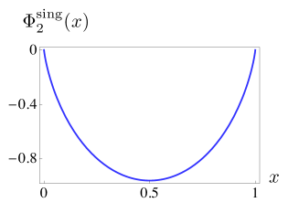
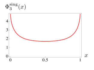
Figure 1: Expansion components $\Phi^{\text{sing}}_{2}(x)$ (a) and $\Phi^{\text{sing}}_{3}(x)$ (b).

As far as $\int_{0}^{1}[V(x,y)]_{+}dx=0$, evolution does not change the normalization integral for $\varphi(x,t)$. In particular, if we expand $\varphi(x,t)$ in $t$

$$\varphi(x,t)=\sum_{n=0}^{\infty}\varphi_{n}(x)\,\frac{t^{n}}{n!}\ ,$$ (21)

we should have

$$\int_{0}^{1}\varphi_{n}(x)\,dx=\delta_{n0}\ .$$ (22)

However, in our Ansatz $\varphi(x,t)=e^{t(2+\ln(x\bar{x}))}\Phi(x,t)$, the $(t\ln x\bar{x})^{N}$ terms are summed to all orders, while the series over $\varphi_{n}(x)$ is restricted to some finite order $N$. As a result, the approximants $\varphi_{(N)}(x,t)$ are not normalized to 1. In particular, if we keep the terms up to $\Phi_{2}(x)$, the normalization integral is given by

$$I_{2}(t)\equiv\int_{0}^{1}\varphi_{(2)}^{\text{sing}}(x,t)\,dx=e^{2t}\left.\left.\frac{\Gamma^{2}(1+t))}{\Gamma(2+2t)}\right\{1-t^{2}\left[(H_{t}-H_{1+2t})^{2}-\psi_{1}(2+2t)\right]\right\}\ \ \$$ (23)

with $H_{n}$ being harmonic numbers and $\psi_{k}$ the polygamma function. One can check that $I_{2}(t)=1+{\cal O}(t^{3})$. For the next approximation, i.e., for $\varphi_{(3)}^{\text{sing}}(x,t)$, the normalization integral is $I_{3}(t)=1+{\cal O}(t^{4})$, etc. For $\varphi_{(N\rightarrow\infty)}(x,t)$, the normalization integral $I_{N}(t)$ will tend to 1 for all $t$.

The normalization integrals versus $t$ are shown in Fig.2. For approximations involving $\Phi_{0}(x)$ and $\Phi_{2}(x)$, the calculations were done analytically, while the curve corresponding to inclusion of $\Phi_{3}^{\text{sing}}(x,t)$ was calculated numerically. As seen from Fig.2, adding more terms brings normalization closer to $1$.

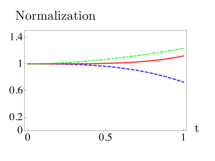
Figure 2: Normalization factor calculated for terms including only $\Phi_{0}(x)$ (dot-dashed line), $\Phi_{0}(x)$ and $\Phi_{2}(x)$ (dashed line) and $\Phi_{0}(x)$, $\Phi_{2}(x)$ and $\Phi_{3}(x)$ (solid line).

In this situation, it makes sense to introduce the “normalized Ansatz”, in which $\varphi(x,t)$ is approximated by the ratio $\nu_{N}(x,t)\equiv\varphi_{(N)}(x,t)/I_{N}(t)$, so that the correct normalization of the $N$th approximant is guaranteed for all $t$. In particular, this gives

$$\nu_{2}(x,t)=(x\bar{x})^{t}\,\frac{\Gamma(2+2t)}{\Gamma^{2}(1+t)}\frac{1-t^{2}\ln x\,\ln\bar{x}}{1-t^{2}\left[(H_{t}-H_{1+2t})^{2}-\psi_{1}(2+2t)\right]}\ .$$ (24)

As seen from this formula (and also from Fig.3), the initial flat function immediately (for whatever small positive $t$) evolves into a function vanishing at the end points with its shape dominated by the $(x\bar{x})^{t}$ factor.

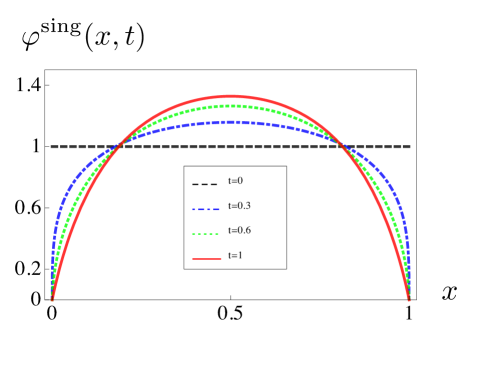
Figure 3: Evolution of the flat DA under the singular part of the evolution kernel: the curves shown correspond to $t=0,t=0.3,t=0.6,t=1.0$.

2.3 Adding Non-Singular Part

When the whole QCD evolution kernel is taken into account, we have

$$v(x)\equiv-\int_{0}^{1}[V(y,x)-V(x,y)]dy = 3/2+x\ln\bar{x}+\bar{x}\ln x$$

$$= v^{\text{sing}}(x)-1/2-x\ln x-\bar{x}\ln\bar{x}\ .$$

Following the same steps as in the previous section, we calculate the expansion terms for the initial flat distribution amplitude:

$$\Phi_{0}(x)= 1$$ (26)

$$\Phi_{1}(x)= 0$$ (27)

$$\Phi_{2}(x)= {x}\ln x+\bar{x}\ln\bar{x}+\frac{1}{2}x\ln^{2}x+\frac{1}{2}\bar{x}\ln^{2}\bar{x}+x\bar{x}\ln^{2}\frac{\bar{x}}{x}-\ln x\ln\bar{x}$$

$$+x\text{Li}_{2}\left(-\frac{\bar{x}}{x}\right)+\bar{x}\text{Li}_{2}\left(-\frac{x}{\bar{x}}\right)\ .$$ (28)

With these terms taken into account we have

$$\varphi_{(2)}(x,t) = e^{3t/2}\,(x^{\bar{x}}\bar{x}^{x})^{t}\left(1+\frac{t^{2}}{2!}\Phi_{2}(x)\right)\ .$$ (29)

Unfortunately, for this form it is impossible to analytically calculate the normalization integral even for the lowest term. Compared to the Ansatz used for the singular part of the evolution kernel, the Ansatz

$$\varphi(x,t)=e^{tv(x)}\Phi(x,t)=e^{3t/2}(x^{\bar{x}}\bar{x}^{x})^{t}\Phi(x,t)$$ (30)

has an extra overall factor $[e^{-1/2}x^{-x}\bar{x}^{-\bar{x}}]^{t}\ .$ Note that the function $x^{-x}\bar{x}^{-\bar{x}}$ is finite at the end points $x=0,\,1$, where it takes its minimal value for the interval $[0,1]$ (equal to 1), and has a maximum for $x=1/2$, where it equals 2. Thus, the factor $e^{-1/2}x^{-x}\bar{x}^{-\bar{x}}$ enhances the $x\bar{x}$ profile in the middle (by $2/\sqrt{e}\approx 1.2$ factor) and suppresses it at the end points (by $1/\sqrt{e}\approx 0.6$). This is a rather mild modification, and what is most important, it does not change the $\sim x^{t}$ (or $\sim\bar{x}^{t}$) behavior at the end points. So, it makes sense to use the expansion

$$[x^{-x}\bar{x}^{-\bar{x}}]^{t}=\sum_{n=0}^{\infty}(-1)^{n}(x\ln x+\bar{x}\ln\bar{x})^{n}\,\frac{t^{n}}{n!}\ ,$$ (31)

in powers of $t$ and combine it with the expansion for $\Phi(x,t)$. This corresponds to Ansatz

$$\varphi(x,t) = (x\bar{x})^{t}\,e^{3t/2}\,\left(\tilde{\Phi}_{0}(x)+t\,\tilde{\Phi}_{1}(x)+\frac{t^{2}}{2!}\tilde{\Phi}_{2}(x)+\ldots\right)\ ,$$ (32)

whose expansion coefficients $\tilde{\Phi}_{n}(x)$ can be straightforwardly obtained from $\Phi_{n}(x)$’s. In particular, $\tilde{\Phi}_{1}(x)=-(x\ln x+\bar{x}\ln\bar{x})$, and $\tilde{\Phi}_{2}(x)=\Phi_{2}(x)+(x\ln x+\bar{x}\ln\bar{x})^{2}$.

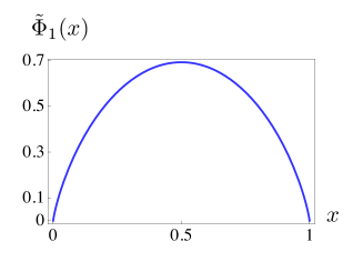
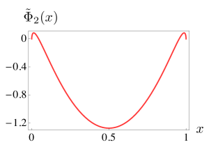
Figure 4: Expansion components in the full kernel case: $\tilde{\Phi}_{1}(x)$ (a) and $\tilde{\Phi}_{2}(x)$ (b).

Now, the normalization integral for the lowest terms can be calculated analytically:

$$I_{1}(t)\equiv\int_{0}^{1}\varphi_{(1)}(x,t)dx=e^{3t/2}\frac{\Gamma^{2}(1+t)}{\Gamma(2+2t)}\left(1-\frac{t}{2(t+1)}+\frac{t}{2}(-H_{t}+H_{1+2t})\right)\!,$$ (33)

where $H_{n}$ are harmonic numbers. Fig.5 shows the normalization versus $t$.

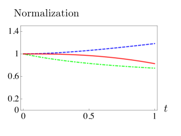
Figure 5: Same as in Fig.2 for the case of the full kernel.

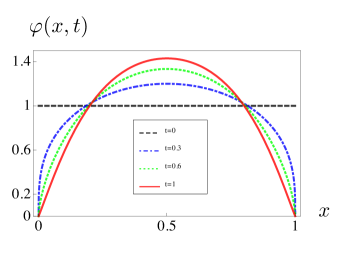
Figure 6: Same as in Fig.3 for the case of the full kernel.

Again, we may switch to the normalized Ansatz formed by the ratio $\varphi_{(N)}(x,t)/I_{N}(t)$. For a flat initial distribution, this gives

$$\nu_{1}(x,t)=(x\bar{x})^{t}\,\frac{\Gamma(2+2t)}{\Gamma^{2}(1+t)}\frac{1-t\,(x\ln x+\bar{x}\ln\bar{x})}{1-{t}/{2(t+1)}+{t}(-H_{t}+H_{1+2t})/2}\ .$$ (34)

The results are illustrated by Fig. 6.

3 Evolution of Anti-Symmetric Flat DA

3.1 Singular Part

Evolution equations may be applied also in situations when the distribution amplitude is antisymmetric with respect to the change $x\to 1-x$. An interesting example is the $D$-term function $d(x)$ that appears in generalized parton distributions. Thus, let us consider evolution of the DA that initially has the form

$$\varphi_{0}(x)=\begin{cases}\,\,\,\,1&0<x\leqslant 1/2\ ,\\ -1&1/2<x<1\ .\end{cases}$$

The $v(x)$ function (11) is the same, since it depends on the kernel only. Thus we can use the same Ansatz (6) and expansion (8). Since $\varphi_{0}(x)$ is not just a constant, the first expansion coefficient $\Phi_{1}(x)$ is nonzero. Let us start with the singular part of the kernel. Then we get

$$\Phi_{1}(x)=\begin{cases}-2\ln\left[\frac{\bar{x}}{1-2x}\right]&0<x\leqslant 1/2\ ,\\ \,\,\,\,\,2\ln\left[\frac{x}{-1+2x}\right]&1/2<x\leqslant 1\ .\end{cases}$$

We see that there are logarithmic terms $\ln|1-2x|$ singular for $x=1/2$. These terms are natural, since each half of the antisymmetric DA on its interval is expected to evolve similarly to a flat DA on the $0\leq x\leq 1$ interval. This observation suggests the Ansatz

$$\varphi(x,t)=e^{2t}(x\bar{x})^{t}|1-2x|^{2t}\Phi(x,t)\ .$$ (35)

With this definition of $\Phi(x,t)$, the $\ln|1-2x|$ terms are eliminated from $\Phi_{1}(x)$:

$$\Phi_{1}(x)=-2\ln\bar{x}\ \theta(0<x\leqslant 1/2)-\{x\to\bar{x}\}\ .$$ (36)

For the expansion component $\Phi_{2}(x)$, we have

$$\Phi_{2}(x)= \theta(0<x\leqslant 1/2)\Biggl{\{}-\frac{2\pi^{2}}{3}-2\ln\bar{x}\ln x-\ln^{2}(1-2x)-3\ln\bar{x}(\ln(x\bar{x})-1)$$

$$-2\ln(1-2x)(\ln(4\bar{x}x)+\ln(x\bar{x}))-8\text{Li}_{2}(1-2x)-4\text{Li}_{2}(x)-4\text{Li}_{2}(2x)$$

$$+2\text{Li}_{2}\left[\frac{x}{\bar{x}}\right]+4\text{Li}_{2}\left[\frac{x}{2x-1}\right]+4\text{Li}_{2}\left[\frac{1-2x}{\bar{x}}\right]\Biggr{\}}-\{x\to\bar{x}\}\ .$$ (37)

The graphical results for the expansion components are shown in Fig. 7.

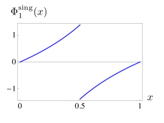
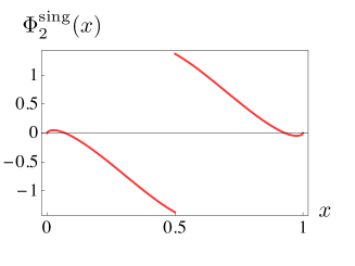
Figure 7: Expansion coefficients for the antisymmetric DA: $\Phi^{\text{sing}}_{1}(x)$ (a), $\Phi^{\text{sing}}_{2}(x)$ (b).

The evolution of $\varphi_{\text{sing}}(x,t)$ to this accuracy can be obtained from

$$\varphi(x,t)=e^{2t}(x\bar{x})^{t}|1-2x|^{2t}\left(\varphi_{0}(x)+t\Phi_{1}(x)+\frac{t^{2}}{2!}\Phi_{2}(x)\right).$$ (38)

As shown in Fig.8, the initial step function evolves into a function which is zero at the end points and in the middle point.

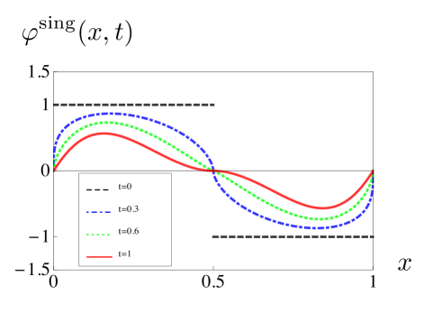
Figure 8: Evolution of antisymmetric DA under the singular part of the kernel for $t=0,t=0.3,$ $t=0.6,t=1$

3.2 Adding the Non-Singular Part

Since the nonsingular part does not add $\ln x$ and $\ln\bar{x}$ terms to $v(x)$, we may proceed with the same Ansatz

$$\varphi(x,t)= e^{3t/2}(x\bar{x})^{t}|1-2x|^{2t}\Phi(x,t)\,,$$ (39)

but the expansion components change (see Fig.9).

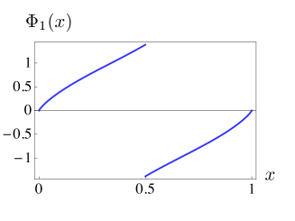
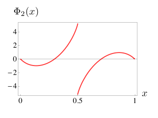
Figure 9: Expansion components $\Phi_{1}(x)$ (a) and $\Phi_{2}(x)$ (b) in the case of the full kernel.

The distribution amplitude is now built using

$$\varphi(x,t) = e^{3/2t}(x\bar{x})^{t}|1-2x|^{2t}\left(\varphi_{0}(x)+t\Phi_{1}(x)+\frac{t^{2}}{2!}\Phi_{2}(x)\right),$$ (40)

For the first coefficient we have

$$\Phi_{1}(x)=\theta(0<x\leqslant 1/2)\bigl{[}-2x\ln 2-2\ln\bar{x}-(\bar{x}\ln\bar{x}+x\ln x)\bigl{]}-\{x\to\bar{x}\}\ ,$$ (41)

and for the second,

$$\Phi_{2}(x)= \theta(0<x\leqslant 1/2)\Biggl{\{}\frac{\pi^{2}}{2}(x-2)+2\ln^{2}\left(\frac{\bar{x}}{1-2x}\right)+(3x-2)\ln^{2}2$$

$$+\left(\frac{13}{2}-3x\right)\ln^{2}\bar{x}+\ln(1-2x)(4(3-2x)\ln 2+2(5-2x)\ln x)$$

$$+\ln\bar{x}(1-2(1-3x)\ln 2+(3x-5)\ln x)+x\left(4\ln x\ln 2+\ln\left(\frac{4x}{\bar{x}}\right)\right)$$

$$-4\bar{x}\text{Li}_{2}\left(\frac{1-2x}{2\bar{x}}\right)-2(x-4)\text{Li}_{2}\left(\frac{1-2x}{\bar{x}}\right)-2(5+x)\text{Li}_{2}(x)$$

$$+2(5-2x)\text{Li}_{2}(2x)-(1+2x)\text{Li}_{2}\left(-\frac{x}{\bar{x}}\right)$$

$$+\text{Li}_{2}\left(\frac{x^{2}}{\bar{x}^{2}}\right)+4\text{Li}_{2}\left(-\frac{x}{1-2x}\right)\Biggl{\}}-\{x\to\bar{x}\}\ .$$ (42)

As may be seen from Fig.10, the resulting curves are rather close to those obtained when only singular part of the kernel was taken into account.

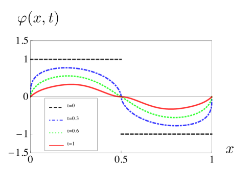
Figure 10: Evolution of the antisymmetric DA in the full kernel case. The curves for $t=0,$ $t=0.3,t=0.6,t=1$ are shown.

4 Summary

We described a new analytical method of performing ERBL evolution. Unlike the standard method of expansion in Gegenbauer polynomials, the method works for functions that do not vanish at the end points. The method was applied for two cases of the initial DA: for a purely flat DA, constant in the whole $0\leq x\leq 1$ interval and for an antisymmetric DA which is constant in each of its two parts $0\leq x\leq 1/2$ and $1/2\leq x\leq 1$. In case of a purely flat DA, the leading term gives $(x\bar{x})^{t}$ evolution with the change of the evolution parameter $t$. For the accompanying factor, two further terms in the $t^{N}$ expansion were found. In case of an antisymmetric flat DA, there is an extra factor $|1-2x|^{2t}$ that takes care of the jump in the middle point $x=1/2$. The correction terms were also calculated. The results show good convergence for $t\lesssim 1/2$. It should be noted that for $t\gtrsim 1/2$, the evolved DA is rather close to the asymptotic form, and one can use the standard method of the Gegenbauer expansion which is well convergent for such functions.

Notice: Authored by Jefferson Science Associates, LLC under U.S. DOE Contract No. DE-AC05-06OR23177. The U.S. Government retains a non-exclusive, paid-up, irrevocable, world-wide license to publish or reproduce this manuscript for U.S. Government purposes.

References

- [1] B. Aubert et al., Phys. Rev. D80, 052002 (2009).
- [2] G. P. Lepage and S. J. Brodsky, Phys. Rev. D22, 2157 (1980).
- [3] A. V. Radyushkin, Phys. Rev. D80, 094009 (2009).
- [4] M. V. Polyakov, JETP Lett. 90, 228 (2009).
- [5] A. V. Efremov and A. V. Radyushkin, Phys. Lett. B94, 245 (1980).
- [6] S. J. Brodsky, F.-G. Cao and G. F. de Teramond, arXiv:1104.3364 [hep-ph] (2011).
- [7] W. Broniowski, E. R. Arriola and K. Golec-Biernat, Phys. Rev. D77, 034023 (2008).
- [8] M. V. Polyakov and C. Weiss, Phys. Rev. D60, 114017 (1999).