Composition and evolution of Interstellar Grain mantle under the effects of photo-dissociation

Abstract

We study the chemical evolution of interstellar grain mantle by varying the physical parameters of the interstellar medium (ISM). To mimic the exact interstellar condition, gas grain interactions via accretion from the gas phase and desorption (thermal evaporation and photo-evaporation) from the grain surface are considered. We find that the chemical composition of the interstellar grain mantle is highly dependent on the physical parameters associated with a molecular cloud. Interstellar photons are seen to play an important role towards the growth and the structure of the interstellar grain mantle. We consider the effects of interstellar photons (photo-dissociation and photo-evaporation) in our simulation under various interstellar conditions. We notice that the effects of interstellar photons dominate around the region of lower visual extinction. These photons contribute significantly in the formation of the grain mantle. Energy of the incoming photon is attenuated by the absorption and scattering by the interstellar dust. Top most layers are mainly assumed to be affected by the incoming radiation. We have studied the effects of photo-dissociation by varying the number of layers which could be affected by it. Model calculations are carried out for the static (extinction parameter is changing with the density of the cloud) as well as the time dependent case (i.e., extinction parameter and number density of the cloud both are changing with time) and the results are discussed in details. Different routes to the formation of water molecules are studied and it is noticed that around the dense region, production of water molecules via O₃ and H₂O₂ contributes significantly. At the end, various observational evidences for the condensed phase species are summarized with their physical conditions and are compared with our simulation results.

1 Introduction

The densities in the interstellar space (consisting of 99% gas and 1% dust), even in the densest interstellar clouds, are so low that they are beyond the capabilities of the best vacuum systems on Earth. Even then, a large number of infrared absorption features are observed toward low and high mass protostars. Some of these features are attributed to the solid state interstellar molecules (Boogert & Ehrenfreund, 2004). Discovery of these interstellar molecules in condensed phase demands a proper explanation for the interstellar chemical composition budget. Increasing observational and experimental evidences in the gas phase points to the inadequacy of the gas phase chemistry and suggests the need to incorporate the grain surface processes. Interstellar dust grains are thought to be consisting of an amorphous silicate or carbonaceous core surrounded by a molecular ice layer (Draine et al.,, 2003; Gibb et al.,, 2004). Presently, very little is known about the morphology or chemistry on these grain surfaces, or the porosity of the grains themselves. Similarly, the chemical and physical processes on the grain surfaces till date are also very poorly known. A number of theoretical attempts have been carried out to verify the observed abundances of the gas phase and the condensed phase species (Hollenbach & Salpeter, 1970; Watson & Salpeter, 1972; Allen & Robinson, 1975; Tielens & Hagen, 1982; Hasegawa et al., 1992; Charnley, 2001; Stantcheva et al., 2002; Cuppen & Herbst, 2007; Chakrabarti et al., 2006a, b; Das et al., 2008a, b; Das et al.,, 2010). Both the deterministic and stochastic approaches are tested by these studies. Observational and experimental evidences suggest that almost 90% of the grain mantle is covered with H₂O, CH₃OH and CO₂. In our earlier paper Das et al., (2010), (hereafter DAC10), we mentioned that it is very difficult to theoretically match the exact observed abundances of all the three molecules simultaneously. Results of the numerical simulations show that only in a narrow region of parameter space all these three molecules are produced within the observed limit.

It is well known that the ISM chemistry is highly influenced by the interstellar UV radiations which mainly come from the nearby young stars. UV radiation affects the chemistry of the ISM through photo-dissociation and photo-ionization of the molecules and atoms. Several works are carried out to study the photo-chemistry in the ice containing simple as well as complex molecules. Most of the studies (Hagen et al., 1979; D’Hendecourt al., 1982; Allamandola et al., 1988) are concentrated following the irradiation of ice mixtures to reflect the chemical composition of the star forming regions. These types of studies give us an insight about the photo effects on the interstellar ice mantles.

Structure of the interstellar ices under various physical circumstances are yet to fully understood. Water ice is less abundant along some lines of sight. In the present paper, we carry out a coupled gas-grain study to fully understand the structure of the interstellar grain mantle around various lines of sight. Gas-grain interactions are considered via accretion from gas phase and evaporation from grain surface. Important surface reactions, which are feasible under the interstellar conditions are considered in our surface chemistry network to have clear insight of the interstellar ice feature. Moreover, to mimic the realistic situation, the formation of several mono-layers are considered. As we are interested only around the dense region of the molecular cloud, we assume that the major portion of the gas phase carbon atoms are already converted into carbon monoxide and as in the other models (Stantcheva et al., 2002; Das et al., 2008b; Das et al.,, 2010), we also consider the accretion of H, O and CO from the gas phase to follow the time evolution of several chemical species. Recent experimental findings of several new reaction pathways and several interaction energies involved during these process, motivate us to update our earlier DAC10 model. Our main aim in the present context is to study the formation of ice mantle under the influence of photo-processing and to make a comparative study among different routes to the water formation. This has been suggested recently by some experiments (Ioppolo et al.,, 2008). We also compare our simulation results with other observational, experimental and theoretical results carried out till date. In Section 2, we discuss the physical processes and the method used for the modeling. Extensive discussions along with the results are presented in Section 3. In Section 4, a comparison between the theoretical and observational results are presented. Finally, in Section 5 we have summarized our work.

2 Procedure

In general, the rate equation method (Hasegawa et al., 1992; Roberts & Herbst, 2002) is widely used to follow the surface process occurring under the interstellar condition. Main advantage of this method is that the computation is very fast. This method assumes the average concentration of species to follow the chemical evolution. Main drawback with this method is that it does not consider the statistical fluctuations and discrete nature of the species. As a result, this method is very much dependent on the physical conditions of the interstellar cloud. In the lower accretion rate regime, where surface population is comparatively lower, this method tends to overestimate the result (Chakrabarti et al., 2006a, b; Das et al., 2008b; Das et al.,, 2010). Moreover as this method deals with the average concentration, it is not able to follow the internal structure of the grain mantle. However, as the time passes by, grains are expected to grow in size with several surface species. As the rate equation is unable to trace any particular species, it is not possible for this method to mimic the actual situation in ISM. This is the reason, we use the descrete-time random walk Monte Carlo method to have more accurate results. In our approach, fluctuations in the surface abundance due to the statistical nature of the grain is preserved and as a result this method is much more realistic to study the interstellar surface chemistry. With this method, we can follow movements of each species and evaluate the results at every instant.

Details of the processes we follow are already discussed in Das et al., (2010). For the sake of completeness, we discuss them again briefly. We assume that the grains are square shaped and similar to an atom on an fcc[100] plane, each grain site has four nearest neighbors. We assume the periodic boundary conditions and also allow the possibility to form multiple layers on a grain surface. For modeling purposes, we consider classical dust grains, characterized by 1000A^∘ and 10⁶ surface sites. Following Hasegawa et al. (1992), we consider the surface density of available sites to be 1.5 $\times 10^{15}$ cm^-2. Number density of the grains are taken to be 1.33$\times 10^{-12}n$ ($n$ is the concentration of H nuclei in all forms) and gas to dust ratio is taken to be $100$ by mass(Hasegawa et al., 1992). Monte Carlo method is computationally much slower than the rate equation method and it is quite difficult to simulate for a grain having $10^{6}$ sites. To save computational time, we consider the grain having $50\times 50$ sites and the final results are extrapolated for the grain having $10^{6}$ sites. Reason behind choosing the grain having $50\times 50$ sites is that it is above the limit of the statistical fluctuating size and according to Chang et al. (2005), above this size, results are scalable and do not differ significantly. Location of the accreting species is dictated by generating a pair of random numbers. Langmuir Hinshelwood (reactions between the surface species via hopping) and Eley Rideal (reaction between the incoming species with the surface species), both types of reactions are considered. After landing on a grain, its direction towards any one of the four nearest neighbors is dictated by generating random numbers. Two possibilities may occur: If the site is occupied then either it will react when the reaction is permitted or it will wait until its next hopping time. If the neighboring site is vacant and it does not have any species just beneath that site then it can roll down on that grid until it touch some existing species in a layer or just the bare grain surface. If the reaction between the species touching the existing species is permitted, a new species is formed and if not, then it can sit on the top of that. For the reactions having barriers, we are generating random numbers upon each encounter and checking for the possibility of the reaction. Following Hasegawa et al. (1992) probability (P) for the reaction to happen upon an encounter is calculated and if the generated random number is less than P then the reaction is allowed and if the generated number is greater than P then reaction is discarded at that instant. Every species has its own hopping time scale. In our simulation, we consider the hopping time scale of H atom to be the minimum. After each interval of H hopping time, we are checking for the evaporation (via thermal or other process) and photo-dissociation by generating random numbers. For example, let us consider H₂O. Its evaporation rate is R_ev sec^-1. That means, one H₂O can evaporate after each $\frac{1}{R_{ev}}$ seconds of its formation on the grain. Since the smallest time scale is the hopping time scale $t_{H}$ of an H atom, after every $t_{H}$, we generate a random number to find out whether the species will evaporate or stick to the grain. If the generated number is smaller than $t_{H}\times R_{ev}$, then the species can evaporate. Photo-dissociations are also treated similarly, i.e., if the generated random number is under the probability of photo-dissociation of any species, that species can photo-dissociate. Gas phase compositions are adjusted at every $t_{H}$ after taking care of the accretion onto and the evaporation from the grains.

A major difference between our previous study and the present study is that we have updated our reaction network by considering several new reactions and have considered the effects of the cosmic rays as well. Cosmic rays have the direct/induced effect on the interstellar grain mantle. In our model, we consider the photo-dissociation and photo evaporation to incorporate the effects of the cosmic rays. Formation of the most abundant molecules such as, H₂O, CH₃OH and CO₂ are considered as before. Keeping in mind the recent experimental results (Ioppolo et al.,, 2008), we have also included the formation of H₂O via O₃ and H₂O₂ routes. All the reactions considered in our present model are given in Table 1. Activation barrier energy used in our previous paper (Das et al.,, 2010), and in some other papers (Stantcheva et al., 2002; Cuppen & Herbst, 2007) are noted in Tab.1. We gave some comments on the most recent experimental/theoretical findings in the last column. For the reaction numbers 4 and 6, we normally use $2000$K as the activation barrier energy (Stantcheva et al., 2002). However, the most recent findings by Fuchs et al., (2009), suggest that the energy barrier could be much lower ($390\pm 40$K for reaction number 4 and $415\pm 40$K for the reaction number 6 at $12$K). In our model calculation, we assume that at $10$K, the energy barrier is $390$K for the reaction number 4, and $415$K for the reaction number 6. So far, barrier energy $1200$K was used as mentioned in Melius & Blint (1979). Recent experimental findings by Ioppolo et al., (2008) suggest that the reaction number 12 is barrier less. Recent surface chemical modelling by Cazaux et al., (2010) assumed that the reaction number 14 is also barrier less though it is not experimentally verified. In our model, we assume reaction number 12 is barrier less and reaction number 14 with barrier 1400K (Klemm et al.,, 1975). Reaction number 16 is considered to have the activation energy $2600$K (Schiff, 1973). Binding energies of the species are the keys for the chemical enrichment of the interstellar grain mantles. Grain surface provides the space for the interstellar gas phase species to land on and to react with the other surface species. If allowed, chemical species can return back to the gas phase after chemical reactions or in the original accreted form. Reactions between the surface species is highly dependent on the mobility of the surface species, which in turn, depends on the thermal hopping time scale or on the tunneling time scale. For the lighter species, tunneling time scale is much shorter than the hopping time scale. So for the lighter species, surface migration by tunneling method might be effective. When two surface species meet, they can react. If some activation energy involved for that reaction to happen, they can react with a quantum mechanical tunneling probability (P). Goumans & Andersson (2010) studied the tunnelling reaction between O and CO with direct dynamics employing density functional theory and they obtained the activation energy 2500K for the reaction between O and CO. We use only thermal hopping of O atom for its mobility on the grain surface and use the same activation barrier energy, 2500K following Goumans & Andersson (2010) for the reaction number 9 of Tab. 1. In Das et al. (2008b), a comparative study between tunneling and hopping for the mobility of H atom on the grain surface was carried out and it was noticed that results did not show drastic variation within the accretion regime considered here (number density 10³-10⁶). We expect that as long as the accretion rate is within the limit , this does not significantly affect the final results.

There are two types of binding energies associated with the physical processes at low temperature, namely, physisorption and chemisorption. Among them, physisorption energies are more probable in low temperature ($\sim 10$K) condition, i.e., frigid (low temperature, $\sim$ 10K) condition. Therefore, in our model calculations, we considered the physisorption energies. We defined the whole system with a lot of interaction energies. Most of the energies considered here are discussed in detail in Das et al., (2010) and references therein. The rest of the species which are updated in our present model are given in Table 2. It is very difficult to find the exact binding energies for every specific surface. In Das et al., (2010), olivine surface was considered for the modeling purpose. Presently, we also considered olivine surface as a model substrate. Among the updated chemical species, binding energies of HO₂, O₃ and H₂O₂ are taken from Cazaux et al., (2010). They used the physisorbed energies of these molecules for the Carbonaceous grain and here we have included their values as if those are the interaction energies with the bare olivin surfaces. For C atom, we used the same binding energy as in CO. For CH₃ and CH₂OH, we used the same binding energies as in CH₃OH and H₂CO respectively. Since the binding energies of these species are very high, we can be sure that our assumptions would not alter the final results significantly. Due to the lack of knowledge of the appropriate interaction energies between various species, we assumed that the binding energies of these species with other surface species are the same as with olivine surfaces.

Table 1: Surface Reactions considered in our network

	Reactions	Ea(K)	Comments
1	H+H $\rightarrow$ H2
2	H+O $\rightarrow$ OH
3	H+OH $\rightarrow$ H2O
4	H+CO $\rightarrow$ HCO	2000	390K $\pm$ 40K at 12K (Fuchs et al.,, 2009)
5	H+HCO $\rightarrow$ H2CO
6	H+H2CO $\rightarrow$ H3CO	2000	415K $\pm$ 40K at 12K (Fuchs et al.,, 2009)
7	H+H3CO $\rightarrow$ CH3OH
8	O+O $\rightarrow$ O2
9	O+CO $\rightarrow$ CO2	1000	2970K (Talbi et al., 2002), 2500K (Goumans & Andersson, 2010)
10	O+HCO $\rightarrow$ CO2+H
11	O+O${}_{2}\rightarrow$ O3
12	H+O${}_{2}\rightarrow$HO2	1200	barrier less (Ioppolo et al.,, 2008)
13	H+HO${}_{2}\rightarrow$H2O2
14	H+H2O${}_{2}\rightarrow$H2O+OH	1400	barrier less (Cazaux et al.,, 2010)
15	H+O${}_{3}\rightarrow$ O2+OH	450
16	H2+OH$\rightarrow$ H2O+H	2600

Table 2: Energy barriers in degree Kelvin

Species	Substrate
	Silicate	H	$\bf{\mathrm{H_{2}}}$	O	$\bf{\mathrm{O_{2}}}$	OH	$\bf{\mathrm{H_{2}O}}$	CO	HCO	$\bf{\mathrm{H_{2}CO}}$	$\bf{\mathrm{H_{3}CO}}$	$\bf{\mathrm{CH_{3}OH}}$	$\bf{\mathrm{CO_{2}}}$	$\bf{\mathrm{HO_{2}}}$	$\bf{\mathrm{H_{2}O_{2}}}$	$\mathrm{O_{3}}$	$\mathrm{C}$	$\mathrm{CH_{3}}$	$\mathrm{CH_{2}OH}$
H	350	350	45	350	45	350	650	350	350	350	350	350	350	350	350	350	350	350	350
$\mathrm{H_{2}}$	450	30	23	30	30	30	440	450	450	450	450	450	450	450	450	450	450	450	450
O	800	480	55	480	55	55	800	480	480	480	480	480	480	800	800	800	800	800	800
$\mathrm{O_{2}}$	1210	69	69	69	69	1000	1210	1210	1210	1210	1210	1210	1210	1210	1210	1210	1210	1210	1210
OH	1260	1260	240	240	240	240	3500	1260	1260	1260	1260	1260	1260	1260	1260	1260	1260	1260	1260
$\mathrm{H_{2}O}$	1860	390	390	390	390	390	5640	1860	1860	1860	1860	1860	1860	1860	1860	1860	1860	1860	1860
CO	1210	1210	1210	1210	1210	1210	1210	1210	1210	1210	1210	1210	1210	1210	1210	1210	1210	1210	1210
HCO	1510	1510	1510	1510	1510	1510	1510	1510	1510	1510	1510	1510	1510	1510	1510	1510	1510	1510	1510
$\mathrm{H_{2}CO}$	1760	1760	1760	1760	1760	1760	1760	1760	1760	1760	1760	1760	1760	1760	1760	1760	1760	1760	1760
$\mathrm{H_{3}CO}$	2170	2170	2170	2170	2170	2170	2170	2170	2170	2170	2170	2170	2170	2170	2170	2170	2170	2170	2170
$\mathrm{CH_{3}OH}$	2060	2060	2060	2060	2060	2060	2060	2060	2060	2060	2060	2060	2060	2060	2060	2060	2060	2060	2060
$\mathrm{CO_{2}}$	2500	2500	2500	2500	2500	2500	2500	2500	2500	2500	2500	2500	2500	2500	2500	2500	2500	2500	2500
$\mathrm{HO_{2}}$	2160	2160	2160	2160	2160	2160	2160	2160	2160	2160	2160	2160	2160	2160	2160	2160	2160	2160	2160
$\mathrm{H_{2}O_{2}}$	2240	2240	2240	2240	2240	2240	2240	2240	2240	2240	2240	2240	2240	2240	2240	2240	2240	2240	2240
$\mathrm{O_{3}}$	2900	2900	2900	2900	2900	2900	2900	2900	2900	2900	2900	2900	2900	2900	2900	2900	2900	2900	2900
$\mathrm{C}$	1210	1210	1210	1210	1210	1210	1210	1210	1210	1210	1210	1210	1210	1210	1210	1210	1210	1210	1210
$\mathrm{CH_{3}}$	2060	2060	2060	2060	2060	2060	2060	2060	2060	2060	2060	2060	2060	2060	2060	2060	2060	2060	2060
$\mathrm{CH_{2}OH}$	1760	1760	1760	1760	1760	1760	1760	1760	1760	1760	1760	1760	1760	1760	1760	1760	1760	1760	1760

For the all species $E_{b}=0.3\ E_{D}$ is used except the atomic hydrogen where $E_{b}=0.2857\ E_{D}$ is used. For the reference please see the text.

Table 3: Interstellar photo reactions considered at the present work.

		Cosmic ray induced rates (Ri)			Direct cosmic ray rates (Rd)
	Reactions	$\alpha$	$\beta$	$\gamma$	$\alpha$	$\beta$	$\gamma$
1	aO${}_{2}\rightarrow$ O+O	1.0(-16)	0(0)	3.755(2)	1.90(-9)	0(0)	1.85(0)
2	aOH$\rightarrow$ O+H	1.0(-16)	0(0)	2.545(2)	3.90(-10)	0(0)	2.24(0)
3	H2O$\rightarrow$ H+OH	1.3(-17)	0(0)	4.855(2)	5.90(-10)	0(0)	1.70(0)
4	CO$\rightarrow$ C+O	1.3(-17)	0(0)	1.050(2)	2.00(-10)	0(0)	2.50(0)
5	HCO$\rightarrow$ H+CO	1.3(-17)	0(0)	2.105(2)	1.10(-9)	0(0)	8.0(-1)
6	H2CO$\rightarrow$ H2+CO	1.3(-17)	0(0)	1.329(3)	7.00(-10)	0(0)	1.7(0)
7	CH3OH$\rightarrow$ CH3+OH	1.3(-17)	0(0)	7.520(2)	6.00(-10)	0(0)	1.8(0)
8	CO2$\rightarrow$ CO+O	1.3(-17)	0(0)	8.540(2)	1.40(-9)	0(0)	2.50(0)
9	H2O2$\rightarrow$ OH+OH	1.3(-17)	0(0)	7.500(2)	5.90(-10)	0(0)	1.7(0)
10	aO3$\rightarrow$ O2+O	1.0(-16)	0(0)	3.755(2)	1.95(-9)	0(0)	1.85(0)
11	aHO2$\rightarrow$ OH+O	1.0(-16)	0(0)	3.750(2)	6.70(-9)	0(0)	2.12(0)

All rates are taken from Woodall et al., (2007) except the reactions denoted by ^a (Cazaux et al.,, 2010).

3 Results & Discussion

3.1 Effect of photo dissociation

Photo-dissociation of the interstellar grain mantle plays an important role in the evolution of the interstellar grain mantle. This feature is included in our present model. Due to the lack of knowledge about the different photo-dissociation rates of the surface species, we assumed that the photo-dissociation rates of the surface species are the same as in the gas phase species. List of photo reactions along with the various parameters necessary for the direct cosmic ray photo reactions and cosmic ray induced photo reactions are noted in Table 3. Reactions which are taken from Woodall et al., (2007), rates are calculated by;

$$R_{i}=\alpha(\frac{T}{300})^{\beta}\frac{\gamma}{1-\omega}\ \ s^{-1},$$ (1)

where, $\alpha\ ,\ \beta\ ,\ \gamma$ are three constants, $T$ is the grain temperature, $\omega$ is the dust grain albedo in far ultra-violet. Here we use $\omega=0.6$ in our all calculations. For the other Cosmic ray induced photo reactions which are marked by ‘^a’ in Table 3, we calculate the rate by the following equation;

$$R_{i}=\alpha\gamma.$$ (2)

For the direct interstellar photo reactions, the rate is derived as;

$$R_{d}=\alpha exp(-\gamma A_{v})\ \ s^{-1},$$ (3)

where, $A_{v}$ is the extinction at visible wavelengths caused by the interstellar dust.

Normally, first few layers are assumed to be affected by the interstellar photons. Keeping this in mind, we use Monte-Carlo approach to investigate this aspect. Probabilities of photo reactions and photo evaporations are applied by the use of random number generators. After the photo dissociation, the heavier counterpart is allowed to replace the dissociated species and the comparatively lighter counterpart is stored in the nearby vacant sites or react with other nearby suitable species of the same layer. If there are no site available on the same layer to satisfy the criterion, dissociated lighter species may drop down to the lower vacant site or act with some other suitable reactant. After this, if it fails to find out a suitable location then the lighter species is allowed to evaporate. We notice that during our simulation time scale, the evaporation probability of the lighter counterpart is close to zero, so this assumption should not result in any error. Photo-evaporation are also incorporated in our code by the help of the random number generator as discussed earlier.

Mobility of a species inside the ice leads to chemical enrichment of the interstellar grain mantle. Photo-dissociation adds up a new dimension to the ice mantle by changing its morphology. Its contribution towards the final structure of the interstellar grain mantle should not be neglected around some regions of the ISM.

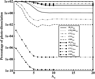
Figure 1: Variation of percentage of photo-dissociation as a function of the extinction parameter A_V. Results obtained by Monte-Carlo simulations are found to be consistently lower compared to those obtained from rate equations.

3.1.1 Dependence on the Extinction parameter

In Fig. 1, percentage of photo-dissociated molecules are plotted with the extinction parameter. Both the Rate equation and Monte Carlo methods are considered for a thorough study of these effects. Along the ‘Y’ axis we have shown the percentage of molecules which are photo-dissociated for a given species. For the better agreement of our simulated results with the observations, we choose the initial conditions around the favorable zone mentioned in DAC10 (Das et al.,, 2010). DAC10 parameters consist of hydrogen number density ($\sim 10^{4}$ cm^-3), atomic Hydrogen number density ($\sim 1.10$ cm^-3), atomic Oxygen number density ($\sim 1.05$ cm^-3), Carbon-monoxide number density ($0.375$ cm^-3), and temperature ($10$K). Unless otherwise stated, throughout the paper we use the DAC10 parameters as the initial condition and all the results are shown after evolving the system up to two million years. For the regions having other number densities, we scale the number density of O and CO accordingly by keeping the atomic hydrogen number density of $1.10$ cm^-3. It is evident from Fig. 1 that the lower extinction regions are heavily affected by the interstellar photons. For this simulation, we assume that only first mono-layer of the evolving grain mantle is exposed to the interstellar gas and photo-reaction/evaporation can only occur from the first mono-layer.

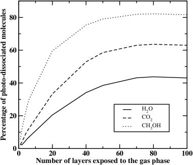
Figure 2: Effect of photo-dissociation on the number of layers exposed to the gas phase. Note that beyond fifty mono-layers, there is a saturation in photo-dissociation.

It is clear from the figure that in the Monte Carlo method, the water (1%-98%), methanol (6%-95%) and CO₂ (91%-99%) production is heavily influenced due to interstellar photons and the effects are prominent. Photo-dissociations of CO ($0.07\%$-97$\%$) and OH ($0.009\%-42\%$) are significant in the Monte Carlo method at the lower extinction region. Around A${}_{V}=3$, the percentage of photo-dissociation of CO and OH are $2.3\%$ and $0.19\%$ respectively which turns into $97\%$ and $42\%$ respectively when $A_{v}=0.5$. This demonstrates how strongly the grain surface species are affected by the interstellar UV radiation field around the low extinction region.

In the Rate equation method, the trend is more or less similar. However, it is to be noted that the stable species are photo-dissociated in the Rate equation method more strongly as compared to the Monte Carlo method. OH and CO are comparatively less affected. The reason behind the enhanced photo-dissociation effect for the stable species in case of the Rate equation method is that this method is not capable of tracing the species layer wise or location wise. Hence the molecules are dissociated with a constant fraction always. However, for the Monte Carlo method, since we are considering the photo effect responsible for the first layer only, its contribution is lower than the Rate equation method. In the case of Rate equation method, trace amount of OH or CO is left over due to the formation of water but in case of Monte Carlo method, some OH may be sustained due to not having the suitable reactant partner or due to the ‘blocking effect’ For instance, if a reactive species is surrounded by various surface species with which reactions are not allowed or require high activation barrier energies, the species remains locked in until its desorption. If it overcomes the energy barrier during its lifetime on the grain or by any other mechanism such as evaporation or hopping of the surrounding species to free its location, then only the reactive species is unblocked. This is the ‘blocking effect’ and it is a very common feature around the dense cloud, where the surface species are very much abundant. Due to this reason, in the Monte Carlo method there are some OH or CO which are photo-dissociated as they remain in the grain for some time. On the contrary, in the case of Rate equation method this is not possible due to the production of molecules at a constant rate.

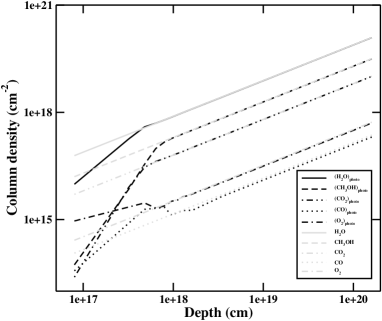
Figure 3: Column density of various species as a function of the distance inside the cloud measured from the surface. A comparison between the consideration of with and without the photo effects is shown.

3.1.2 Effects of the choice of the exposed layers

Interstellar radiation field is attenuated by the dust particles and thus the effects are also reduced with depth. The incoming particles have the energies in the range of $20-70$MeV nucleon^-1 which can deposit energy up to $0.4$ MeV (Leger et al.,, 1985) on an average into the classical size dust particles having radius $\sim 0.1$ $\mu$m. Several models are present to explain the interaction of interstellar energetic particles with the dust. Depending on the energy of the interacting particle, it can penetrate deep inside the grain mantle. Recent chemical model by Andersson et al., (2006) considered photo-dissociation of the top six layers only. Nguyen et al., (2002) assumed a limit of one hundred mono-layers that could be reached by photo-dissociation. Westley et al., (1995) assumed that most of the desorption takes place only from the outermost mono-layers. In Fig. 2, we have explained how the final results are altered by the assumption of the number of exposed layers to the gas phase. In all the cases Photo-desorption is asumed to be effective only from the top most layer and photo-dissociation is assumed to be effective upon the choice of the exposed layers. Along X-axis, we plot the choice of the number of upper layers which can be affected by the inter-stellar photon. Along Y-axis, we plot the percentage of photo-dissociated species at the end of the simulation time ($2\times 10^{6}$ year). Percentage is calculated by just calculating the ratio of total number of photo-dissociated H₂O, CO₂ or CH₃OH molecules with the total number of H₂O, CO₂ or CH₃OH produced during the simulation and multiplying the ratio by $100$. The life time of a molecular cloud is in general few million years. We restricted our simulation time up to 2 $\times$ 10⁶ year. In Fig. 2, results are presented for the intermediate density (10⁴ cm^-3) cloud after 2 $\times 10^{6}$ year, a steady state of the grain surface species is reached due to the depletion of the gas phase species by that time. As the gas phase composition changes, production of stable molecules are becoming less significant on the grain but the photodissociation rate is not changing. As a results, percentage of photo-dissociated molecules are dependent on the simulation time. But, since we are presenting the results at the end of the life time of the molecular cloud, in that sense results showing the final percentage of the photo-dissociated molecules.

As expected, the percentage of photo-dissociated molecules increases as the number of exposed layers increases. Mantle thickness grows up to $\sim 80-85$ layers for the physical conditions considered here. This calculation is carried out assuming the DAC10 parameters as the initial condition. Results are plotted after evolving the system up to two million years. After sixty layers the effects are slowed down. For the higher density region, where mantle grows up to several mono-layers these effects should be more enhanced. But one point should be remembered that in this case, the field strength itself will be attenuated, as it go deep inside the mantle and the effects might be visible for the top-most mono-layers only.

In our work, we have tested how the choices of number of exposed layers may affect the final results. Because the mantle column density is very low, we assumed that all the exposed layers, considered in the respective simulations, may ‘feel’ the effects of interstellar photons in a similar manner. In principle, it should have been decreased as it is going deep inside the mantle, but this may be negligible. In the rest of the paper, we consider two extreme cases: When the photo-dissociation is effective only for (a) the outermost layer and (b) uppermost fifty layers.

3.1.3 Column density

When we study molecular abundances, we do not see any local molecular density, but we observe only the column densities of the molecules. So theoretical calculation of the column density of a given molecule should be done in order to compare the theoretical and observational results. The column density of a species is given by (Shalabiea et al., (1994)),

$$N(A)=\Sigma n_{i}(A,R_{i})\Delta R_{i},$$ (4)

where, n_i(A,R_i) is the local number density of species $A$ at location $R_{i}$ and $\Delta R_{i}=R_{i}-R_{i-1}$ is the grid spacing along the radial($R$) direction. Number density of the species at the location $R_{i}$ is given by, $x_{i}=\frac{n_{i}(A,R_{i})}{{n_{H}}_{i}}$, where ${n_{H}}_{i}$ is the number density of the cloud at the $i^{th}$ location. Following Shalabiea et al., (1994), length of the line of sight R_tot can be represented as;

$$R_{tot}=\frac{1.6\times 10^{21}\times A_{v}}{{n_{H}}_{i}}\ {\rm cm},$$ (5)

where, A_V is the visual extinction of cloud. Taking summation over the entire grid (total $k$ number of grids),

$$\Sigma_{1}^{k}x_{i}=\Sigma_{1}^{k}\frac{n_{i}(A,R_{i})}{{n_{H}}_{i}}.$$ (6)

So the column density of a species ‘A’ is given by,

$$N(A)=\Sigma_{i}^{k}{n_{H}}_{i}x_{i}\Delta R_{i}.$$ (7)

For the constant density cloud, ${n_{H}}_{i}={n_{H}}$. We get,

$$N(A)=n_{H}\Sigma_{i}^{k}x_{i}\Delta R_{i}.$$ (8)

For $k=1$;

$$N(A)=n_{H}x_{i}\Delta R_{i}.$$ (9)

Thus, by knowing the extinction parameter, we can calculate the depth of a cloud from Eqn. 5 and the corresponding Column density from Eqn. 9. In Fig. 3, we show the depth dependence of the column density of the major interstellar grain surface species with and without interstellar photo effects. We assumed the initial conditions as in DAC10. From Fig. 3, it is clear that the column density increases with the depth of the cloud (measured from the outer edge), which indicates that as we are going deeper inside the cloud, production enhances. Pictures should be better interpreted if we assume that the extinction parameter consists of two components: the first one is $\leq$ 5 (corresponding depth $8\times 10^{17}$ cm, from Eqn. 9) and the next one is $\geq$ 5. For this figure, we have converted the final abundances into the column density after $2\times 10^{6}$ years. Low value of the extinction parameter means diffuse or weakly translucent cloud, so it is likely to evolve the cloud with much longer time (around $10^{7}$ years, here we evolve the cloud only up to $2\times 10^{6}$ year). In this lower region, we find out a very stiff slope of the column density with the extinction parameter/depth of the cloud, whereas at the moderate translucent cloud region ($A_{v}\geq 5$) we have almost a linear relationship. For the lower end of the extinction parameter or equivalently when length of the line of sight is smaller, we still have a significant water formation during the life time ($2\times 10^{6}$ year) of the molecular cloud. According to Murakawa et al., (2000), the observed column density of the condensed water molecules along the lower edge of the extinction parameter $\sim$ 0.5 is around $10^{17}$ cm ^-2. Murakawa et al., (2000) studied the Heiles Cloud 2, which is a part of the Taurus molecular cloud complex. Average number density of the dense core is around 10⁴ cm^-3 (Onishi et al.,, 1996). From Fig. 3, our calculated column density of condensed phase water is around $1.1\times 10^{16}$ cm^-2. For the lower extinction region, cloud may have larger life time, which means that we need to calculate the column density after much longer time than the previous cases. For the sake of completeness, we tested a case for $A_{v}=0.5$ (corresponds to the depth of $8\times 10^{16}$ cm) for 10⁷ years and obtain the column density of water ice around $4.6\times$ 10¹⁶cm^-2. This is much better than the previous estimate. Photo effect can be better understood if we make a comparison of two cases. In one case we include this effect, and in the other case we exclude this effect. In Fig. 3, gray lines are drawn for the cases where we have not considered the photo effects. Difference between the two results are distinctly visible towards the low extinction region. For the better realization of these differences, we have tabulated the column densities of the different species at Table 4 for A${}_{V}=0.5$ (corresponding depth 8$\times 10^{16}$ cm), which is the lowest value of the extinction used in this present paper. It is clear from the Table 4 that in the region of very low extinction, composition of the grain mantle is completely different due to the interstellar photo effect. Column densities of water & methanol are strongly affected by the interstellar photo reactions. Column densities of all the species are decreased except O₂. Interestingly, it is increasing around these region. The reason behind this increased column density of O₂ is that it can be easily photo-dissociated by forming two Oxygen atoms, which in turn react to form O₂ molecules again. Source of atomic oxygen may also come from the photo-dissociation of OH, CO₂, HO₂, O₃ and CO. Due to the large number of O atoms on the grain surfaces, O₂ abundances increased (Fig. 3).

Table 4: Effect of photo-dissociation for A${}_{V}=0.5$

Species	No photo effect	With photo effect
H2O	6.1 $\times 10^{16}$	1.1$\times 10^{16}$
CH3OH	1.6 $\times 10^{16}$	5.4$\times 10^{13}$
CO2	5.1 $\times 10^{15}$	3.3$\times 10^{14}$
CO	1.2$\times 10^{14}$	2.1$\times 10^{13}$
O2	2.7 $\times 10^{14}$	1$\times 10^{15}$

3.1.4 Relation between $A_{v}$ and hydrogen number density

Following Lee et al., (1996), the relationship between hydrogen density and visual extinction is given by,

$$n_{H}={n_{H}}_{0}[1+[{(\frac{{n_{H}}_{max}}{{n_{H}}_{0}})}^{1/2}-1)\frac{A_{v}}{{A_{v}}_{max}}]]^{2},$$ (10)

where, $n_{H}=n(H)+2n(H_{2}$) is the total hydrogen density in the unit of cm^-3, n${{}_{H}}_{0}$ is the cloud density at the cloud surface, n_Hmax is the maximum density and A${}_{V}{{}_{max}}$ is the maximum visual extinction considered very deep inside the cloud. Lee et al., (1996) considered the above relations for $T=30$K and here for the limitation of our present model we assume that this relation is valid for $10$K also. We assume that at the lowest depth (i.e., at the cloud surface) hydrogen density $n{{}_{H}}_{0}$ is $10^{3}\ cm^{-3}$ and it reaches its maximum $n{{}_{H}}_{max}=10^{5}\ cm^{-3}$ at deep inside the cloud (corresponding $A{{}_{V}}_{max}=150$). Composition of the gas phase around different regions are taken accordingly by just appropriate scaling of the DAC10 parameters. In Fig. 4, variation of column density with respect to the extinction parameters are shown. Column density of the species at different interstellar extinction is taken from results obtained at $2$ million years. The inset shows the variation of the number density for the varying extinction parameters. As in Fig. 3, here also H₂O is the major constituent of the grain mantle. Methanol is the $2^{nd}$ abundant contributor initially but deep inside the cloud its contribution slightly decreases. The reason behind is that due to the increasing number density around the region of high extinction parameters, accretion rates of O and CO increase and as a result, the surface coverage of O related species increases (CO₂ and O₂ increases). The accretion rate of atomic hydrogen is not increasing as we assumed that it is constant ($1.10$ cm^-3) around the all region, though in principle, it should have decreased slightly around the high density region. Due to the lack of atomic hydrogen on the grain surfaces, all the hydrogenated species are looking to be produced less efficiently around the high density/high extinction region. As a result, the surface coverage of CO increases rapidly around these regions.

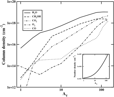
Figure 4: Variation of the column density with the extinction parameter. Inset shows the variation of density with the change of the extinction parameter.

3.1.5 Time dependent Case

Armed with various parameters, we will now simulate more realistic case, where the density is not constant with time. To start with, we assume that a cloud is collapsing from a low density region ($n{{}_{H}}_{0}=10^{3}$  cm^-3) to the higher density ($n{{}_{H}}_{max}=$10${}^{5}\ cm^{-3}$) region. Density is assumed to be increasing linearly with time and reaches its maximum at around $2$ million years. We assume that around the high density region, the cloud has the maximum value of the extinction parameter (${A_{v}}_{max}=150$) and the cloud is assumed to be collapsing isothermally ($T=10$K). Using Eqn. 10, we can calculate the corresponding extinction parameter. So in that way we now have a pseudo dynamic nature of the interstellar collapsing cloud where we have a relation between the time and the other parameters. The gas phase composition changes according to the density of the surrounding molecular cloud. The initial compositions are taken by appropriate scaling of the DAC10 parameters and effects of interstellar photons are considered only for the uppermost layer. Interaction of the gas and the grain are considered by assuming the accretion and evaporation process. Fig. 5 shows the time variations of column densities. Column density of species at a particular instant is calculated by just converting the abundance by Eqn. 9. It is evident from the figure that at the beginning, since the density is pretty low and the extinction is much lower, the longevity of the several species are restricted due to the strong radiation field. Inset pictures show the variation of the (a) hydrogen number density and the (b) extinction parameter with the time. At the beginning, due to the strong UV radiation field (low extinction parameter), the column density of several species fluctuates. After 10⁵ years, variations are more or less smoother due to the decrease in the radiation field in the high extinction parameter region. As like the other cases, here also water is the most abundant species. Surface coverage of methanol is noticed to be reduced heavily in compare to the other results.

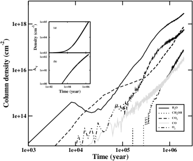
Figure 5: Time evolution of several condensed phase species are shown. Insets show the (a) time variation of density and the (b) time variation of the extinction parameter.

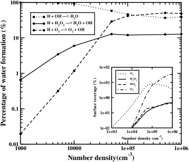
Figure 6: Different routes to H₂O.

3.2 Different routes to water formation

Recent experiment by Ioppolo et al., (2008) shows that there are alternative routes for the formation of water on the interstellar grain other than the traditional one (H+OH $\rightarrow$ H₂O). We have visited the problem of the water production via different routes by using our modified Monte Carlo code. Fig. 6 shows that the water molecules are mainly formed by the well known traditional route but as the density of the molecular cloud changes (for simplicity, we keep other physical constraints as constant: $A_{v}=10$ and $T=10$K), other pathways for the formation of water molecules also appears to be significant. For example, at lower density regions ($n\sim 10^{3}cm^{-3}$), almost 100% of the water molecules are formed by the traditional route but when the number density of hydrogen is around $10^{6}\ cm^{-3}$, this goes down to 39%. At higher number density regions, production of O₂ is favorable and due to the high surface coverage of solid O₂, O₃ can be produced very efficiently. Since the activation barrier energy for the reaction between H and O₃ is very low ($450$K), O₃ can readily react with H to form an OH, which in turn, form H₂O by another hydrogenation reaction. Formation of H₂O by the O₃ route is very efficient at high density regions (maximum $\sim 48\%$) compare to the low density region (around $\sim 0.02\%$). There is another route to H₂O, namely from H₂O₂. Reaction Nos. 12 to 14 are associated with the formation of H₂O via this route. Formation is maximum around the high density region (13%). At around $n\sim 10^{6}$ cm^-3, production of O₃ is highly favorable due to high surface coverage of atomic oxygen as well as O₂ molecules. O₃ molecules are produced efficiently via Langmuir Hinshelwood or via Eley Rideal method, as a result, the surface coverage of O₂ decreases. The inset clearly displays the above aspects showing the variation of the surface coverage of several condensed phase species with the number density of the molecular cloud. It is clear that the surface coverage of O₂ having a peak at around 10⁵ cm^-3 region and beyond this region as the density increases, rate of production of O₃ enhances. As a result, the surface coverage of O₂ decreases.

Around the dense region of the molecular cloud, H₂ is the most abundant species in the gas phase and H₂O can be very efficiently produced in the gas phase via reaction number 16 of Tab. 1. But the problem with H₂ is that it can not able to stick well with the grain surface (Leitch & Williams, 1985). So we use sticking coefficient of H₂ to be zero. As like the stantcheva 2002, Das et al., 2008b, and Das et al., 2010, here also we consider only the accretion of H, O and CO from the gas phase. In our model, we allow gas phase H₂ to react with surface OH via Eley-Rideal mechanism. But, as H₂ + OH reaction requires very high activation energy (2600K) Schiff (1973) and surface abundance of OH is very low, production of water via this route is negligible. H₂ may produce on the grain surface via reaction between two H atom and can contribute to the water formation route. But if we look at the accretion time scale of H atom onto a 50$\times$50 grain kept at T$\sim$10K, it comes out to be around $4.8\times 10^{7}$ sec for 10⁴ cm^-3 number density cloud. The evaporation time scale at 10K is around 535 sec. So there is no chance for one H to meet with other H via accretion. Despite of this fact H₂ may produce on the grain surface when two H atom meet together. For that instant one H is the accreted H atom and the second one is the product due to the reaction between O and HCO (reaction number 10 of Tab.1). Since the production of H₂ by this way also not significant enough, this reaction does not significantly contributes to the water formation on the grain.

3.3 Comparison with Observations and other Models

NGC 7538 IRS 9, W33A, W3 IRS 5, S140 IRS 1, RAFGL 7009S were chosen to compare our results with observations. The reasons behind choosing these sources are that these sources are believed to be protostellar objects which are deeply embedded inside dense molecular clouds. Beside this, they have a very high level of extinction from dust in the dense molecular cloud and they exhibit infrared spectra with the molecular ice feature. In Table 5, observed column densities as well as relative abundances of abundant observed ice species (H₂O, CH₃OH, CO₂, CO and O₂) along different lines of sight are compared with our various modeling results. Column densities are expressed in the unit of 10¹⁷ cm^-2. Normally relative abundances of ice species are used to express the observed ice features and this is calculated by just calculating the surface abundance of any species with respect to the surface abundance of water and then multiplying the factor by 100. Observed relative abundances along various sources as well as the relative abundances obtained from our simulation results are noted inside the bracket. Appropriate references for the observed data are noted at the bottom of the table. For the comparison purpose, four models are considered; DAC10a, DAC10b, DAC10a(m) and DAC10b(m). In DAC10a and DAC10b model, initial conditions are taken around the favourable zone of the parameter space (Das et al.,, 2010), having number density of the cloud 10⁴ cm^-3 and temperature 10K. Difference between DAC10a and DAC10b model is that, for DAC10a model, effect of photo reactions/evaporations are considered only for the outermost layer and for DAC10b model, Photo-dissociation is considered for the uppermost 50 layers but photo-evaporation is restricted only from the topmost layer. In DAC10a and DAC10b model, extinction parameter is assumed to be independent upon the initial number density of the cloud. In DAC10a(m) and DAC10b(m) model, density variation of the extinction parameters are taken into account (Eqn. 10). In the inset picture of Fig. 4, variation of number density with respect to the extinction parameter of the cloud is shown. These models may be better understood by just referring the section 3.1.4. Difference between DAC10a(m) and DAC10b(m) model is the same as the difference between the DAC10a and DAC10b model mentioned just above. Column densities from our simulation results are tabulated after two million years. Column density is calculated by using Eqn. 9, where column density is directly proportional to the extinction parameter (A_V). While we are considering the effect of photo-reactions for the uppermost 50 layers (DAC10b and DAC10b(m) model), production of the stable species(H₂O, CO₂, CH₃OH and O₂) decreases for most of the cases compare to the cases, where only topmost layer is considered for the effective photo reactions/evaporations (DAC10a and DAC10a(m) model). Opposite trend is noticed for the CO molecule. Since in case of DAC10b and DAC10b(m) model, a large number of CO₂ molecules can be affected by photodissociations (CO₂ $\rightarrow$ CO +O) compare to the DAC10a and DAC10a(m) model respectively, surface coverage of CO molecule increases.

In Fig. 3, DAC10a model was used, where number density of the cloud is assumed to be independent upon the extinction parameter. It is clear from Fig. 3 that beyond A_V=10, this effect is negligible. We have carried out similar simulations for the DAC10b model also and noticed the similar trend. In Table 5, all the observed sources having extinction parameter beyond 10. Due to this reason, in Table 5, relative concentration of the ice species along different lines of sight are constant for DAC10a and DAC10b model. Column density for all the models varies, since it is proportional to the extinction parameter by Eqn. 9. In case of the DAC10a(m) and DAC10b(m) model, initial number density is totally different compare to DAC10a and DAC10b model (Eqn. 10) and as a results, in Table 5, relative concentration along different lines of sight also differs.

There are several chemical models for explaining the chemical evolution of the interstellar grain mantle by Monte Carlo method. Our Monte Carlo model is distinctly different from the other Monte Carlo models used by several authors (Cazaux et al.,, 2010; Cuppen & Herbst, 2007; Cuppen et al., 2009; Chang et al., 2005). Our initial gas phase composition is also different in compare to the other models. We use initial composition of gas phase according to the favourable zone mentioned in Das et al., (2010). Chang et al. (2005) studied the formation of molecular hydrogen only on the grain surfaces by Monte Carlo procedure so it is not possible to compare our results directly with them. Main difference between ours and Cazaux et al., (2010), is that they did Monte Carlo simulation to follow the chemistry involving H, D, and O. They did not consider the chemistry involving CO. In our case, we consider the chemistry between H, O and CO on the interstellar grain and Deuterium chemistry yet to be considered in our model. Cuppen & Herbst (2007), studied the formation of water on grain surface for diffuse, translucent and dense clouds. They did not consider the formation of CH₃OH and CO₂ on the grain. As a results, grain mantle was always dominated by the water. In Cuppen et al. (2009) formation of CH₃OH was considered and it is noticed that in our case H₂CO is under produced, in comparison with the Cuppen et al. (2009).

Table 5: Column densities of the ice species in units of 10¹⁷ cm^-2 and relative abundances of ice species(inside the bracket) along different lines of sight

Species		W33A	W3 IRS 5	NGC 7358 IRS 9	S 140 IRS 1	RAFGL 7009S
		(AV=145)	(AV=142)	(AV=84)	(AV=74.1)	(AV=21.6)
	Observed	90-420a(100)	43-58a(100)	70-110a(100)	21-88a(100)	110c(100)
H2O	DAC10a	177.5(100)	173.8(100)	102.8(100)	90.7(100)	26.4(100)
	DAC10b	108.4(100)	106.2(100)	62.8(100)	55.4(100)	16.2(100)
	DAC10a(m)	106.7(100)	106.9(100)	100.6(100)	94.8(100)	19.5(100)
	DAC10b(m)	71.4(100)	72.1(100)	66.5(100)	61.6(100)	12.2(100)
	Observed	39-230a(5h)	5.3-35a(8.4h)	9.1-67a(3.2h)	3.8a(6.8h)	33-38f(30h)
CH3OH	DAC10a	45.3(25.5)	44.4(25.5)	26.2(25.5)	23.2(25.5)	6.8(25.5)
	DAC10b	29.8(27.5)	29.2(27.5)	17.3(27.5)	15.2(27.5)	4.4(27.5)
	DAC10a(m)	23.6(22.1)	23(21.5)	24.6(24.4)	23.7(25)	4.8(25)
	DAC10b(m)	24.6(34.4)	24.4(33.9)	19.8(29.7)	18.4(29.7)	2.8(22.8)
	Observed	14.5e(3.6h)	7.1e(11.3h)	4.6-7.3d(16.3h)	4.2e(7.5h)	0.4-25c(21h)
CO2	DAC10a	14.7(8.3)	14.4(8.3)	8.5(8.3)	7.5(8.3)	2.2(8.3)
	DAC10b	7.0(6.4)	6.8(6.4)	4.0(6.4)	3.6(6.4)	1.0(6.4)
	DAC10a(m)	48.9(45.8)	45.7(42.8)	24.2(24)	18.8(19.9)	1.1(5.5)
	DAC10b(m)	26.1(36.6)	24.5(34)	14.4(21.7)	11.2(18.2)	0.5(4.1)
	Observed	2.8a(2.2h)	0.54-1.1a(2.5h)	3.2-6.4a(12h)	-(0.4h)	18c(15h)
CO	DAC10a	0.29(0.17)	0.29(0.17)	0.17(0.17)	0.15(0.17)	0.04(0.17)
	DAC10b	3.0(2.7)	2.9(2.7)	1.7(2.7)	1.5(2.7)	0.44(2.7)
	DAC10a(m)	13(12.19)	14.7(13.75)	0.66(0.66)	0.37(0.39)	0.04(0.2)
	DAC10b(m)	29.7(41.6)	29.6(41.1)	6.5(9.7)	4.2(6.7)	0.24(2.0)
	Observed	-(-)	-(-)	12$\pm$5g(-)	-(-)	-(-)
O2	DAC10a	0.73(0.41)	0.71(0.41)	0.42(0.41)	0.37(0.41)	0.11(0.41)
	DAC10b	2.9(2.64)	2.8(2.64)	1.7(2.64)	1.5(2.64)	0.43(2.64)
	DAC10a(m)	20.2(18.9)	20.1(18.8)	6.1(6)	3.9(4.1)	0.02(0.12)
	DAC10b(m)	9.3(13.1)	9.4(13.1)	3.7(5.5)	2.7(4.4)	0.28(2.3)

^a Allamandola et al., (1992)
^b Jiang et al., (2000)
^c D’Hendecourt et al., (1996)
^d Whittet et al., (1996)
^e Gibb et al., (2004)
^f Dartois et al., (1999)
^g Upper limit derived by Vandenbussche et al., (1999)
^h Keane et al., (2001)

4 Conclusions

In this paper, we carried out a Monte Carlo simulation to study the formation and structural information of the interstellar grain mantle. The main results of our study are as follows:

$\bullet$ The effects of interstellar radiations are included to extract the information about the structure of the interstellar grain mantle. The effects of photo-dissociation are studied as a function of the extinction parameter. For lower values of the extinction parameter, the photo-dissociation effects dominate. A comparison between the Rate equation method and the Monte Carlo method has been made and difference in results between the two approaches is presented in Fig.1. We notice that in comparison with the Monte Carlo method, the Rate equation method always overestimates the abundances of species. Stable species like H₂O, CH₃OH and CO₂ are photo-dissociating more strongly in the Rate equation method as compared to the Monte Carlo method.

$\bullet$ Recent chemical models assumed that the interstellar photons can have effects on the first few mono-layers only. But as the column density of the grain mantle itself is very low, we assume that the effect may be significant also deep inside the mantle. We notice that the choices of number of exposed layers can affect the chemical composition of the interstellar grain mantle significantly.

$\bullet$ Column densities are calculated along different lines of sight and it is noticed that deep inside the cloud, the probability of finding different grain surface species are very high. Effects of interstellar photons are extensively studied and it is noticed that beyond $A_{V}$=10, its contribution toward the chemical evolution is negligible.

$\bullet$ Column densities of various grain surface species are studied for static as well as time dependent models. A static model is considered which is more realistic than the DAC10 model, where the number density of the cloud is varied according to the extinction parameter of the cloud. As the initial conditions are completely different from those of the DAC10 model, our results are also significantly different. In the time dependent model, variation of the number density and extinction parameter with time is considered to follow the chemical evolution during the collapsing phase of a proto-star. It is noticed that since initially the density was low, formation of several species was seriously hindered by the effects of the interstellar photon. As the time passes by, the density and A_V increases, which in turn enhance the production of several grain surface species.

$\bullet$ Water is the most abundant species on the grain. There are several routes by which water can be formed on the interstellar grain. Major parts of H₂O are formed via traditional route(H + OH). But there are also other pathways responsible for the H₂O production on the grain. From our simulation, we find that the formation of H₂O via O₃ and H₂O₂ routes are also have significant contributions, especially in high density regions.

$\bullet$ A comparison between the results of our approaches and observational data has been made along different lines of sight. The initial gas phase composition was chosen from the DAC10 model (DAC10a and DAC10b) as well as the modified DAC10 model (i.e., by considering the variations of density with the extinction parameter, DAC10a(m) and DAC10b(m)). Some of our results are found to be in good agreement with different observational results obtained so far.

5 Acknowledgments

This work was partly supported by a DST project (Grant No. SR/S2/HEP-40/2008).

References

- Allamandola et al., (1992) Allamandola, L. J., Sandford S. A. & Tielens A.G.G.M. 1992., APJ, 399, 134
- Allen & Robinson (1975) Allen, M., Robinson, G. W., 1975., ApJ, 195, 81
- Allamandola et al. (1988) Allamandola, L. J., Sandford, S. A., Valero, G. J. 1988, Icarus, 76, 225
- Andersson et al., (2006) Andersson, S., Al-halabi, A., Kroes, G., Van Dishoeck, E. F., 2006, JCP, 124, 064715
- Boogert & Ehrenfreund (2004) Boogert, A.C.A & Ehrenfreund, P., 2004, ASPC 309, 547
- Cazaux et al., (2010) Cazaux, S.,Cobut, V., Marseille, M., , Spaans, M., Caselli, P., 2010, A&A, 522, A74
- Chang et al. (2005) Chang, Q., Cuppen, H., M., Herbst, E., 2005, A&A, 434, 599
- Charnley (2001) Charnley, S.B., 2001, ApJ, 562L, 99
- Chakrabarti et al. (2006a) Chakrabarti, S.K., Das, A., Acharyya, K., Chakrabarti, S., 2006, A&A, 457, 167
- Chakrabarti et al. (2006b) Chakrabarti, S.K., Das, A., Acharyya, K., Chakrabarti, S., 2006, BASI, 34, 299
- Cuppen & Herbst (2007) Cuppen, H. M., Herbst, E., 2007, APJ, 668, 294
- Cuppen et al. (2009) Cuppen, H. M., Van Dishoeck E., F., Herbst, E., Tielens, A. G. G. M., 2009, A&A, 508, 275
- Dartois et al., (1999) Dartois, E., Schutte, W., Geballe, T. R., Demyk, K., Ehrenfreund, P., D’Hendecourt, L. 1999 A&A, 342L, 32
- Das et al. (2008b) Das, A., Acharyya, K., Chakrabarti, S., Chakrabarti, S. K., 2008, A & A, 486, 209
- Das et al., (2010) Das, A., Acharyya, K., Chakrabarti, S. K., 2010, MNRAS 409, 789
- Das et al. (2008a) Das, A., Acharyya, K., Chakrabarti, S., Chakrabarti, S. K., 2008, New Astronomy, 13, 457
- D’Hendecourt et al., (1996) D’Hendecourt, L., et al., 1996, A&A, 315, L365
- D’Hendecourt al. (1982) D’Hendecourt, L. B., Allamandola, L. J., Baas, F., Greenberg, J. M. 1982, A&A, 109, L12
- Draine et al., (2003) Draine, B. T., 2003, APJ 598, 1017.
- Fuchs et al., (2009) Fuchs, G. W., Cuppen, H. M., Ioppolo, S., Romanzin, C., Bisschop, S. E., Andersson, S., van Dishoeck, E. F., Linnartz, H., 2009, A&A, 505, 629
- Goumans & Andersson (2010) Goumans, T., P., M., Andersson, S., 2010, MNRAS, 406, 2213.
- Gibb et al., (2004) Gibb, E. L., Whittet, D. C. B., Boogert, A. C. A., Tielens, A. G. G. M., 2004, ApJS 151, 35
- Hagen et al. (1979) Hagen, W., Allamandola, L. J., Greenberg, J. M. 1979, Ap&SS, 65, 215
- Hollenbach & Salpeter (1970) Hollenbach, D., Salpeter, E. E., 1970, J. Chem. Phys., 53, 79
- Hasegawa et al. (1992) Hasegawa, T., Herbst, E., Leung, C.M., 1992, APJ, 82, 167
- Ioppolo et al., (2008) Ioppolo, S., Cuppen, H. M., Romanzin, C., Van Dishoeck, E. F., Linnartz, H., 2008, APJ, 686, 1474
- Jiang et al., (2000) Jiang, B. W., Szczerba, R., & Deguchi, S., 2000, A&A, 362, 273
- Keane et al., (2001) Keane, J. V., Boogert, A. C. A., Tielens, A. G. G. M., Ehrenfreund, P., Schutte, W. A., 2001, A&A, 375L, 43
- Klemm et al., (1975) Klemm, R. B., Payne, W. A., Stief, L. J. 1975, in Chemical Kinetic Data for the Upper and Lower Atmosphere, ed. S. W. Benson ( New York: Wiley),61
- Lee et al., (1996) Lee, H., H., Herbst, E., Pineau des Forets, G., Roueff, E., Le Bourlot, J., 1996, A&A, 311, 690
- Leger et al., (1985) Leger, A., Jura, M., Omont, A., 1985, A&A, 144, 147
- Leitch & Williams (1985) Leith-Devlin, M., A., Williams, D., A., 213, 295, MNRAS, 1985
- Melius & Blint (1979) Melius, C. F., & Blint, R. J. 1979, Chem. Phys. Lett., 64, 183
- Murakawa et al., (2000) Murakawa, K., Tamura, M., Nagata, T., 2000, APJSS, 128, 603
- Nguyen et al., (2002) Nguyen, T. K., Ruffle, D. P., Herbst, E., Williams, D. A. 2002, MNRAS, 329,301
- Onishi et al., (1996) Onishi, T., Mizuno, A., Kawamura, A., Ogawa, H., & Fukui, Y. 1996, ApJ, 465, 815
- Roberts & Herbst (2002) Roberts, H., & Herbst, E., 2002, A&A, 395, 233
- Schiff (1973) Schiff, H., I., 1973, in physics and chemistry of Upper Atmospheres, ed. B. M. McCormac ( Dordrecht: Reidel ), 85
- Shalabiea et al., (1994) Shalabiea, O. M., greenberg, J. M., 1994, A&A, 290, 266
- Stantcheva et al. (2002) Stantcheva, T., Shematovich, V. I., Herbst, E., 2002, A&A, 391, 1069
- Talbi et al. (2002) Talbi, D., Chandler, G. S., Rohl, A. L., 2006, Chem. Phys., 320, 214
- Tielens & Hagen (1982) Tielens, A. G. G. M., Hagen, W., 1982, A&A, 114, 245
- Vandenbussche et al., (1999) Vandenbussche, B., Ehrenfreund, P., Boogert, A., C., A., van Dishoeck, E., F., Schutte, W., A., Gerakines, P, A., Chiar, J., Tielens, A., G., G., M., Keane, J., Whittet, D., C., B., and 2 coauthors, 1999, A&A, 346L, 57
- Westley et al., (1995) Westley, M. S., Baragiola, R. A., Johnston, R. E., Baratta, G., A., 1995, Nat, 373, 405
- Watson & Salpeter (1972) Watson, W. D., Salpeter, E. E., 1972, ApJ, 174, 321
- Whittet et al., (1996) Whittet, D. C. B., et al., 1996, A&A, 315, L357
- Woodall et al., (2007) Woodall, J.,Agundez, M., Markwick Kemper, A. J., Millar, T. J., 2007, A&A, 466, 1197