Including many-body screening into self-consistent calculations: Tight-binding model studies with the Gutzwiller approximation

Abstract

We introduce a scheme to include many-body screening processes explicitly into a set of self-consistent equations for electronic structure calculations using the Gutzwiller approximation. The method is illustrated by the application to a tight-binding model describing the strongly correlated $\gamma$-Ce system. With the inclusion of the $5d$-electrons into the local Gutzwiller projection subspace, the correct input Coulomb repulsion $U_{ff}$ between the $4f$-electrons for $\gamma$-Ce in the calculations can be pushed far beyond the usual screened value $U_{ff}^{scr}$ and close to the bare atomic value $U_{ff}^{bare}$. This indicates that the $d$-$f$ many-body screening is the dominant contribution to the screening of $U_{ff}$ in this system. The method provides a promising way towards the ab initio Gutzwiller density functional theory.

I Introduction

Over the past several decades, density functional theory (DFT)DFT1 with the local density approximation (LDA)DFT2 has been very successful in electronic structure and total energy calculations in many systems. Meanwhile, several hybrid approaches based on the combination of LDA with many-body techniques have been proposed to overcome the limitation of LDA in strongly correlated electron systems. Among these hybrid approaches, LDA+ULDAU1 ; LDAU2 is the most widely used method. Using a more detailed treatment of electronic correlation effects, LDA plus dynamical mean field theory (LDA+DMFT)LDADMFT1 ; LDADMFT2 takes the local quantum fluctuations into account and can calculate both ground state and excited state properties. However, due to the large computational load of DMFT, LDA+Gutzwiller method has recently been developed to calculate the ground state properties of correlated systemsLDAG1 ; LDAG2 . All practical calculations with the above hybrid approaches use as input the screened Coulomb repulsion U and Hund’s coupling J parameters for the correlated orbitals, which have to be estimated in advance using experiment data, constrained-LDA calculationsCLDA or random phase approximation (RPA)RPA1 ; RPA2 ; RPA3 .

Different from the above hybrid approaches which require prior determination of the screened Coulomb repulsion U and Hund’s coupling J parameters, a Gutzwiller density functional theory (GDFT)Ho has recently been proposed as an ab initio approach which directly takes the Coulomb integrals of the local orbitals and incorporates the screening process explicitly through a self-consistent solution of the many-electron wave function. In the GDFT, a Gutzwiller form is adopted for the variational wave function to go beyond single Slater determinant-based approaches, while the effective single particle picture is retained through the Gutzwiller approximationGutzwiller1 ; Gutzwiller2 ; Bunemann07 .

In this paper, we address an important yet unresolved question in the GDFT, i.e., how to choose the local subspace for the Gutzwiller operator such that the most relevant many-body screening processes can be captured in a self-consistent calculation. An orthogonal tight-binding model for the strongly correlated $\gamma$-phase Ce is chosen as a prototype to examine the effects of including main onsite screening $5d$-channels in addition to the localized $4f$-orbitals into the Gutzwiller local subspace. In many LDA+$U$, LDA+Gutzwiller and LDA+DMFT calculations such screening processes are usually bypassed by introducing the screened interaction parameters (e.g., U and J parameters) as input between the minimal correlated orbitals (e.g., 4f-orbitals for Ce). Such screened $U$ parameter is usually much smaller than the bare atomic value since the screening effects are assumed to be absorbed in it. By the explicit inclusion of some many-body screening processes into self-consistent calculations, one may expect to use the partially unscreened larger input $U$ parameter for the calculations in order to obtain the same physical effects. And the fully unscreened $U$ parameter (i.e., bare atomic value) should be used as input for the calculations if all the important many-body screening processes are explicitly dealt with. In this paper, we show that a much larger input $U$ parameter close to bare atomic value is needed for the calculations with both $5d$ and $4f$-orbitals in the Gutzwiller local subspace in order to retain the same physical effects as one uses the screened $U$ parameter with minimal $4f$-orbitals in the Gutzwiller local subspace for $\gamma$-Ce. Therefore the treatment of $5d$-$4f$ interactions on the Gutzwiller level is indeed a many-body screening process. Including the many-body screening effects in a self-consistent way is critical for a predictive first principles theory. Such calculations can also provide useful insights on how to determine accurate screened interaction parameters.

II Method

The electron Hamiltonian for $\gamma$-phase Ce is written as

$$\mathcal{H}=\mathcal{H}_{0}+\mathcal{H}_{1}+\mathcal{H}_{2}$$ (1)

where the bare paramagnetic band Hamiltonian is

$$\mathcal{H}_{0}=\sum_{\left(i\alpha\right)\neq\left(j\beta\right),\sigma}t_{i\alpha j\beta}c_{i\alpha\sigma}^{\dagger}c_{j\beta\sigma}+\sum_{i,\alpha,\sigma}\varepsilon_{i\alpha}c_{i\alpha\sigma}^{\dagger}c_{i\alpha\sigma}$$ (2)

$t_{i\alpha j\beta}$ is the electron hopping element between orbital $\alpha$ at site $i$ and orbital $\beta$ at site $j$. $\varepsilon_{i\alpha}$ is the orbital level.$\ \alpha$ and $\beta$ run over all the basis set orbitals, i.e., $6s$, $5d$ and $4f$-orbitals of Ce. $c^{\dagger}$($c$) is the electron creation (annihilation) operator. $\sigma$ is spin index. The typical simplified onsite term for $4f$ electrons is

$$\mathcal{H}_{1}=\frac{U_{ff}}{2}\sum_{i,\gamma\gamma^{\prime}\in\left\{4f\right\},\left(\gamma\sigma\right)\neq\left(\gamma^{\prime}\sigma^{\prime}\right)}c_{i\gamma\sigma}^{\dagger}c_{i\gamma\sigma}c_{i\gamma^{\prime}\sigma^{\prime}}^{\dagger}c_{i\gamma^{\prime}\sigma^{\prime}}$$ (3)

where only density-density type interactions are included. $U_{ff}$ is the Coulomb repulsion energy between the localized $4f$-electrons. $\gamma$ is the orbital index in the Gutzwiller local subspace. $\left\{4f\right\}$ denotes the set of $4f$-orbitals. In our present model, an additional onsite many-body interaction term

$$\mathcal{H}_{2}=U_{fd}\sum_{i,\gamma\in\left\{4f\right\},\gamma^{\prime}\in\left\{5d\right\},\sigma\sigma^{\prime}}c_{i\gamma\sigma}^{\dagger}c_{i\gamma\sigma}c_{i\gamma^{\prime}\sigma^{\prime}}^{\dagger}c_{i\gamma^{\prime}\sigma^{\prime}}$$ (4)

is also included where $U_{fd}$ is the Coulomb repulsion energy between the localized $4f$-electron and $5d$-electron as introduced in the Falicov-Kimball modelFalicov . The Gutzwiller local subspace in this model includes $4f$ and $5d$-orbitals.

We use a variational wave function of the Gutzwiller form,

$$\left|\Psi_{G}\right\rangle=\frac{\hat{G}\left|\Psi_{0}\right\rangle}{\sqrt{\left\langle\Psi_{0}\left|\hat{G}^{2}\right|\Psi_{0}\right\rangle}}$$ (5)

with the Gutzwiller approximation to calculate the expectation values of the Hamiltonian Gutzwiller1 ; Gutzwiller2 ; Bunemann07 . $\Psi_{0}$ is the uncorrelated wave function and $\hat{G}$ is the Gutzwiller projection operator. The Gutzwiller approximation renormalizes the expectation values of one-particle operators. The renormalization factors have analytic expressions, however, they are usually quite complicated. These expressions can be simplified by introducing a set of rotated orbitals $\left\{h_{i\gamma\sigma}^{\dagger}\right\}$ in the Gutzwiller local subspace following Ref.Bunemann07 , such that the local single particle density matrix is diagonalized, i.e.,

$$h_{i\gamma\sigma}^{\dagger}=\sum_{\gamma^{\prime}}u_{\gamma\gamma^{\prime}}^{\ast}c_{i\gamma^{\prime}\sigma}^{\dagger}$$ (6)

$$\left\langle h_{i\gamma\sigma}^{\dagger}h_{i\gamma^{\prime}\sigma}\right\rangle_{0}=n_{i\gamma\sigma}^{0}\delta_{\gamma\gamma^{\prime}}$$ (7)

Here we define $\left\langle\hat{O}\right\rangle_{0}\equiv\left\langle\Psi_{0}\left|\hat{O}\right|\Psi_{0}\right\rangle$ for a general operator $\hat{O}$.

We can rewrite the Hamiltonian (Eq.1) of the system in terms of the rotated local natural basis set orbitals

$$\mathcal{H}=\sum_{\left(i\alpha\right)\neq\left(j\beta\right),\sigma}\tilde{t}_{i\alpha j\beta}h_{i\alpha\sigma}^{\dagger}h_{j\beta\sigma}+\sum_{i,\alpha,\sigma}\tilde{\varepsilon}_{i\alpha}h_{i\alpha\sigma}^{\dagger}h_{i\alpha\sigma}+\frac{1}{2}\sum_{i,\left(\gamma\sigma\right)\neq\left(\gamma^{\prime}\sigma^{\prime}\right)}\tilde{U}_{\gamma\gamma^{\prime}}^{i}h_{i\gamma\sigma}^{\dagger}h_{i\gamma\sigma}h_{i\gamma^{\prime}\sigma^{\prime}}^{\dagger}h_{i\gamma^{\prime}\sigma^{\prime}}$$ (8)

Here we define $h_{i\alpha\sigma}^{\dagger}\equiv c_{i\alpha\sigma}^{\dagger}$ for the orbitals outside the Gutzwiller local subspace and the set of $\tilde{t}_{i\alpha j\beta}$, $\tilde{\varepsilon}_{i\alpha}$, and $\tilde{U}_{\gamma\gamma^{\prime}}^{i}$ in the new representation can be obtained from their values ${t}_{i\alpha j\beta}$, ${\varepsilon}_{i\alpha}$, and ${U}_{\gamma\gamma^{\prime}}^{i}$ in the original Hamiltonian through the basis transformation.

We introduce a Gutzwiller operator in the following form

$$\hat{G}=e^{-\sum_{i\mathcal{F}}g_{i\mathcal{F}}\left|\mathcal{F}_{i}\right\rangle\left\langle\mathcal{F}_{i}\right|}$$ (9)

where $\left|\mathcal{F}_{i}\right\rangle$ is the Fock state generated by a set of $\left\{h_{i\gamma\sigma}^{\dagger}\right\}$

$$\left|\mathcal{F}_{i}\right\rangle={\displaystyle\prod\limits_{\gamma\sigma}}\left(h_{i\gamma\sigma}^{\dagger}\right)^{n_{i\gamma\sigma}^{\mathcal{F}}}\left|0\right\rangle$$ (10)

with $n_{i\gamma\sigma}^{\mathcal{F}}=\left\langle\mathcal{F}_{i}\left|n_{i\gamma\sigma}\right|\mathcal{F}_{i}\right\rangle$, which identifies whether there is an electron with spin $\sigma$ occupied in orbital $\gamma$ for Fock state $\mathcal{F}$ at the $i^{th}$ site. $g_{i\mathcal{F}}=1$ for empty and singly occupied configurations because in these cases there are no electron-electron repulsion involved. According to Ref.Bunemann07 , the expectation value of the electron Hamiltonian $\mathcal{H}$ for $\gamma$-Ce can be expressed as

$$\left\langle\mathcal{H}\right\rangle_{G}=\sum_{\alpha,\beta,\sigma,\mathbf{k}}\left(z_{\alpha\sigma}z_{\beta\sigma}\tilde{t}_{\alpha\beta}^{\mathbf{k}}+\tilde{\varepsilon}_{\alpha}\delta_{\alpha\beta}\right)\left\langle h_{\mathbf{k}\alpha\sigma}^{\dagger}h_{\mathbf{k}\beta\sigma}\right\rangle_{0}-\sum_{\gamma,\sigma}\tilde{\varepsilon}_{\gamma}n_{\gamma\sigma}^{0}+\sum_{\mathcal{F}}E_{\mathcal{F}}p_{\mathcal{F}}$$ (11)

where $\tilde{t}_{\alpha\beta}^{\mathbf{k}}$ is the Fourier transformation coefficient of $\tilde{t}_{i\alpha j\beta}$ at crystal momentum $\mathbf{k}$. The site indices are dropped since there is only one atom in the primitive unit cell of $\gamma$-Ce. We define the Gutzwiller orbital renormalization factor $z_{\alpha\sigma}\equiv 1$ for orbitals outside the Gutzwiller local subspace. Following refBunemann07 ,

$$z_{\gamma\sigma}=\frac{1}{\sqrt{n_{\gamma\sigma}^{0}\left(1-n_{\gamma\sigma}^{0}\right)}}\sum_{\mathcal{F},\mathcal{F}^{\prime}}\sqrt{p_{\mathcal{F}}p_{\mathcal{F}^{\prime}}}\left|\left\langle\mathcal{F}\left|h_{\gamma\sigma}^{\dagger}\right|\mathcal{F}^{\prime}\right\rangle\right|^{2}$$ (12)

for the orbitals inside the Gutzwiller local subspace. The energy of configuration $\left|\mathcal{F}\right\rangle$ is

$$E_{\mathcal{F}}=\left\langle\mathcal{F}\left|\sum_{\gamma\sigma}\tilde{\varepsilon}_{\gamma}h_{\gamma\sigma}^{\dagger}h_{\gamma\sigma}+\frac{1}{2}\sum_{\left(\gamma\sigma\right)\neq\left(\gamma^{\prime}\sigma^{\prime}\right)}\tilde{U}_{\gamma\gamma^{\prime}}h_{\gamma\sigma}^{\dagger}h_{\gamma\sigma}h_{\gamma^{\prime}\sigma^{\prime}}^{\dagger}h_{\gamma^{\prime}\sigma^{\prime}}\right|\mathcal{F}\right\rangle$$ (13)

Here $p_{\mathcal{F}}$ is the occupation probability of configuration $\left|\mathcal{F}\right\rangle$, which satisfies the following constraints

$$\sum_{\mathcal{F}}p_{\mathcal{F}}=1$$ (14)

$$\sum_{\mathcal{F}}p_{\mathcal{F}}n_{\alpha\sigma}^{\mathcal{F}}=n_{\alpha\sigma}^{0}$$ (15)

In practical calculations $\mathcal{H}_{0}$ is obtained by downfolding the first-principles LDA band structure. Therefore some contributions to the total energy of the system from $\mathcal{H}_{1}$ and $\mathcal{H}_{2}$ have already been taken into account by $\mathcal{H}_{0}$ in a mean-field way. Such contributions are commonly referred to as the double counting term which should be subtracted in the expression for the total energy. Therefore the total energy per unit cell of the system is given by

$$E_{T}=\left\langle\mathcal{H}\right\rangle_{G}-E_{D.C.}$$ (16)

Following the treatment in LDA+U calculationsDC1 ; DC2 we choose $E_{D.C.}$ to be:

$$E_{D.C.}=\frac{1}{2}U_{ff}N_{f}\left(N_{f}-1\right)+U_{fd}N_{f}N_{d}$$ (17)

where $N_{f}$($N_{d}$) is the total number of $4f$($5d$) electrons.

Minimization of the total energy $E_{T}$ with respect to the band wave function $\psi_{n\mathbf{k}\sigma}$ and the local configuration occupation probability $p_{\mathcal{F}}$ under the set of constraints given by Eq.14 and Eq.15 yields the following set of equations which need to be solved self-consistently,

$$\mathcal{H}_{eff}^{\mathbf{k}\sigma}\left|\psi_{n\mathbf{k}\sigma}\right\rangle=\epsilon_{n\mathbf{k}\sigma}\left|\psi_{n\mathbf{k}\sigma}\right\rangle$$ (18)

$$\sum_{\mathcal{F}^{\prime}}\mathcal{M}_{\mathcal{FF}^{\prime}}\sqrt{p_{\mathcal{F}^{\prime}}}=\mu_{0}\sqrt{p_{\mathcal{F}}}$$ (19)

where

$$\mathcal{H}_{eff}^{\mathbf{k}\sigma}=\sum_{\alpha,\beta,\sigma}\left(z_{\alpha\sigma}z_{\beta\sigma}\tilde{t}_{\alpha\beta}^{\mathbf{k}}+\tilde{\varepsilon}_{\alpha}\delta_{\alpha\beta}\right)h_{\mathbf{k}\alpha\sigma}^{\dagger}h_{\mathbf{k}\beta\sigma}+\sum_{\gamma,\sigma}\mu_{\gamma\sigma}h_{\mathbf{k}\gamma\sigma}^{\dagger}h_{\mathbf{k}\gamma\sigma}$$ (20)

and

$$\mathcal{M}_{\mathcal{F},\mathcal{F}^{\prime}}=\sum_{\gamma\sigma}\frac{e_{\gamma\sigma}}{2\sqrt{n_{\gamma\sigma}^{0}\left(1-n_{\gamma\sigma}^{0}\right)}}\left|\left\langle\mathcal{F}\left|h_{\gamma\sigma}^{\dagger}+h_{\gamma\sigma}\right|\mathcal{F}^{\prime}\right\rangle\right|^{2}+\delta_{\mathcal{FF}^{\prime}}\left(E_{\mathcal{F}}-\sum_{\alpha\sigma}\mu_{\alpha\sigma}n_{\alpha\sigma}^{\mathcal{F}}\right)$$ (21)

The effective single-particle Hamiltonian Eq.20 has been shown to describe the Landau-Gutzwiller quasiparticle bandsBunemann03 , and the square of the $z$-factor corresponds to the quasiparticle weightLDAG2 . The local orbital chemical potentials are given by

$$\mu_{\gamma\sigma} =-\tilde{\varepsilon}_{\gamma}+\frac{\partial z_{\gamma\sigma}}{\partial n_{\gamma\sigma}^{0}}e_{\gamma\sigma}+\eta_{\gamma\sigma}$$

$$-\left(U_{ff}\left(N_{f}-\frac{1}{2}\right)+U_{fd}N_{d}\right)I_{\left[\gamma\in\left\{4f\right\}\right]}$$

$$-U_{fd}N_{f}I_{\left[\gamma\in\left\{5d\right\}\right]}$$ (22)

with

$$e_{\gamma\sigma}=\sum_{\mathbf{k},\beta}\left(z_{\beta\sigma}\tilde{t}_{\gamma\beta}^{\mathbf{k}}\left\langle h_{\mathbf{k}\gamma\sigma}^{\dagger}h_{\mathbf{k}\beta\sigma}\right\rangle_{0}+c.c.\right)$$ (23)

$\eta_{\alpha\sigma}$ is the Lagrange multiplier associated with the constraint of Eq.15. $I_{\left[x\right]}$ is an indicator function which equals $1$ if $x$ is true and $0$ otherwise.

To get the self-consistent solution of Eq.18 and 19 with the constraints of Eq.14 and 15, one starts with some initial guess of $\left\{z_{\gamma\sigma}\right\}$ and $\left\{\mu_{\gamma\sigma}\right\}$. The band wave functions $\left\{\psi_{n\mathbf{k}\sigma}\right\}$ can be obtained straightforwardly by diagonalizing the effective single electron Hamiltonian $\mathcal{H}_{eff}^{\mathbf{k}}$. Then Eq.19 with constraints of Eq.14 and 15 can be solved by adjusting $\left\{\eta_{\gamma\sigma}\right\}$ such that the real symmetric matrix $\mathcal{M}$ generates the lowest-lying eigenvector which satisfies Eq.15. $\left\{z_{\gamma\sigma}\right\}$ and $\left\{\mu_{\gamma\sigma}\right\}$ would be updated according to the solution of Eq.19 until convergence is reachedThesis1 .

III Results and Discussions

The bare band Hamiltonian $\mathcal{H}_{0}$ of $\gamma$-Ce is obtained by downfolding the DFT-LDA band structure from the converged large basis set to a minimal basis-set ($6s$, $5d$ and $4f$) tight-binding representation with the recently developed QUasi-Atomic Minimal Basis-set Orbitals (QUAMBOs) scheme QUAMBO1 ; QUAMBO2 ; QUAMBO3 ; QUAMBO4 . Fig.1 shows that up to 2eV above Fermi level the tight binding band structure agrees very well with the LDA result from VASPVASP calculations. The orbital projected weight for each band has also been plotted, confirming that $4f$-contributions are dominant near the Fermi level. The total number of $4f$ electrons is found to be 0.93, which is fairly close to one.

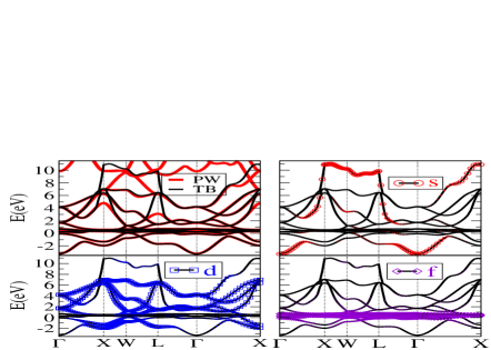
Figure 1: (Color online) Upper left panel shows the comparison between ab initio plane-wave based band structure (red thick lines) and the downfolded tight-binding result (black thin lines). Other three panels show projected weight of $6s$, $5d$ and $4f$-orbitals for each band.

In order to single out the many-body screening effects of the $5d$-channels, we first study the system with $\mathcal{H}_{2}$ treated at the Hartree-Fock mean-field level. The double counting term in Eq.17 represents the Hartree-Fock mean field interactions between the $4f$ and $5d$-electrons contained in $\mathcal{H}_{0}$, therefore, it exactly cancels the contribution from the $\mathcal{H}_{2}$ at the Hartree-Fock level and the whole electron Hamiltonian of the system reduces to the usual form with many-body Coulomb interactions only between the $4f$-electrons (i.e., $\mathcal{H}_{1}$). Proceeding with the Gutzwiller solution of $\mathcal{H}_{1}$, we include in our calculations $4f$-shell occupations of $f^{0}$, $f^{1}$ and $f^{2}$, resulting in 106 local $f$-configurations. Fig.2 shows the variation of orbital renormalization factors and orbital occupations with increasing Coulomb repulsion parameter $U_{ff}$. Due to cubic symmetry of $\gamma$-Ce, the $4f$-orbitals split into three groups with degeneracy of 3, 3, and 1. It can be seen that all the $z$-factors initially decrease with increasing $U_{ff}$.̇ A transition occurs near $U_{ff}^{T}=6eV$, beyond which the $z$-factors of the two sets of 3-fold degenerate $4f$-orbitals increase sharply while the $z$-factor of the singly degenerate $4f$-orbital decreases rapidly. Meanwhile, the orbital occupations exhibit similar variations near $U_{ff}^{T}=6eV$. The occupations of the triply degenerate orbital groups vanish swiftly as $U_{ff}$ exceeds $6eV$, while the singly degenerate orbital quickly approaches half-filling. These results support the physical picture of orbital-selective Mott transitionAnisimov02 ; Koga04 in which the $f$-electron in the system is redistributed among the $4f$-orbitals such that the singly degenerate $4f$-orbital approaches Mott localization with a half-filled band, while the remaining $4f$-orbitals become empty due to strong $f$-electron correlation effect. However, it has also been shown that a finite hybridization between the narrow correlated $f$-bands and the wide conduction bands (mainly 5d bands in this system) can suppress the Mott transition by Kondo screeningKotliar05 . The screened $U_{ff}^{scr}$ for $\gamma$-Ce has been calculated using constrained-LDA method and yields a value of $6eV$ which interestingly coincides with $U_{ff}^{T}$Macmahan98 . Therefore we choose the transition point in the $z$-$U$ curve as a fingerprint to identify the correct input $U_{ff}$ parameter for $\gamma$-Ce in the following calculations of different levels. We should emphasize that LDA itself can not capture the many-body Kondo screening effect. The constrained-LDA method gives reasonable estimation of the screened $U_{ff}^{scr}$ due to other processes, e.g., dielectric screening.

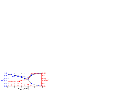
Figure 2: (Color online) Orbital renormalization factors $z_{\gamma}$ (left axis, blue solid symbols) and orbital occupations $n_{\gamma}^{0}$ (right axis, red open symbols) as functions of Coulomb repulsion parameter between $4f$-electrons $U_{ff}$. Square and circle are for the first two groups of $4f$-orbitals with degeneracy of 3. The third singly degenerate group is symbolized by up triangle. For paramagnetic solution we have $z_{\gamma}=z_{\gamma\uparrow}=z_{\gamma\downarrow}$ and $n_{\gamma}^{0}=n_{\gamma\uparrow}^{0}=n_{\gamma\downarrow}^{0}$.

We now study the effect of the many-body screening when the $5d$-electron screening is explicitly included by treating the $\mathcal{H}_{2}$ and $\mathcal{H}_{1}$ on equal footings with Gutzwiller variational wave functions constructed on the Gutzwiller local subspace consisting of both $4f$ and $5d$-orbitals. Any deviation of the calculation results from the mean field calculation described above will reflect the effect of many-body correlation effects arising from including $5d$-electrons in the Gutzwiller projector. Since we do not expect any significant correlation effect for $5d$-orbitals, we include all the local $5d$-configurations into account, which pushes the dimension of the local subspace to 108544. By taking advantage of sparse matrix techniques, a typical self-consistent calculation can still be done quite fast on a single processor. A set of Coulomb parameter $U_{fd}$ values of {1eV, 3eV, 5eV} are chosen with the successive inclusion of different number of many-body screening $5d$-channels to investigate the details of the many-body screening process. Our calculation results are shown in Fig.3 for the orbital renormalization factors $z_{\gamma}$ and in Fig.4 for the orbital occupations $n_{\gamma}^{0}$. One can see that the curves shift towards larger values of $U_{ff}$ in a nonlinear fashion with increasing Coulomb parameter $U_{fd}$ and increasing number of many-body $5d$-screening channels, indicating that the many-body screening is not a linear process. The correct input $U_{ff}$ parameter for $\gamma$-Ce in the calculations which corresponds to the transition point of the $z$-$U$ curve is pushed much closer to the bare Coulomb repulsion energy between $4f$-electrons ($\sim$23eV based on the neutral atomic $4f$-orbitals) with $U_{fd}\approx 5eV$ and all the $5d$-channels participating in many-body screening process. It should be pointed out that we encounter some numerical problem in searching solutions of the system on the smaller $U_{ff}$ side, however, this numerical difficulty will not affect our conclusion.

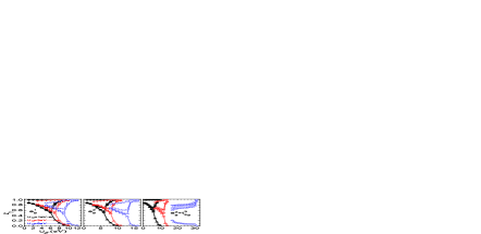
Figure 3: (Color online) The dependence of the orbital renormalization factor $z_{\gamma}$ on the Coulomb repulsion parameter between the $4f$-electrons $U_{ff}$, that between the $4f$ and $5d$-electrons $U_{fd}$, and the number of many-body screening $5d$-channels explicitly included in the Hamiltonian, which is 1 for the left panel (one of the $e_{g}$-orbitals), 2 for the middle (two $e_{g}$-orbitals), and 5 for the right (two $e_{g}$-orbitals and three $t_{2g}$-orbitals). The set of values of $U_{fd}$ scanned in the calculation are 1eV indicated by black solid symbols with solid lines, 3eV by red half-filled symbols with short-dashes, and 5eV by blue open symbols with short dots. The three distinct $z$-factors of $4f$-orbitals are depicted by the same symbols as in Fig.2 with the average $z$-factor for the participating d-channels by down triangles.

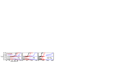
Figure 4: (Color online) The dependence of the orbital occupation $n_{\gamma}^{0}$ on the Coulomb repulsion parameter between the $4f$-electrons $U_{ff}$, that between the $4f$ and $5d$-electrons $U_{fd}$, and the number of many-body screening $5d$-channels explicitly included in the Hamiltonian. Plot settings are same as Fig.3.

To shed some light on the many-body screening mechanism, it is instructive to examine the variations of the local electronic configuration occupation probabilities $\left\{p_{\mathcal{F}}\right\}$, which are the new variational degrees of freedom in the Gutzwiller treatment. However, a straightforward analysis of the local electronic configurations can be rather tedious since its dimension is usually very large. In Fig.5 we present the sum of the occupation probabilities of the grouped local configurations according to the number of $f$-electrons occupied, which is closely related to the $z$-factors for the $4f$-orbitals. The local configurations with two $f$-electrons occupied can survive to larger $U_{ff}$ and the local configurations with one $f$-electron occupied will approach a full occupation at higher $U_{ff}$ by increasing $U_{fd}$. This tendency is consistent with the behavior of the $z$-factors for the $4f$-electrons. Another way to look at the many-body screening mechanism is to investigate the response of the screening $5d$-electrons when the many-body screening is turned on. Fig.3 shows that the $z$-factors for $5d$-orbitals are smaller than one, but are still quite large ($\gtrsim 0.8$). It implies that the $5d$-electrons rearrange themselves in the local subspace in a way deviating from Hartree-Fock mean field solution in order to effectively screen the interactions between the $4f$-electrons.

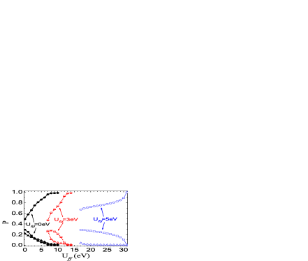
Figure 5: (Color online) The sum of occupation probabilities of some group of local electronic configurations as a function of $U_{ff}$ and $U_{fd}$ with all the $5d$ and $4f$-orbitals in the Gutzwiller local subspace. Squares are for the configurations with no $f$-electron occupied, circles for those with one $f$-electron, and up triangles for those with two $f$-electrons. $U_{fd}$=0eV is indicated by black solid symbols with solid lines, 3eV by red half-filled symbols with short-dashes, and 5eV by blue open symbols with short dots. The results with $U_{fd}$=0 are same as those with only $4f$ orbitals included in the Gutzwiller local subspace since there are no Coulomb interactions between $5d$ and $4f$-electrons.

By including Ce $5d$ and $4f$-orbitals into the Gutzwiller local subspace for the construction of Gutzwiller wave function., i.e., having $5d$-electrons treated in the same Gutzwiller level as $4f$-electrons beyond static Hartree-Fock mean-field approximation, we observe that the equivalent $U_{ff}$ is pushed towards its bare atomic value in $\gamma$-Ce. Therefore local many body response in the $5d$-channels is the dominant contribution in the screening process for $4f$-electrons in bulk Ce. This justifies our method in using single-site Gutzwiller treatment in this system. In some cases where significant screening effect comes from the atomic environmentBrink95 , we expect the generalized cluster-Gutzwiller treatment in parallel with cluster-DMFT would be usefulMaier05 .

IV Conclusion

A method for explicitly including many-body screening process into self-consistent calculations based on Gutzwiller variational wave function and Gutzwiller approximation has been proposed and applied to the tight-binding electronic structure calculation of $\gamma$-Ce. The resultant Coulomb repulsion parameter between $4f$-electrons $U_{ff}$ can be much larger than the corresponding screened $U_{ff}$ with moderate value of Coulomb repulsion parameter between $4f$ and $5d$-electrons $U_{fd}$. Assuming the dominant many-body screening effect for the strongly correlated orbitals (e.g., $4f$-orbitals for Ce) can be explicitly taken into account in this local approach, it is therefore of great interest to examine how the current scheme performs in full DFT-based self-consistent calculations where all the Coulomb repulsion energies between various orbitals in the Gutzwiller local subspace are directly obtained from atomic orbital integrations. Since the atomic orbitals are generally non-orthogonal, it is also highly worthwhile to extend the scheme from orthogonal orbitals to non-orthogonal orbitals. The proposed scheme here furnishes a promising way towards the realization of a self-consistent ab initio GDFT.

- (1) P. Hohenberg and W. Kohn, Phys. Rev. 136, B864 (1964).
- (2) W. Kohn and L. J. Sham, Phys. Rev. 140, A1133 (1965).
- (3) V. I. Anisimov, J. Zaanen, and O. K. Andersen, Phys. Rev. B 44, 943 (1991).
- (4) V. I. Anisimov, F. Aryasetiawan, and A. Lichtenstein, Journal of Physics-Condensed Matter 9, 767 (1997).
- (5) V. I. Anisimov, A. Poteryaev, M. Korotin, A. Anokhin, and G. Kotliar, Journal of Physics-Condensed Matter 9, 7359 (1997)
- (6) G. Kotliar, S. Y. Savrasov, K. Haule, V. S. Oudovenko, O. Parcollet, and C. A. Marianetti, Rev. Mod. Phys. 78, 865 (2006).
- (7) X. Y. Deng, X. Dai, and Z. Fang, Europhysics Letters 83, 37008 (2008).
- (8) X. Y. Deng, L. Wang, X. Dai, and Z. Fang, Phys. Rev. B 79, 075114-20 (2009).
- (9) O. Gunnarsson, O. K. Andersen, O. Jepsen, and J. Zaanen, Phys. Rev. B 39, 1708 (1989).
- (10) M. Springer and F. Aryasetiawan, Phys. Rev. B 57, 4364 (1998).
- (11) T. Kotani, Journal of Physics-Condensed Matter 12, 2413 (2000).
- (12) F. Aryasetiawan, M. Imada, A. Georges, G. Kotliar, S. Biermann, and A. I. Lichtenstein, Phys. Rev. B 70, 195104 (2004).
- (13) K. M. Ho, J. Schmalian, and C. Z. Wang, Phys. Rev. B 77, 073101 (2008).
- (14) M. C. Gutzwiller, Phys. Rev. Lett. 10, 159 (1963).
- (15) M. C. Gutzwiller, Phys. Rev. 137, A1726 (1965).
- (16) J. Bünemann and F. Gebhard, Phys. Rev. B 76, 193104-4 (2007).
- (17) L. M. Falicov and J. C. Kimball, Phys. Rev. Lett. 22, 997 (1969).
- (18) V. I. Anisimov, I. V. Solovyev, M. A. Korotin, M. T. Czyzdotyk, and G. A. Sawatzky, Phys. Rev. B 48, 16929 (1993).
- (19) M. T. Czyżyk and G. A. Sawatzky, Phys. Rev. B 49, 14211 (1994).
- (20) J. Bünemann, F. Gebhard, and R. Thul, Phys. Rev. B 67, 075103 (2003).
- (21) Y. X. Yao, Ph.D. Thesis, Iowa State University, USA, 2009.
- (22) W. C. Lu, C. Z. Wang, T. L. Chan, K. Ruedenberg, and K. M. Ho, Phys. Rev. B 70, 041101 (2004).
- (23) T. L. Chan, Y. X. Yao, C. Z. Wang, W. C. Lu, J. Li, X. F. Qian, S. Yip, and K. M. Ho, Physical Review B 76, 205119 (2007).
- (24) X. F. Qian, J. Li, L. Qi, C. Z. Wang, T. L. Chan, Y. X. Yao, K. M. Ho, and S. Yip, Physical Review B 78, 245112 (2008).
- (25) Y. X. Yao, C. Z. Wang, G. P. Zhang, M. Ji, and K. M. Ho, Journal of Physics-Condensed Matter 21, 235501 (2009).
- (26) Vienna ab initio Simulation Package. G. Kresse and J. Hafner, Phys. Rev. B 47, 558 (1993); G. Kresse and J. Furthmuller, ibid 54, 11169 (1996).
- (27) V. I. Anisimov, I. A. Nekrasov, D. E. Kondakov, T. M. Rice, and M. Sigrist, The European Physical Journal B - Condensed Matter and Complex Systems 25, 191-201 (2002).
- (28) A. Koga, N. Kawakami, T. M. Rice, and M. Sigrist, Phys. Rev. Lett. 92, 216402 (2004).
- (29) L. de’ Medici, A. Georges, G. Kotliar, and S. Biermann, Phys. Rev. Lett. 95, 066402 (2005).
- (30) A. K. McMahan, C. Huscroft, R. T. Scalettar, and E. L. Pollock, Journal Of Computer-Aided Materials Design 5, 131-162 (1998).
- (31) J. van den Brink, M. B. J. Meinders, J. Lorenzana, R. Eder, and G. A. Sawatzky, Phys. Rev. Lett. 75, 4658 (1995).
- (32) T. Maier, M. Jarrell, T. Pruschke, and M. H. Hettler, Rev. Mod. Phys. 77, 1027 (2005).