A Non-Iterative Solution to the Four-Point Three-Views Pose Problem in Case of Collinear Cameras

Abstract.

We give a non-iterative solution to a particular case of the four-point three-views pose problem when three camera centers are collinear. Using the well-known Cayley representation of orthogonal matrices, we derive from the epipolar constraints a system of three polynomial equations in three variables. The eliminant of that system is a multiple of a 36th degree univariate polynomial. The true (unique) solution to the problem can be expressed in terms of one of real roots of that polynomial. Experiments on synthetic data confirm that our method is robust enough even in case of planar configurations.

1. Introduction

We first recall some definitions from multiview geometry and formulate the problem in question, see [3, 8] for details. A pinhole camera is a triple $(O,\Pi,p)$, where $\Pi$ is an image plane, $p$ is a central projection of points in 3-dimensional Euclidean space onto $\Pi$, and $O$ is a camera center (center of the projection $p$). The focal length is the distance between $O$ and $\Pi$, the orthogonal projection of $O$ onto $\Pi$ is called the principal point. A pinhole camera is called calibrated if all its intrinsic parameters (such as focal length and principal point’s coordinates) are known.

Problem 1 (The four-point three-views pose problem).

Let us consider three calibrated pinhole cameras with centers $O_{1}$, $O_{2}$, $O_{3}$ and four scene points $P_{1}$, …, $P_{4}$ being in front of the cameras in 3-dimensional Euclidean space, see Figure 1. In every local coordinate system $O_{j}xyz$, associated with the $j$th camera, the homogeneous coordinates $\begin{pmatrix}x_{ji}&y_{ji}&1\end{pmatrix}^{\mathrm{T}}$ of all $P_{i}$’s are only known. One must find the relative position and orientation of the second and third cameras with respect to the first one and the coordinates of all $P_{i}$’s in $O_{1}xyz$.

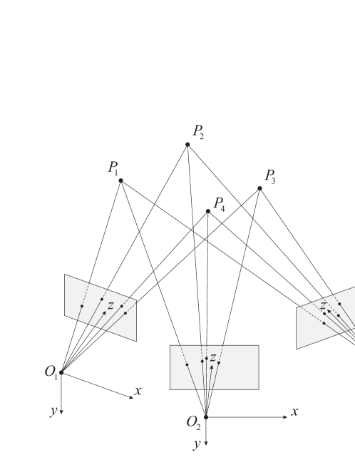
Figure 1. To formulation of the four-point three-views pose problem

Remark 1.

It is well-known that the solution to Problem 1 is only defined up to an overall scale. That is, multiplying the coordinates of all the reconstructed points by any $\lambda>0$, we get another solution to Problem 1. In order to resolve this ambiguity, we assume from now on that the length of the baseline joining $O_{1}$ and $O_{2}$ is given and equals $d$.

Problem 1 is known to be slightly over-determined and in general to have a unique solution [4, 10]. The only iterative approach to the problem has been proposed in [9].

In the paper presented, we consider a light (but still highly nontrivial) version of Problem 1 when the three camera centers $O_{1}$, $O_{2}$ and $O_{3}$ are collinear. We use the method of paper [7] to derive a relatively simple system of three polynomials in three variables. It is shown that the eliminant of that system is a multiple of a 36th degree irreducible univariate polynomial. It is conjectured that in general one of its real roots encodes a solution to Problem 1. Experiments show that our approach is comparable in accuracy with the existing five-point solvers.

Here we outline our algorithm:

1. Transform the initial data $x_{ji}$, $y_{ji}$ in such a way that $x_{j1}=y_{j1}=x_{j2}=0$, $j=1,2,3$, applying rotations (1).

2. Derive from the epipolar constraints six polynomials $f^{(j)}_{i}$ by (12) and one polynomial $f^{\text{mix}}$ by (13).

3. Construct system (29) of three polynomials in three variables.

4. Using resultants and polynomial divisions, derive a 36th degree univariate polynomial $\mathcal{S}$.

5. For every real root of $\mathcal{S}$, find the matrices $R^{(2)}$, $R^{(3)}$ and $[t]_{\times}$ by (7) and (10) respectively.

6. Find the coordinates of $O_{2}$, $O_{3}$ and $P_{i}$ by (34), (35) and (36) respectively.

The paper is organized as follows. In Section 2, we describe in detail our algorithm. In Section 3, we make a comparison of our algorithm with the five-point Li-Hartley solver [6] on two sets of synthetic data. In Section 4, we discuss the results of the paper.

2. Description of the algorithm

2.1. Transformation of the initial data

Initial data for our algorithm are the values $x_{ji}$, $y_{ji}$ for $j=1,2,3,$ and $i=1,\ldots,4$, as well as the distance $d$ (see Remark 1).

Without loss of generality, we can set $x_{j1}=y_{j1}=x_{j2}=0$ for $j=1,2,3$. If $x_{j1}$, $y_{j1}$ and $x_{j2}$ differ from zero, we rotate $O_{j}xyz$ to $O_{j}\tilde{x}\tilde{y}\tilde{z}$ with the matrix

$$\rho_{j}=R_{\varphi_{j}}R_{\theta_{j}}R_{\psi_{j}},$$ (1)

where $R_{\varphi_{j}}$, $R_{\theta_{j}}$, $R_{\psi_{j}}$ are rotations through the angles $\varphi_{j}$, $\theta_{j}$, $\psi_{j}$ respectively around the axes $O_{j}z$, $O_{j}y$, $O_{j}x$ respectively. The angles can be expressed by the formulas:

$$\begin{split}\tan\psi_{j}&=y_{j1},\\ \tan\theta_{j}&=\frac{x_{j1}}{\sqrt{1+y_{j1}^{2}}},\\ \tan\varphi_{j}&=\frac{x_{j2}(1+y_{j1}^{2})-x_{j1}(1+y_{j1}y_{j2})}{(y_{j2}-y_{j1})\sqrt{1+x_{j1}^{2}+y_{j1}^{2}}}.\end{split}$$ (2)

One then verifies that $\tilde{x}_{j1}=\tilde{y}_{j1}=\tilde{x}_{j2}=0$. Besides, the depth of $P_{1}$ from the camera center $O_{j}$ is

$$\sqrt{1+x_{j1}^{2}+y_{j1}^{2}}>0,$$

i.e. the point $P_{1}$ remains to be in front of all the cameras.

We will see that the above transformation of the initial data, being quite simple, noticeably simplify our further computations.

2.2. Epipolar constraints and essential matrices

From now on we assume that the three camera centers $O_{1}$, $O_{2}$ and $O_{3}$ are collinear.

Denote by $\begin{pmatrix}x^{\prime}_{ji}&y^{\prime}_{ji}&1\end{pmatrix}^{\mathrm{T}}$ and $\mathbf{t}=\begin{pmatrix}t_{x}&t_{y}&t_{z}\end{pmatrix}^{\mathrm{T}}$ the directing vectors of $O_{j}P_{i}$ and $O_{1}O_{2}$ respectively in the world coordinate system $O_{1}xyz$. It follows that the directing vector of $O_{1}O_{3}$ is $\sigma\mathbf{t}$, where $\sigma$ is either $+1$ or $-1$.

Let Cartesian coordinates of $P_{i}$ and $O_{j}$ be $(x_{P_{i}},y_{P_{i}},z_{P_{i}})$ and $(x_{O_{j}},y_{O_{j}},z_{O_{j}})$ respectively. Then, it is easy to see that ($j=2,3$; $i=1,\ldots,4$)

$$\begin{split}(x_{1i}-x^{\prime}_{ji})\,t_{z}z_{P_{i}}&=(t_{x}-t_{z}x^{\prime}_{ji})\,z_{O_{j}},\\ (y_{1i}-y^{\prime}_{ji})\,t_{z}z_{P_{i}}&=(t_{y}-t_{z}y^{\prime}_{ji})\,z_{O_{j}}.\end{split}$$ (3)

Eliminating $z_{P_{i}}$, $z_{O_{2}}$ and $z_{O_{3}}$ from this system, we get

$$\begin{split}t_{x}(y^{\prime}_{2i}-y_{1i})+t_{y}(x_{1i}-x^{\prime}_{2i})+t_{z}(y_{1i}x^{\prime}_{2i}-x_{1i}y^{\prime}_{2i})&=0,\\ t_{x}(y^{\prime}_{3i}-y_{1i})+t_{y}(x_{1i}-x^{\prime}_{3i})+t_{z}(y_{1i}x^{\prime}_{3i}-x_{1i}y^{\prime}_{3i})&=0.\end{split}$$ (4)

Consider matrices $R^{(j)}\in\mathrm{SO}(3)$, $j=2,3$, rotating $O_{j}xyz$ so that

$$\omega_{ji}\begin{pmatrix}x^{\prime}_{ji}\\ y^{\prime}_{ji}\\ 1\end{pmatrix}=R^{(j)}\begin{pmatrix}x_{ji}\\ y_{ji}\\ 1\end{pmatrix}.$$ (5)

where $\omega_{ji}$ is called the depth of the point $P_{i}$ from the camera center $O_{j}$. Then, it is easy to see that (4) is equivalent to the so-called epipolar constraints:

$$\begin{pmatrix}x_{1i}&y_{1i}&1\end{pmatrix}E^{(j)}\begin{pmatrix}x_{2i}\\ y_{2i}\\ 1\end{pmatrix}=0,$$ (6)

where $E^{(j)}=[t]_{\times}R^{(j)}$ is called the essential matrix and $[t]_{\times}$ is the skew-symmetric cross-product operator.

2.3. Seven polynomials in six variables

Our approach is based on the following well-known result.

Theorem 1 ([1]).

If a matrix $R\in\mathrm{SO}(3)$ is not a rotation through the angle $\pi$ about certain axis, then $R$ can be represented as

$$\frac{1}{\Delta}\begin{pmatrix}1-u^{2}+w^{2}(1-v^{2})&2(vw^{2}-u)&2w(u+v)\\ 2(vw^{2}+u)&1-u^{2}-w^{2}(1-v^{2})&2w(uv-1)\\ 2w(u-v)&2w(uv+1)&1+u^{2}-w^{2}(1+v^{2})\end{pmatrix},$$ (7)

where $\Delta=1+u^{2}+w^{2}(1+v^{2})$.

Let $Oxyz$ and $OXYZ$ be two coordinate systems with a common origin and of the same handedness. Then the Euler angles, transforming $Oxyz$ to $OXYZ$, are defined as [5]:

• $\varphi$ is the angle between the $x$-axis and the line of nodes, i.e. the line of intersection of the $xy$ and the $XY$ coordinate planes.

• $\theta$ is the angle between the $z$-axis and the $Z$-axis.

• $\psi$ is the angle between the line of nodes and the $X$-axis.

Remark 2.

By direct calculation one verifies that the Euler angles $\varphi$, $\theta$ and $\psi$ can be expressed in terms of the parameters $u$, $v$ and $w$ as follows:

$$\begin{split}\varphi&=\arctan\frac{u+v}{1-uv},\\ \psi&=\arctan\frac{u-v}{1+uv},\\ \theta&=\pm 2\arctan w\sqrt{\frac{1+v^{2}}{1+u^{2}}}.\end{split}$$ (8)

Lemma 1.

Let $\varphi_{j}$, $\theta_{j}$ and $\psi_{j}$ be Euler angles parameterizing the matrix $R^{(j)}$. In case of collinear camera centers $O_{1}$, $O_{2}$ and $O_{3}$, the following identity holds:

$$\tan\varphi_{2}=\tan\varphi_{3}.$$

Proof.

Due to the condition $x_{j1}=y_{j1}=0$, $j=1,2,3$, the $z$-axes of all $O_{j}xyz$ intersect in the only point $P_{1}$. Since $O_{1}$, $O_{2}$ and $O_{3}$ are collinear, the lines of nodes of $O_{2}xyz$ and $O_{3}xyz$ are identical and hence, by definition, $\varphi_{2}=\varphi_{3}\mod\pi$. ∎

Lemma 2.

Let $E^{(j)}(u,v,w)$ be an essential matrix subject to system (6). If

$$\begin{split}u^{\prime}_{j}&=-u_{j}^{-1},\\ v^{\prime}_{j}&=-v_{j}^{-1},\\ w^{\prime}_{j}&=-\frac{v_{j}}{u_{j}}\,\frac{y_{12}w_{j}(v_{j}+u_{j})+y_{j2}w_{j}(v_{j}-u_{j})-2y_{12}y_{j2}u_{j}}{y_{12}(v_{j}+u_{j})-y_{j2}(v_{j}-u_{j})+2y_{12}y_{j2}v_{j}w_{j}},\end{split}$$ (9)

then $E^{(j)}(u^{\prime}_{j},v^{\prime}_{j},w^{\prime}_{j})=-E^{(j)}(u_{j},v_{j},w_{j})$.

Proof.

Let $E^{(j)}=[t]_{\times}R^{(j)}$ be subject to (6). Then, from the first two equations of (6) (for $i=1,2$) we find

$$\begin{split}t_{x}&=t_{z}\,\frac{R^{(j)}_{13}(R^{(j)}_{12}y_{j2}+R^{(j)}_{13})y_{12}}{(R^{(j)}_{23}R^{(j)}_{12}-R^{(j)}_{13}R^{(j)}_{22})y_{j2}+R^{(j)}_{13}(R^{(j)}_{32}y_{j2}+R^{(j)}_{33})y_{12}},\\ t_{y}&=t_{x}\,\frac{R^{(j)}_{23}}{R^{(j)}_{13}}=t_{x}\,\frac{u_{j}v_{j}-1}{u_{j}+v_{j}},\end{split}$$ (10)

where $R^{(j)}_{ik}$ is the $(i,k)$th entry of $R^{(j)}$. Substituting these values into the matrix $[t]_{\times}$, we get $E^{(j)}=E^{(j)}(u_{j},v_{j},w_{j})$. By a straightforward computation, we find that the equation $E^{(j)}(u_{j},v_{j},w_{j})+E^{(j)}(u^{\prime}_{j},v^{\prime}_{j},w^{\prime}_{j})=0$ has the only solution (9). ∎

Since system (4) is linear and homogeneous in $t_{x}$, $t_{y}$ and $t_{z}$, it has a nontrivial solution if and only if $\operatorname{rank}\begin{pmatrix}Q^{(2)}\\ Q^{(3)}\end{pmatrix}\leq 2$, where

$$Q^{(j)}=\begin{pmatrix}y^{\prime}_{j1}&-x^{\prime}_{j1}&0\\ y^{\prime}_{j2}-y_{12}&-x^{\prime}_{j2}&y_{12}x^{\prime}_{j2}\\ y^{\prime}_{j3}-y_{13}&x_{13}-x^{\prime}_{j3}&y_{13}x^{\prime}_{j3}-x_{13}y^{\prime}_{j3}\\ y^{\prime}_{j4}-y_{14}&x_{14}-x^{\prime}_{j4}&y_{14}x^{\prime}_{j4}-x_{14}y^{\prime}_{j4}\end{pmatrix}.$$ (11)

Let $i=i_{(\alpha,\beta,\gamma)}$ number triples from $\{1,2,3,4\}$ so that $i_{(1,2,3)}=1$, $i_{(1,2,4)}=2$, $i_{(1,3,4)}=3$. Then, it follows that $\det Q^{(j)}_{i}=0$, where $Q^{(j)}_{i}$ is a $3\times 3$ submatrix of $Q^{(j)}$ corresponding to the rows $\alpha$, $\beta$ and $\gamma$. Thus, we get a system

$$f^{(j)}_{i}=\det Q^{(j)}_{i}\,\frac{\Delta_{j}^{2}\,\omega_{j\alpha}\omega_{j\beta}\omega_{j\gamma}}{w_{j}}=0,\quad j=2,3,\quad i=1,2,3.$$ (12)

where $\Delta_{j}=1+u_{j}^{2}+w_{j}^{2}(1+v_{j}^{2})$ and, for instance, $\omega_{j\alpha}$ is the depth of the point $P_{\alpha}$ from $O_{j}$ (cf. (5)). One verifies that in general each $f^{(j)}_{i}$ is an irreducible polynomial in $u_{j}$, $v_{j}$, $w_{j}$ of the sixth total degree.

Remark 3.

In (12), we assume that $w_{j}\neq 0$. No solution is lost here, since $w_{j}=0$ means that the matrix $R^{(j)}$ is a rotation about the $z$-axis, which may only occur if $O_{j}=O_{1}$.

In addition to (12), we can also obtain more polynomial equations by treating the rows of both $Q^{(2)}$ and $Q^{(3)}$. For example, consider a submatrix $Q^{\text{mix}}$ of $\begin{pmatrix}Q^{(2)}\\ Q^{(3)}\end{pmatrix}$ consisting of the first two rows of $Q^{(2)}$ and the second row of $Q^{(3)}$. Then,

$$f^{\text{mix}}=\det Q^{\text{mix}}\,\frac{\Delta_{2}^{2}\Delta_{3}\,\omega_{21}\omega_{22}\omega_{32}}{x^{\prime}_{21}}=0,$$ (13)

where we assume that $x^{\prime}_{21}\neq 0$. In general, $f^{\text{mix}}$ is an irreducible polynomial in $u_{2}$, $v_{2}$, $w_{2}$, $u_{3}$, $v_{3}$, $w_{3}$ of the seventh total degree.

2.4. Two polynomials in three variables

In this subsection, we deal with the polynomials $f^{(j)}_{i}$ defined in (12). We are going to eliminate the variables $w_{2}$ and $w_{3}$ from them and then simplify the obtained polynomials using the transformations (9).

Notice that every polynomial $f^{(j)}_{i}$ is of the second degree in $w_{j}$, i.e.

$$f^{(j)}_{i}=a^{(j)}_{i}w_{j}^{2}+b^{(j)}_{i}w_{j}+c^{(j)}_{i},$$ (14)

where $a^{(j)}_{i}$, $b^{(j)}_{i}$, $c^{(j)}_{i}$ are polynomials in $u_{j}$ and $v_{j}$. Consider a matrix

$$F^{(j)}=\begin{pmatrix}a^{(j)}_{1}&b^{(j)}_{1}&c^{(j)}_{1}\\ a^{(j)}_{2}&b^{(j)}_{2}&c^{(j)}_{2}\\ a^{(j)}_{3}&b^{(j)}_{3}&c^{(j)}_{3}\end{pmatrix}.$$

Then, system (12) (for each $j$) has a solution if and only if $\det F^{(j)}=0$, i.e. we get two polynomial equations:

$$g^{(j)}(u_{j},v_{j})=\det F^{(j)}=0,\quad j=2,3.$$ (15)

The polynomials $g^{(2)}$ and $g^{(3)}$ are of the 10th total degree in the variables $u_{2}$, $v_{2}$ and $u_{3}$, $v_{3}$ respectively. We can reduce the total number of variables to three by introducing a new variable

$$s=\frac{u_{2}+v_{2}}{1-u_{2}v_{2}}=\frac{u_{3}+v_{3}}{1-u_{3}v_{3}},$$

where the second equality holds due to Lemma 1. Note that the variable $s$ is unchanged under the transformations (9), i.e.

$$s^{\prime}=\frac{u^{\prime}_{j}+v^{\prime}_{j}}{1-u^{\prime}_{j}v^{\prime}_{j}}=\frac{u_{j}+v_{j}}{1-u_{j}v_{j}}=s.$$

Substituting

$$v_{j}=\frac{s-u_{j}}{1+su_{j}}.$$ (16)

to (15), we get

$$h^{(j)}(u_{j},s)=(1+su_{j})^{6}\,g^{(j)}(u_{j},\frac{s-u_{j}}{1+su_{j}}).$$

By Lemma 2, $h^{(j)}(u^{\prime}_{j},s^{\prime})=h^{(j)}(-u_{j}^{-1},s)=0$. Moreover, $h^{(j)}$ has a special symmetric form:

$$h^{(j)}=u_{j}^{12}\sum\limits_{k=0}^{12}p^{(j)}_{k}\left[u_{j}^{12-k}+(-u_{j})^{k-12}\right],$$ (17)

where $p^{(j)}_{k}$ are 6th degree polynomials in $s$. Due to the above symmetry, we can introduce a new variable $\tilde{u_{j}}=u_{j}-u_{j}^{-1}$, and then transform $h_{j}$ to the polynomial

$$\tilde{h}^{(j)}=\sum\limits_{k=0}^{6}\tilde{p}^{(j)}_{k}\tilde{u}_{j}^{k},$$ (18)

where

$$\begin{split}\tilde{p}^{(j)}_{2k}&=\sum\limits_{i=k}^{6}p^{(j)}_{12-2i}\varkappa_{i,k},\\ \tilde{p}^{(j)}_{2k+1}&=\sum\limits_{i=k}^{5}p^{(j)}_{11-2i}\varkappa_{i+1/2,k+1/2},\end{split}$$ (19)

and $\varkappa_{i,k}$ denotes the sum of two binomial coefficients:

$$\varkappa_{i,k}=\binom{i+k}{i-k}+\binom{i+k-1}{i-k-1}.$$ (20)

As a result, we have two irreducible polynomials $\tilde{h}^{(2)}(\tilde{u}_{2},s)$ and $\tilde{h}^{(3)}(\tilde{u}_{3},s)$ of the 12th total degree each. In order to solve the problem, we need at least one more polynomial in the variables $\tilde{u}_{2}$, $\tilde{u}_{3}$ and $s$.

2.5. One more polynomial in three variables

Let us consider the polynomial $f^{\text{mix}}$ defined in (13). As in the previous subsection, we are going to eliminate the variables $w_{2}$ and $w_{3}$ from $f^{\text{mix}}$ and then simplify the result using transformations (9).

First, we notice that $f^{\text{mix}}$ is of the second degree in the variable $w_{2}$:

$$f^{\text{mix}}=a^{\text{mix}}w_{2}^{2}+b^{\text{mix}}w_{2}+c^{\text{mix}},$$ (21)

where $a^{\text{mix}}$, $b^{\text{mix}}$, $c^{\text{mix}}$ are polynomials in the remaining five variables. Consider a matrix

$$F^{\text{mix}}=\begin{pmatrix}a^{(2)}_{1}&b^{(2)}_{1}&c^{(2)}_{1}\\ a^{(2)}_{2}&b^{(2)}_{2}&c^{(2)}_{2}\\ a^{\text{mix}}&b^{\text{mix}}&c^{\text{mix}}\end{pmatrix}.$$

The three polynomials $f^{(2)}_{1}$, $f^{(2)}_{2}$ and $f^{\text{mix}}$ have a common solution if and only if $\det F^{\text{mix}}=0$. This yields

$$\hat{f}^{\text{mix}}=\frac{\det F^{\text{mix}}}{(y_{12}^{2}-y_{22}^{2})u_{2}^{2}+2(y_{12}^{2}+2y_{12}^{2}y_{22}^{2}+y_{22}^{2})u_{2}v_{2}+(y_{12}^{2}-y_{22}^{2})v_{2}^{2}}=0.$$ (22)

One verifies that the polynomial $\hat{f}^{\text{mix}}$ is in turn of the second degree in $w_{3}$, i.e.

$$\hat{f}^{\text{mix}}=\hat{a}^{\text{mix}}w_{3}^{2}+\hat{b}^{\text{mix}}w_{3}+\hat{c}^{\text{mix}},$$ (23)

where $\hat{a}^{\text{mix}}$, $\hat{b}^{\text{mix}}$, $\hat{c}^{\text{mix}}$ are polynomials in $u_{2}$, $v_{2}$, $u_{3}$ and $v_{3}$. Similarly, we define the matrix

$$\hat{F}^{\text{mix}}=\begin{pmatrix}a^{(3)}_{1}&b^{(3)}_{1}&c^{(3)}_{1}\\ a^{(3)}_{2}&b^{(3)}_{2}&c^{(3)}_{2}\\ \hat{a}^{\text{mix}}&\hat{b}^{\text{mix}}&\hat{c}^{\text{mix}}\end{pmatrix},$$

and from the constraint $\det\hat{F}^{\text{mix}}=0$ obtain the polynomial

$$g^{\text{mix}}=\frac{\det\hat{F}^{\text{mix}}}{(y_{12}^{2}-y_{32}^{2})u_{3}^{2}+2(y_{12}^{2}+2y_{12}^{2}y_{32}^{2}+y_{32}^{2})u_{3}v_{3}+(y_{12}^{2}-y_{32}^{2})v_{3}^{2}}=0.$$ (24)

Substituting (16) to $g^{\text{mix}}=g^{\text{mix}}(u_{2},v_{2},u_{3},v_{3})$, we get

$$h^{\text{mix}}(u_{2},u_{3},s)=\frac{(1+su_{2})^{3}(1+su_{3})^{3}\,g^{\text{mix}}(u_{2},\frac{s-u_{2}}{1+su_{2}},u_{3},\frac{s-u_{3}}{1+su_{3}})}{(1+u_{2}^{2})(1+u_{3}^{2})(x_{13}+y_{13}s)(x_{14}+y_{14}s)}.$$ (25)

Remark 4.

The denominators in (22), (24) and (25) are supposed to be nonzero. By a straightforward computation, one verifies that in general their roots do not give a solution to Problem 1.

The polynomial $h^{\text{mix}}$ has a special symmetric form:

$$h^{\text{mix}}=u_{2}^{4}u_{3}^{4}\sum\limits_{k=0}^{4}\sum\limits_{m=0}^{4}p^{\text{mix}}_{k,m}\,[u_{2}^{4-k}+(-u_{2})^{k-4}][u_{3}^{4-m}+(-u_{3})^{m-4}],$$ (26)

where $p^{\text{mix}}_{k,m}$ are polynomials in $s$. Substituting $\tilde{u_{j}}=u_{j}-u_{j}^{-1}$, we transform $h^{\text{mix}}$ to the polynomial

$$\tilde{h}^{\text{mix}}=\sum\limits_{k=0}^{2}\sum\limits_{m=0}^{2}\tilde{p}^{\text{mix}}_{k,m}\,\tilde{u}_{2}^{k}\,\tilde{u}_{3}^{m},$$ (27)

where

$$\begin{split}\tilde{p}^{\text{mix}}_{2k,2m}&=\sum\limits_{i=k}^{2}\sum\limits_{j=m}^{2}p^{\text{mix}}_{4-2i,4-2j}\varkappa_{i,k}\varkappa_{j,m},\\ \tilde{p}^{\text{mix}}_{2k,2m+1}&=\sum\limits_{i=k}^{2}\sum\limits_{j=m}^{1}p^{\text{mix}}_{4-2i,3-2j}\varkappa_{i,k}\varkappa_{j+1/2,m+1/2},\\ \tilde{p}^{\text{mix}}_{2k+1,2m}&=\sum\limits_{i=k}^{1}\sum\limits_{j=m}^{2}p^{\text{mix}}_{3-2i,4-2j}\varkappa_{i+1/2,k+1/2}\varkappa_{j,m},\\ \tilde{p}^{\text{mix}}_{2k+1,2m+1}&=\sum\limits_{i=k}^{1}\sum\limits_{j=m}^{1}p^{\text{mix}}_{3-2i,3-2j}\varkappa_{i+1/2,k+1/2}\varkappa_{j+1/2,m+1/2},\end{split}$$ (28)

and $\varkappa_{i,k}$ is given by (20).

2.6. Some notions from elimination theory

In this subsection, we briefly recall some notions from elimination theory, see [2] for details.

Given an ideal $J=\langle f_{1},\ldots,f_{m}\rangle\subset\mathbb{C}[x_{1},\ldots,x_{n}]$, the $l$th elimination ideal $J_{l}$ is defined by $J_{l}=J\cap\mathbb{C}[x_{l+1},\ldots,x_{n}]$, i.e. $J_{l}$ consists of all consequences of $f_{1}=\cdots=f_{m}=0$ eliminating the variables $x_{1}$, …, $x_{l}$. The generator of $J_{n-1}$ is called the eliminant of $J$ in the variable $x_{n}$.

As is well-known, the best way for finding elimination ideals is computing a Gröbner basis of $J$ with respect to the pure lexicographic ordering $x_{1}>\cdots>x_{n}$. However, in many cases this computation is practically impossible because of bounded computer resources. For these cases some roundabout ways, such as theory of resultants, should be applied.

Let $f_{1}=\sum\limits_{i=0}^{p}a_{i}x_{1}^{i}$ and $f_{2}=\sum\limits_{i=0}^{q}b_{i}x_{1}^{i}$, where $a_{i},b_{i}\in\mathbb{C}[x_{2},\ldots,x_{n}]$, be polynomials in $\mathbb{C}[x_{2},\ldots,x_{n}][x_{1}]$. The Sylvester matrix $\operatorname{Syl}_{x_{1}}(f_{1},f_{2})=(s_{kl})_{k,l=1}^{p+q}$ of $f_{1}$ and $f_{2}$ with respect to $x_{1}$ is defined by

$$\begin{split}s_{j,j+i}&=a_{p-i},\\ s_{p+q-j+1,j+i}&=b_{q-i},\end{split}$$

and all other entries of $\operatorname{Syl}_{x_{1}}(f_{1},f_{2})$ are equal to zero. The resultant of $f_{1}$ and $f_{2}$ with respect to $x_{1}$, denoted $\mathcal{R}_{x_{1}}(f_{1},f_{2})$, is the determinant of the Sylvester matrix, i.e. $\mathcal{R}_{x_{1}}(f_{1},f_{2})=\det\operatorname{Syl}_{x_{1}}(f_{1},f_{2})$. The following lemma states the relation between resultants and elimination ideals.

Lemma 3 ([2]).

Let $f_{1},f_{2}\in\mathbb{C}[x_{1},\ldots,x_{n}]$ have positive degree in $x_{1}$. Then, $\mathcal{R}_{x_{1}}(f_{1},f_{2})\in J_{1}$.

2.7. Thirty-sixth degree univariate polynomial

At this step, we have derived the following polynomial system in the variables $\tilde{u}_{2}$, $\tilde{u}_{3}$ and $s$:

$$\begin{split}\tilde{h}^{(2)}&=[4]s^{2}\tilde{u}_{2}^{6}+[5]s\tilde{u}_{2}^{5}+[6]\tilde{u}_{2}^{4}+[6]\tilde{u}_{2}^{3}+[6]\tilde{u}_{2}^{2}+[6]\tilde{u}_{2}+[6],\\ \tilde{h}^{(3)}&=[4]s^{2}\tilde{u}_{3}^{6}+[5]s\tilde{u}_{3}^{5}+[6]\tilde{u}_{3}^{4}+[6]\tilde{u}_{3}^{3}+[6]\tilde{u}_{3}^{2}+[6]\tilde{u}_{3}+[6],\\ \tilde{h}^{\text{mix}}&=[3]s\tilde{u}_{2}^{2}\tilde{u}_{3}^{2}+[4]\tilde{u}_{2}^{2}\tilde{u}_{3}+[4]\tilde{u}_{2}\tilde{u}_{3}^{2}+[4]\tilde{u}_{2}^{2}+[4]\tilde{u}_{2}\tilde{u}_{3}+[4]\tilde{u}_{3}^{2}+[4]\tilde{u}_{2}+[4]\tilde{u}_{3}+[4],\end{split}$$ (29)

where $[n]$ means an $n$th degree polynomial in the variable $s$.

Let us consider an ideal $J=\langle\tilde{h}^{(2)},\tilde{h}^{(3)},\tilde{h}^{\text{mix}}\rangle\subset\mathbb{C}[\tilde{u}_{2},\tilde{u}_{3},s]$ and denote its elimination ideals by $J_{1}=J\cap\mathbb{C}[\tilde{u}_{3},s]$ and $J_{2}=J\cap\mathbb{C}[s]$.

By direct computation, we find

$$\mathcal{R}_{\tilde{u}_{2}}(\tilde{h}^{(2)},\tilde{h}^{\text{mix}})=r(s^{2}+1)^{6}\,\mathcal{S}_{2}^{2}\in J_{1},$$ (30)

where $r$ is a 28th total degree polynomial in the variables $\tilde{u}_{3}$ and $s$, $\mathcal{S}_{2}$ and $\mathcal{S}_{3}$ (see below formula (32)) are 4th degree polynomials in the variable $s$ with the known (rather cumbersome) coefficients. For example, the trailing coefficient of $\mathcal{S}_{k}$ is

$$y_{k2}^{2}\left[x_{14}x_{k3}(y_{12}-y_{13})(y_{k2}-y_{k4})-x_{13}x_{k4}(y_{12}-y_{14})(y_{k2}-y_{k3})\right]\\ \times\left[x_{13}(y_{12}-y_{14})(x_{k4}^{2}-x_{k3}x_{k4}-y_{k3}y_{k4}+y_{k4}^{2})\right.\\ \left.+x_{14}(y_{12}-y_{13})(x_{k3}^{2}-x_{k3}x_{k4}-y_{k3}y_{k4}+y_{k3}^{2})\right].$$ (31)

Further,

$$\mathcal{R}_{\tilde{u}_{3}}(\tilde{h}^{(3)},\mathcal{R}_{\tilde{u}_{2}}(\tilde{h}^{(2)},\tilde{h}^{\text{mix}}))=\mathcal{S}(s^{2}+1)^{72}s^{4}(x_{13}+y_{13}s)^{4}(x_{14}+y_{14}s)^{4}\,\mathcal{S}_{2}^{12}\mathcal{S}_{3}^{12}\in J_{2},$$ (32)

where $\mathcal{S}$ is a 36th degree irreducible polynomial in $s$.

Lemma 4.

The eliminant of the ideal $J$ in the variable $s$ is a multiple of the polynomial $\mathcal{S}$, i.e. $J_{2}=\langle\mathcal{S}p\rangle$, where $p\in\mathbb{C}[s]$.

Proof.

Let $s_{0}$ be a root of $\mathcal{S}$. Since $s_{0}$ is not in general a root of the leading coefficients of $\tilde{h}^{(2)}$ and $\tilde{h}^{(3)}$ (denoted by $[4]s^{2}$ in (29)), it follows from the Extension Theorem [2] that there exist such $\tilde{u}_{2,0}$ and $\tilde{u}_{3,0}$ that $(\tilde{u}_{2,0},\tilde{u}_{3,0},s_{0})$ is a solution to system (29). This exactly means that $s_{0}$ is a root of the eliminant of $J$ in the variable $s$. ∎

By Lemma 4, a root of the polynomial $\mathcal{S}$ can be extended to a solution of system (29). Moreover, we conjecture that in general every solution of the initial system (4) can be expressed in terms of a certain root of the polynomial $\mathcal{S}$.

Remark 5.

The polynomial $\mathcal{S}$ can be found by computing the resultant $\mathcal{R}_{\tilde{u}_{3}}(\tilde{h}^{(3)},r)$ and then dividing it by the polynomial $(s^{2}+1)^{36}s^{4}(x_{13}+y_{13}s)^{4}(x_{14}+y_{14}s)^{4}\,\mathcal{S}_{3}^{12}$.

Remark 6.

Since $s=\tan\varphi_{2}=\tan\varphi_{3}$, a complex root of $\mathcal{S}$ leads to complex Euler angles having no geometric interpretation. Thus, only real roots of $\mathcal{S}$ must be treated.

2.8. Structure recovery

Let $s_{0}$ be a real root of $\mathcal{S}$. Then, we can recover the matrices $R^{(2)}$, $R^{(3)}$ and $[t]_{\times}$ in closed form as follows.

We first propose a simple numerically stable algorithm for finding the $\tilde{u}_{2}$- and $\tilde{u}_{3}$-components of the solution. It consists of two steps. First, one finds all real roots of the univariate 6th degree polynomials $\tilde{h}^{(2)}(\tilde{u}_{2},s_{0})$ and $\tilde{h}^{(3)}(\tilde{u}_{3},s_{0})$ defined in (18). Then, the solution $(\tilde{u}_{2,0},\tilde{u}_{3,0},s_{0})$ corresponds to a minimal value of $|\tilde{h}^{\text{mix}}(\tilde{u}_{2},\tilde{u}_{3},s_{0})|$, where $\tilde{u}_{2}$ and $\tilde{u}_{3}$ run over the obtained roots.

Now we find the values

$$u_{j,0}=\tilde{u}_{j,0}/2-\operatorname{sign}(\tilde{u}_{j,0})\sqrt{(\tilde{u}_{j,0}/2)^{2}+1},\quad j=2,3,$$

subject to $|u_{j,0}|\leq 1$. After that, we obtain $v_{j,0}$ by (16) and $w_{j,0}$ by

$$w_{j,0}=-\frac{a^{(j)}_{1}c^{(j)}_{2}-c^{(j)}_{1}a^{(j)}_{2}}{a^{(j)}_{1}b^{(j)}_{2}-b^{(j)}_{1}a^{(j)}_{2}},$$ (33)

where $a^{(j)}_{i}$, $b^{(j)}_{i}$, $c^{(j)}_{i}$ are defined in (14). We also compute the values $u^{\prime}_{j,0}$, $v^{\prime}_{j,0}$ and $w^{\prime}_{j,0}$ by (9). After that, we find the entries of $R^{(j)}$ and $[t]_{\times}$ by (7) and (10) respectively.

Let us forget for the moment about the third camera and denote by $R^{+}=R^{(2)}(u_{2,0},v_{2,0},w_{2,0})$, $R^{-}=R^{(2)}(u^{\prime}_{2,0},v^{\prime}_{2,0},w^{\prime}_{2,0})$, $\mathbf{t}^{\pm}=\pm\begin{pmatrix}t_{x}&t_{y}&t_{z}\end{pmatrix}^{\mathrm{T}}$. Then, as is well-known, there are four possible relative positions and orientations for the second camera: $(R^{+}\mid\mathbf{t}^{+})$, $(R^{+}\mid\mathbf{t}^{-})$, $(R^{-}\mid\mathbf{t}^{+})$ and $(R^{-}\mid\mathbf{t}^{-})$. Let the true configuration correspond to $(R^{(2)}\mid\mathbf{t})$. Since the point $P_{1}$ must be in front of all the cameras, it follows that, first, $z_{P_{1}}>0$ and, second,

$$(-x_{O_{2}})R^{(2)}_{13}+(-y_{O_{2}})R^{(2)}_{23}+(z_{P_{1}}-z_{O_{2}})R^{(2)}_{33}>0.$$

Denote by $c_{1}=t_{x}/R^{+}_{13}$, $c_{2}=c_{1}R^{+}_{33}$. Then,

• if $c_{1}<0$ and $c_{2}<t_{z}$, then $R^{(2)}=R^{+}$, $\mathbf{t}=\mathbf{t}^{+}$;

• else if $c_{1}>0$ and $c_{2}>t_{z}$, then $R^{(2)}=R^{+}$, $\mathbf{t}=\mathbf{t}^{-}$;

• else if $t_{x}/R^{-}_{13}<0$ and $t_{x}R^{-}_{33}/R^{-}_{13}<t_{z}$, then $R^{(2)}=R^{-}$, $\mathbf{t}=\mathbf{t}^{+}$;

• else $R^{(2)}=R^{-}$, $\mathbf{t}=\mathbf{t}^{-}$.

Similarly, we find the true relative position and orientation $(R^{(3)}\mid\sigma\mathbf{t})$ for the third camera. Here $\sigma$ is either $+1$ or $-1$.

After we have found $R^{(2)}$, $R^{(3)}$ and $\mathbf{t}$, the coordinates of $O_{2}$, $O_{3}$ and $P_{i}$ can be recovered as follows (recall that the baseline length $d=l_{O_{1}O_{2}}$ fixes the overall scale, see Remark 1):

$$z_{O_{2}} =t_{z}\,\frac{d}{\|\mathbf{t}\|}, \quad x_{O_{2}} =t_{x}\,\frac{d}{\|\mathbf{t}\|}, \quad y_{O_{2}} =t_{y}\,\frac{d}{\|\mathbf{t}\|},$$ (34)

$$z_{O_{3}} =\frac{x^{\prime}_{31}(t_{x}-t_{z}x^{\prime}_{21})}{x^{\prime}_{21}(t_{x}-t_{z}x^{\prime}_{31})}\,z_{O_{2}}, \quad x_{O_{3}} =t_{x}\,\frac{z_{O_{3}}}{t_{z}}, \quad y_{O_{3}} =t_{y}\,\frac{z_{O_{3}}}{t_{z}},$$ (35)

$$z_{P_{i}} =\frac{t_{x}-t_{z}x^{\prime}_{2i}}{x_{1i}-x^{\prime}_{2i}}\,\frac{z_{O_{2}}}{t_{z}}, \quad x_{P_{i}} =x_{1i}z_{P_{i}}, \quad y_{P_{i}} =y_{1i}z_{P_{i}}.$$ (36)

The true solution to Problem 1, which is assumed to be unique, corresponds to a root of $\mathcal{S}$ that minimizes the reprojection error

$$\varepsilon=\sum\limits_{j=1}^{3}\sum\limits_{i=1}^{4}(x_{ji}-\hat{x}_{ji})^{2}+(y_{ji}-\hat{y}_{ji})^{2},$$ (37)

where the perfectly matched points $\begin{pmatrix}\hat{x}_{ji}&\hat{y}_{ji}&1\end{pmatrix}^{\mathrm{T}}$ are defined by

$$\hat{\omega}_{ji}\begin{pmatrix}\hat{x}_{ji}\\ \hat{y}_{ji}\\ 1\end{pmatrix}=R^{(j)\mathrm{T}}\begin{pmatrix}x_{P_{i}}-x_{O_{j}}\\ y_{P_{i}}-y_{O_{j}}\\ z_{P_{i}}-z_{O_{j}}\end{pmatrix}.$$ (38)

As a result, we have obtained a unique solution to Problem 1 which, first, satisfies the epipolar constraints (6) and, second, minimizes the reprojection error (37). We must yet multiply the obtained coordinates (34), (35) and (36) by $\rho_{1}^{\mathrm{T}}$, where $\rho_{1}$ is defined in (1), in order to return to the initial coordinate system. Finally, we note that the matrix $\rho_{1}^{\mathrm{T}}R^{(j)}\rho_{j}$ encodes an information on the initial $j$th camera orientation, e.g. the last column of $\rho_{1}^{\mathrm{T}}R^{(j)}\rho_{j}$ is the $z$-axis of $O_{j}xyz$.

3. Experiments on synthetic data

In this section, we compare our algorithm with the five-point Li-Hartley solver [6] on the following two sets of synthetic data:

1. generic configuration: all simulated scene points are between the planes $z=1$ and $z=2$;

2. planar configuration: all simulated scene points are on the plane $z=2$.

The third camera center $O_{3}$ varies randomly between $\frac{1}{3}O_{1}O_{2}$ and $\frac{2}{3}O_{1}O_{2}$. The baseline length $d=0.3$ is the same for both sets of data. The field of view equals 45 degrees. For each configuration we add the Gaussian image noise with a standard deviation of one pixel in a $512\times 512$ pixel image. Each experiment is run for 100 trials.

(a) Generic configuration

(b) Planar configuration

Figure 2. Rotational error (in degrees) changing as a function of image noise (in pixels)

(a) Generic configuration

(b) Planar configuration

Figure 3. Translational error (in degrees) changing as a function of image noise (in pixels)

The $j$th rotational error is defined by

$$\varepsilon^{(j)}_{\text{rot}}=\arccos\frac{\operatorname{Tr}(\bar{R}^{(j)\mathrm{T}}\rho_{1}^{\mathrm{T}}R^{(j)}\rho_{j})-1}{2},$$ (39)

where $\bar{R}^{(j)}$ is the true orientation matrix for the $j$th camera, $\operatorname{Tr}(M)$ is the trace of matrix $M$. The translational error is defined by

$$\varepsilon_{\text{transl}}=\arccos\frac{\bar{\mathbf{t}}^{\mathrm{T}}\rho_{1}^{\mathrm{T}}\mathbf{t}}{\|\mathbf{t}\|\cdot\|\bar{\mathbf{t}}\|},$$ (40)

where $\bar{\mathbf{t}}$ is the true translation vector.

The average values of rotational ($=(\varepsilon^{(2)}_{\text{rot}}+\varepsilon^{(3)}_{\text{rot}})/2$) and translational errors are reported in Figure 2 and Figure 3 respectively.

4. Discussion of results

A non-iterative solution to the four-point three-views pose problem has been proposed for the case of collinear cameras. A computation on synthetic data confirms its correctness and robustness. The new algorithm can be used as a hypothesis-generator for RANSAC-like schemes. Its advantages are

• minimal possible number of scene points needed for reconstruction;

• uniqueness of the solution;

• good enough behavior under image noise conditions even in case of planar scenes.

A big number of arithmetic operations needed to derive the polynomial $\mathcal{S}$ and consequently a big computational error is a weakness of our method in its current stage.

References

• [1] Cayley, A.: Sur Quelques Propriétés des Déterminants Gauches. J. Reine Angew. Math. 32, 119-123 (1846).
• [2] Cox, D., Little, J., O’Shea, D.: Ideals, Varieties, and Algorithms. Springer-Verlag (1997).
• [3] Hartley, R., Zisserman, A.: Multiple View Geometry in Computer Vision. Second Edition. Cambridge University Press (2004).
• [4] Holt, R., Netravali, A.: Uniqueness of Solutions to Three Perspective Views of Four Points. IEEE Transactions on Pattern Analysis and Machine Intelligence 17(3) (1995).
• [5] Landau, L.D., Lifshitz, E. M.: Mechanics. Third Edition. Oxford: Butterworth-Heinemann (1996).
• [6] Li, H., Hartley, R.: Five-Point Motion Estimation Made Easy. IEEE-ICPR, 630-633 (2006).
• [7] Martyushev, E.: An Algorithmic Solution to the Five-Point Pose Problem Based on the Cayley Representation of Orthogonal Matrices. preprint arXiv:1105.3828 (2011).
• [8] Maybank, S.: Theory of Reconstruction from Image Motion. Springer-Verlag (1993).
• [9] Nistér, D., Schaffalitzky, F.: Four Points in Two or Three Calibrated Views: Theory and Practice (2006).
• [10] Quan, L., Triggs, B., Mourrain, B.: Some Results on Minimal Euclidean Reconstruction from Four Points. J. of Math. Imag. and Vision (2003).