Current results of the PERSEE testbench: the cophasing control and the polychromatic null rate

Abstract

Stabilizing a nulling interferometer at a nanometric level is the key issue to obtain deep null depths. The PERSEE breadboard has been designed to study and optimize the operation of a cophased nulling bench in the most realistic disturbing environment of a space mission. This presentation focuses on the current results of the PERSEE bench. In terms of metrology, we cophased at 0.33 nm rms for the piston and 80 mas rms for the tip/tilt (0.14% of the Airy disk). A Linear Quadratic Gaussian (LQG) control coupled with an unsupervised vibration identification allows us to maintain that level of correction, even with characteristic vibrations of nulling interferometry space missions. These performances, with an accurate design and alignment of the bench, currently lead to a polychromatic unpolarised null depth of $8.9\times 10^{-6}$ stabilized at $3\times 10^{-7}$ on the $[1.65-2.45]$ ¯m spectral band (37% bandwidth).

1 INTRODUCTION

IR spectrometry is a powerful method to characterize the hundreds of exoplanets discovered by indirect methods, and ultimately to search for life on telluric ones, as it allows to evidence atmospheric signatures of interest (H₂O, CO₂, CH₄,…) boosted by the thermal emission of the planet. The main challenge is to isolate the planet from its parent nearby star; one of the very few possible methods is spaceborne nulling interferometry, allowing implementing very efficient coronagraphs at the diffraction limit. Within this framework, several space projects such as DARWIN[1, 2], TPF-I[3, 4], FKSI[5] or Pegase[6, 7], have been proposed in the past years. Most of them are based on a free-flying concept to create hectometric pupils with an acceptable launch mass. But the price to pay is to very precisely position and stabilize the spacecrafts relatively to each other and also with respect to an inertial direction, in order to achieve a deep and stable extinction of the star. Understanding and mastering all these requirements is a difficult challenge and a key issue towards the feasibility of these missions. Thus, we decided to experimentally study this question and focus on some possible simplifications of the concept.

Since 2006, PERSEE (Pegase Experiment for Research and Stabilization of Extreme Extinction) laboratory test bench is under development by a consortium composed of Centre National d’Études Spatiales (CNES), Institut d’Astrophysique Spatiale (IAS), Observatoire de Paris-Meudon (LESIA), Observatoire de la Côte d’Azur (OCA), Office National d’Études et de Recherches Aérospatiales (Onera), and Thales Alenia Space (TAS)[8]. It is mainly funded by CNES R&D. PERSEE couples an infrared wide band nulling interferometer, based on a Modified Mach-Zehneder (MMZ) and a geometrical achromatic phase shifter, a disturbance simulator and a cophasing system based on a LQG tracker for the optical path difference (OPD). The first results of the bench were already presented in Ref. 9; in this paper, we focus on complete it with the latest improvements and results of the bench.

After a short description of PERSEE goals and setup (focused on recent changes), we will present in Sec. 3 its various calibration procedures. Recent results are reported in Sec. 4 for the cophasing system and in Sec. 5 for the nuller.

2 PERSEE DESCRIPTION AND UPDATES

This section provides the reader with a very brief description of PERSEE. Much more details can be obtained by the interested reader from Refs. 8, 11, 12, 13, 14.

2.1 PERSEE goals

The goal of PERSEE is not to reach the deepest possible nulling. Starting from a state of the art nuller of the 2006-2007 period, it is an experimental attempt to better master the system flowdown of the nulling requirements both at payload (instrument main optical bench) and platform levels (satellites). The balance of the constraints between those two levels is a key issue. The more disturbances the payload can face, the simpler the platforms are, the lower the cost. The general idea is hence to simplify as much as possible the global design and reduce the costs of a possible future space mission.

The detailed objectives have been described in Ref. 8. Our main requirement is to reach a $10^{-4}$ nulling ratio in the [1.65-2.45] ¯m band (37% spectral bandwidth) with a $10^{-5}$ stability over a 10 h time scale. Another important requirement is to be able to find and stabilize fringes which have an initial drift speed (as seen from the interferometer core) up to 150 ¯m.s^-1, as this can greatly simplify the relative metrology and control needs. We want to study and maximize the rejection of external disturbances introduced at relevant degrees of freedom of the optical setup by a disturbance module simulating various environments coming from the platform level.

2.2 Modifications of the source module

In the original design, three sources were used: a laser diode at 830 nm and a SLED at 1320 nm for the dual band metrology system, and a black body used in the band $[1.65-2.45]$ ¯m for the science path. The three sources were coupled in single mode optical fibers, that were joined close to each other at the focus of the collimator, to simulate the star. That configuration was not efficient, because the SNR in the camera was too low, the science spectrum was polluted by the SLED flux, and the contrast was too low in the Fringe Sensor (FS). So we had to change the configuration at the focus of the collimator, to have only one fiber that simulates the star. Unfortunately, the black body was not powerful enough for the FS detectors to be used for metrology in addition to science.

The adopted solution was to use an infrared supercontinuum source, a polychromatic source powerful enough to emit both in metrology and science paths. Its pulse rate is at 20 MHz, much higher than the loop frequency of the FS (1 kHz) and the camera (100 Hz). It was not possible to connectorize the supercontinuum fiber, so we designed a simple injection bench with two off axis parabola, to inject the flux in a single mode PCF fiber. The flux was even too high for the science camera, so we have to defocalize the PCF fiber to reduce the coupled light.

Another modification of the source module, presented in that conference [15], will include a planet and a exozodical disk.

2.3 Flux reference for the nulling rate analysis

On the science spectrometer, two flux are measured in order to perform the calculation of the nulling rate on each spectral channel $i$, by

$$N_{i}=\frac{I_{min,i}}{I_{max,i}},$$ (1)

where $I_{min}$ is the flux of the destructive interference, directly obtained at the nulled output III of the MMZ. $I_{max}$ is the flux of the same output, in the case of a constructive interference. It cannot be measured simultaneously with $I_{min}$, so we firstly used the flux of the related constructive interferometric output II of the MMZ. This solution has two disadvantages: firstly, the single-mode fibers of outputs II and III must be perfectly aligned, in order to have optimal injection in both outputs, and the two fibers should not be subject to differential displacements. Secondly, the output II is a coherent flux, so it is sensitive to OPD variations. Especially in that case, the differential phase at the output II is not zero but 21˚, thus the output II is not strictly constructive and does not measure exactly $I_{max}$.

For those reasons, we modified that reference channel, by positioning the reference fiber in front of the M₀ collimator, selecting a part of the unused flux of the source, before the interferometric train.

The flux $I_{ref}$ of that output is not equal to the flux $I_{max}$, but they are proportional: $I_{ref}=\gamma I_{max}$. Also, the dynamics of the camera ($\approx 10^{4}$) is not sufficient for the direct measurement of the desired nulling rate, that is why we use an optical density of transmission $T$ when we calibrate the coefficient $\gamma$, and we remove it for the measurement of $I_{min}$. The goal is to reduce the contrast of the measurement to fit in the range of the camera. Finally, Eq. (1) becomes

$$N_{i}=\frac{\gamma_{i}}{T_{i}}\frac{I_{min,i}}{I_{ref,i}}.$$ (2)

3 CALIBRATION SCHEME OF THE BENCH

PERSEE bench has two control loops in piston and tip/tilt, which require a few calibrations, as well as the scientific path. There are three types of calibrations. The first type (Sec. 3.1-3.3) depends only on the configuration, and need to be applied just once. The second type of calibrations (Sec. 3.4-3.6) depends slightly on the environment, especially thermal drift. The last type of calibrations (Sec. 3.7, 3.8) is strongly affected by thermal drift.

3.1 Calibration of the spectral bands

To calibrate the spectral bands, we used the method of Fourier Transform Spectroscopy (FTS). The FTS uses the properties of the Fourier transform to determine the spectrum of a source with an interferometer. In most cases, the interferometer is a Michelson with a mirror mounted on a translation, to scan the interference fringes. With a MMZ, the situation is slightly different. For each wave number $\sigma$, the intensity as a function of $\delta$ is

$$I(\delta,\sigma)=I(\sigma)[1+V(\sigma)\cos(2\pi\sigma\delta+\phi(\sigma))],$$ (3)

with $I=I_{a}+I_{b}$ and $V=2\mathchoice{{\hbox{$\displaystyle\sqrt{I_{a}I_{b}\,}$}\lower 0.4pt\hbox{\vrule height=6.83331pt,depth=-5.46667pt}}}{{\hbox{$\textstyle\sqrt{I_{a}I_{b}\,}$}\lower 0.4pt\hbox{\vrule height=6.83331pt,depth=-5.46667pt}}}{{\hbox{$\scriptstyle\sqrt{I_{a}I_{b}\,}$}\lower 0.4pt\hbox{\vrule height=4.78333pt,depth=-3.82668pt}}}{{\hbox{$\scriptscriptstyle\sqrt{I_{a}I_{b}\,}$}\lower 0.4pt\hbox{\vrule height=3.41666pt,depth=-2.73334pt}}}/\left(I_{a}+I_{b}\right)$. $I\left(\sigma\right)$ is the spectrum that we want to determine. Then the intensity measured at the output of the interferometer is

$$I(\delta)=\int_{0}^{\infty}I(\delta,\sigma)\>\mathrm{d}\sigma.$$ (4)

Then the Fourier transform of $I\left(\delta\right)$, $\widehat{I}\left(\sigma\right)$, is

$$\widehat{I}(\sigma)=I_{0}\delta_{0}(\sigma)+\frac{1}{2}e^{i\phi(\sigma)}I(\sigma)V(\sigma),$$ (5)

with $\delta_{0}$ the Dirac delta function, and $I_{0}=\int_{0}^{\infty}I(\sigma)\mathrm{d}\sigma$ the total flux. We find the case of the Michelson interferometer, when the contrast is maximum and the phase is zero: $\widehat{I}(\sigma)=I_{0}\delta_{0}(\sigma)+\frac{1}{2}I(\sigma)$. In the case of the MMZ, we do not measure the spectrum of the source, but the product of the spectrum and the contrast.

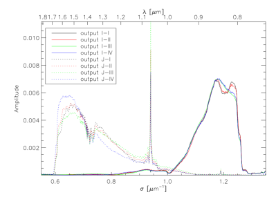
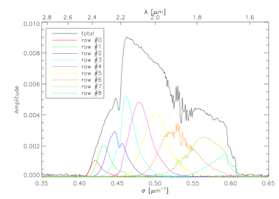
Figure 1: Left: Spectrum of the two spectral bands of the FS, which have two spectral bands over 4 outputs. Right: Spectra of the nine channels of the science camera, each one spread on two pixels on the detector.

Figure 1 presents the spectra of the FS bands and the science path. On the FS spectrum, we can see the pump laser of the supercontinuum source, at 1064 nm, and the absorption of the water vapor around 1.4 ¯m. The four outputs of each FS spectral band are slightly different. That effect deteriorate the linearity of the FS, especially on the J band. On the camera spectrum, we can see that the different channels are not equal, in intensity and bandwidth. The absorption of water vapor around 1.8 ¯m is also visible. With this analysis, we can deduce the central wavelength and the bandwidth of each channel.

3.2 Calibration of the density

We have three optical densities on the scientific spectral band, but they were not calibrated by the manufacturer, who did not have the appropriate instruments in this spectral band. The theoretical absorbance of those densities are 3, 4 and 5. So the idea is to calibrate the densities together, to reduce the contrast between measurements. So we compared density 3 with 4, 3 with 5, and 3+4 with 5. The needed contrast is then $10^{2}$, which is much less than the camera limit of $10^{4}$.

3.3 Calibration of the actuators

It consists in calibrating the PZT actuators of the two active M₆ mirrors. Each one has three piezoelectric motors, which allow movements in piston and tip/tilt. This calibration process measures the interaction matrix and computes its generalized inverse to derive the command matrix. The interaction matrix $\mathbf{M}_{int}$ is obtained by sending known commands (voltage ramps) to each piezo motor, and by measuring the slope on each axis on the Field Relative Angle Sensor (FRAS). The matrix $\mathbf{M}_{int}$ is then defined by

$$\begin{pmatrix}\frac{\displaystyle\mathrm{d}x}{\displaystyle\mathrm{d}t}\\[6.0pt] \frac{\displaystyle\mathrm{d}y}{\displaystyle\mathrm{d}t}\end{pmatrix}=\mathbf{M}_{int}\begin{pmatrix}\frac{\displaystyle\mathrm{d}V_{1}}{\displaystyle\mathrm{d}t}\\[6.0pt] \frac{\displaystyle\mathrm{d}V_{2}}{\displaystyle\mathrm{d}t}\\[6.0pt] \frac{\displaystyle\mathrm{d}V_{3}}{\displaystyle\mathrm{d}t}\end{pmatrix}.$$ (6)

We perform then a Singular Value Decomposition (SVD) to derive the inverse. The piston mode is not seen by the FRAS but can be reconstructed from a geometric model of the actuators, and its control added in the command matrix, which transforms commands in piston and tip/tilt to voltages to be sent on the 3 piezos 120˚apart in azimuth.

3.4 Calibration of the tip/tilt reference position

The purpose of this calibration is to obtain the reference position of the M₆ mirrors to inject a maximum flux in the single-mode fiber that guides the flux from the output III of the MMZ to the scientific camera. A sequential scan of each mirror is performed to move the focal spot in front of the fiber; the signal is synchronously acquired and is used to reconstruct an image. The theoretical intensity can be approximated by a gaussian function[16]:

$$I(\alpha,\beta)\simeq I_{inj,max}\exp\left[-\frac{\pi^{2}}{5}\sigma^{2}D^{2}\left((\alpha-\alpha_{ref})^{2}+(\beta-\beta_{ref})^{2}\right)\right],$$ (7)

with $I_{inj,max}$ the maximum injected flux, $D$ the diameter of the beam, $\alpha$ and $\beta$ the angles of tip and tilt, and $\alpha_{ref}$ and $\beta_{ref}$ the reference position which maximizes the injected flux.

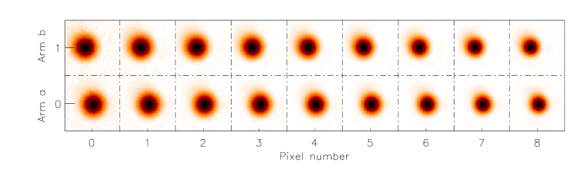
Figure 2: Reconstruction of the convolution of the PSF and the fundamental guidance mode of the single-mode fiber, for each spectral channel of the science camera.

The result of that reconstruction is shown in Fig. 2, for each channel of the science camera. We get a spot corresponding to the convolution of the PSF for each spectral channel with the fundamental guidance mode of the single-mode fiber. According to Eq. (7), the diameter of the spot is proportionnal to $\lambda$. This can be seen in Fig. 2: the diameter of the spot decreases as the wavelength decreases (left to right). We compute the centers of gravity for the two arms, which give the offsets to be applied to both mirrors. As the spots are centro-symmetric, this position corresponds to the maximum injection flow of each arm in the fiber. The dispersion of the centers of gravity for the different channels are negligible, so there is no chromatism in the reference position in tip/tilt.

3.5 Calibration of the fringe sensor

That procedure has already been described in Ref. 13. Since then it encountered a few changes, but the idea remains the same: we inject an OPD ramp with the M₆ actuators, to measure the phase shifts between the 4 outputs of the MMZ on the two spectral bands. Then we measure sequentially the flux on each arm, and the dark current of each detector. We have then the matrix $\mathbf{M}_{FS}$ given by the relation

$$\begin{pmatrix}I_{I}\\[2.0pt] I_{II}\\[2.0pt] I_{III}\\[2.0pt] I_{IV}\end{pmatrix}=\mathbf{M}_{FS}\begin{pmatrix}I_{a}\\[2.0pt] I_{b}\\[2.0pt] 2\mu\mathrm{Env}(\delta)\mathchoice{{\hbox{$\displaystyle\sqrt{I_{a}I_{b}\,}$}\lower 0.4pt\hbox{\vrule height=6.83331pt,depth=-5.46667pt}}}{{\hbox{$\textstyle\sqrt{I_{a}I_{b}\,}$}\lower 0.4pt\hbox{\vrule height=6.83331pt,depth=-5.46667pt}}}{{\hbox{$\scriptstyle\sqrt{I_{a}I_{b}\,}$}\lower 0.4pt\hbox{\vrule height=4.78333pt,depth=-3.82668pt}}}{{\hbox{$\scriptscriptstyle\sqrt{I_{a}I_{b}\,}$}\lower 0.4pt\hbox{\vrule height=3.41666pt,depth=-2.73334pt}}}\cos(2\pi\sigma\delta)\\[2.0pt] 2\mu\mathrm{Env}(\delta)\mathchoice{{\hbox{$\displaystyle\sqrt{I_{a}I_{b}\,}$}\lower 0.4pt\hbox{\vrule height=6.83331pt,depth=-5.46667pt}}}{{\hbox{$\textstyle\sqrt{I_{a}I_{b}\,}$}\lower 0.4pt\hbox{\vrule height=6.83331pt,depth=-5.46667pt}}}{{\hbox{$\scriptstyle\sqrt{I_{a}I_{b}\,}$}\lower 0.4pt\hbox{\vrule height=4.78333pt,depth=-3.82668pt}}}{{\hbox{$\scriptscriptstyle\sqrt{I_{a}I_{b}\,}$}\lower 0.4pt\hbox{\vrule height=3.41666pt,depth=-2.73334pt}}}\sin(2\pi\sigma\delta)\end{pmatrix},$$ (8)

with $I_{a}$ and $I_{b}$ are the flux of the two arms and $\mu\mathrm{Env}(\delta)$ the fringes envelope. The matrix $M_{FS}$ is inverted, to obtain the demodulation matrix D.

3.6 Calibration of the science camera

The calibration of the camera is made along with the calibration of the FS. Therefore, it uses the same sequence: an OPD ramp, the flux in each arm, and the dark current. With those information, we can analyze a few parameters, and compute the coefficient $\gamma$ of Eq. (2) for the calculation of the null rate.

With the data flux of arms $a$ and $b$, $I_{a}$ and $I_{b}$, we can estimate the photometric unbalance $\varepsilon$ by

$$\varepsilon=\frac{\left\langle I_{b}\right\rangle_{t}-\left\langle I_{a}\right\rangle_{t}}{\left\langle I_{b}\right\rangle_{t}+\left\langle I_{a}\right\rangle_{t}}.$$ (9)

As $I_{max}=(1+V)(I_{a}+I_{b})$, with the contrast $V\simeq 1$, then $I_{max}\simeq 2(I_{a}+I_{b})$; we estimate the coefficient $\gamma_{i}$ for each spectral channel by

$$\gamma_{i}=\frac{\left\langle I_{ref,i}\right\rangle_{t}}{2\left(\left\langle I_{a,i}\right\rangle_{t}+\left\langle I_{b,i}\right\rangle_{t}\right)}.$$ (10)

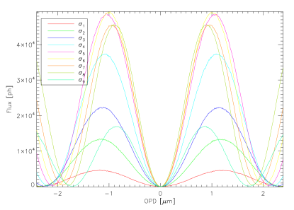
Figure 3: Interferogram acquired during the calibration of the camera.

Figure 3 presents an interferogram obtained on the camera during the OPD ramp of the calibration. We can see that every channel has different wavelengths, but their minima are at the same position. With those data, we can use a FTS mode, to determine the central frequency $f_{i}$ and the phase $\phi_{i}$ of each sinusoid.

With the frequency $f_{i}$, we can determine the wave number $\sigma_{i}$ with the slope of the OPD ramp $v$: $\sigma_{i}=f_{i}/v$. With the phase $\phi_{i}$, we can determine the position of the minimum of each sinusoid, by

$$\delta_{i}=\delta_{ref}+\frac{\phi_{i}}{2\pi\sigma_{i}},$$ (11)

with $\delta_{ref}$ is the reference position of the FS.

3.7 Correction of the tip/tilt reference position

When the temperature drifts, the reference position of the FRAS also drifts. This shift is usually small, so it is not necessary to repeat the procedure described above. A more efficient procedure has been developed for this purpose. It is inspired by the procedure of correction of the OPD position described below, called dithering[18].

Close to the reference position, we can approximate the exponential term of Eq. (7) with a quadratic term:

$$I(\alpha,\beta)\simeq I_{inj,max}\left(1-\frac{\pi^{2}}{5}\sigma^{2}D^{2}\left[(\alpha-\alpha_{ref})^{2}+(\beta-\beta_{ref})^{2}\right]\right)$$ (12)

For the two arms, for both axis, we put a small angle $\theta=6$ arcsec (11% of the Airy disk), and we measure the flux injected in the fiber. If $\alpha_{0}$ and $\beta_{0}$ are the current positions, we note $I_{0}=I(\alpha_{0},\beta_{0})$, $I_{\alpha_{-}}=I(\alpha_{0}-\theta,\beta_{0})$, $I_{\alpha_{+}}=I(\alpha_{0}+\theta,\beta_{0})$, $I_{\beta_{-}}=I(\alpha_{0},\beta_{0}-\theta)$ and $I_{\beta_{+}}=I(\alpha_{0},\beta_{0}+\theta)$.

Then, we calculate the reference position with

$$\left\{\begin{array}[]{rcl}\alpha_{ref}&=&\alpha_{0}-\frac{\displaystyle I_{\alpha_{+}}-I_{\alpha_{-}}}{\displaystyle 2\left(I_{\alpha_{+}}+I_{\alpha_{-}}-2I_{0}\right)}\cdot\theta\\[12.0pt] \beta_{ref}&=&\beta_{0}-\frac{\displaystyle I_{\beta_{+}}-I_{\beta_{-}}}{\displaystyle 2\left(I_{\beta_{+}}+I_{\beta_{-}}-2I_{0}\right)}\cdot\theta\\ \end{array}\right..$$ (13)

This procedure was successfully implemented on the bench, and showed a very good accuracy ($\approx 50$ mas, 0.1% of the Airy disk).

3.8 Correction of the OPD reference position

Despite the calibration procedure of the camera described above, the accuracy is not enough to guaranty a sub-nanometer positioning of the OPD to minimize the null rate. That position is also very sensitive to temperature variations. To correct the reference position of the FS $\delta_{ref}$, we use the technique of dithering[18].

The null rate has a quadratic dependence with the OPD[4]:

$$N(\delta)=N_{min}+(\pi\sigma(\delta-\delta_{ref}))^{2},$$ (14)

So we measure the null rate for three positions of OPD: the current position $\delta_{0}$, and two other positions $\delta_{0}-\varepsilon$ and $\delta_{0}+\varepsilon$, with $\varepsilon=2$ nm. If we note $N_{0}=N(\delta_{0})$, $N_{-\varepsilon}=N(\delta_{0}-\varepsilon)$ and $N_{+\varepsilon}=N(\delta_{0}+\varepsilon)$, the reference position is then

$$\delta_{ref}=\delta_{0}-\frac{N_{+\varepsilon}-N_{-\varepsilon}}{2\left(N_{+\varepsilon}+N_{-\varepsilon}-2N_{0}\right)}\cdot\varepsilon$$ (15)

That reference position is very sensitive to temperature variations, about 600 nm.K^-1. However, we consider that temperature variations over 100 s are less than 1 mK in normal conditions, so the thermal drift is less than 0.6 nm over 100 s.

4 LQG EXPERIMENTAL VALIDATION

PERSEE aims to simulate a nulling space mission, constituted of three satellites: two siderostats and a central combiner. The three satellites are controlled by impulsive gas thrusters and reaction wheels, from individual star trackers, a radiofrequency metrology, optical lateral metrology and off-loading signals from the central combiner. Those systems lead to different types of disturbances, viz., microvibrations due to the reaction wheels, linear-parabolic drift due to the solar pressure and the gas impulses, and low-frequency pointing control (PC) residue.

Vibrations are the main disrupters of the OPD, which are not always well corrected by an integrator in a control loop. We implemented the method described in Ref. 13, based on the work for the extreme adaptive optics instrument SPHERE at Onera[19]. It is based on a Linear Quadratic Gaussian (LQG) control law that provides an optimal correction of vibrations, in the sense of residual phase minimum variance.

4.1 Identification of the pointing control residue and vibration filtering efficiency

In a first test, we analyze the correction of the PC residue, with a classical integrator and a LQG.

We note $\sigma_{OL,dis}^{2}$ the open-loop OPD variance for a case where we inject a PC residue of variance $\sigma_{inj,PC}^{2}$, and vibrations of variance $\sigma_{inj,vib}^{2}$. If $\sigma_{OL,exp}^{2}$ is the open-loop OPD variance of the experiment without any injected disturbance, then

$$\sigma_{OL,dis}^{2}=\sigma_{OL,exp}^{2}+\sigma_{inj,PC}^{2}+\sigma_{inj,vib}^{2}.$$ (16)

So if $\sigma_{OL,PC}^{2}$ is the open-loop OPD variance for the case where we inject only PC residue, we have $\sigma_{OL,PC}^{2}=\sigma_{OL,exp}^{2}+\sigma_{inj,PC}^{2}$, and then $\sigma_{OL,dis}^{2}=\sigma_{OL,PC}^{2}+\sigma_{inj,vib}^{2}$.

For this test, we compute the following power residue percentage

$$\rho_{c,PC}=\frac{\sigma_{c,PC}^{2}-\sigma_{c,exp}^{2}}{\sigma_{OL,PC}^{2}-\sigma_{c,exp}^{2}},\ c\in\{int,LQG\},$$ (17)

with $\sigma_{c,exp}^{2}$ the residual OPD variance for the controller $c$ (integrator or LQG) when we do not inject disturbances, and $\sigma_{c,PC}^{2}$ the same quantity for the case where we inject the PC residue. In that case, if $\sigma_{c,PC}^{2}=\sigma_{c,exp}^{2}$, then $\rho_{c,PC}=0$%, the injected disturbance is totaly corrected, and if $\sigma_{c,PC}^{2}=\sigma_{OL,PC}^{2}$, then $\rho_{c,PC}=100$%, the controller has no effect.

POINTING CONTROL RESIDUE CORRECTION
Controller $c$	$\sigma_{c,PC}$	$\rho_{c,PC}$
Integrator	0.45 nm rms	0.17%
LQG	0.37 nm rms	0.09%

Table 1: Correction of the PC residue with the integrator and the LQG.

Numerical results of the two controllers are presented in Tab. 1. With that type of disturbance, i.e. with a continuously decreasing spectrum like in AO with turbulence, the integrator and the LQG have similar performance: the power residue is very low in each case, with a slight improvement from the LQG.

For the following tests, we will compute a vibration residue percentage, similar to the one used in Ref. 19:

$$\rho_{c}=\frac{\sigma_{c,dis}^{2}-\sigma_{c,PC}^{2}}{\sigma_{OL,dis}^{2}-\sigma_{OL,PC}^{2}-\sigma_{c,PC}^{2}},\ c\in\{int,LQG\}$$ (18)

with $\sigma_{c,dis}^{2}$ is the residual OPD variance for the controller $c$ for the case where we inject the PC residue with vibrations.So if $\sigma_{c,dis}^{2}=\sigma_{c,PC}^{2}$, the $\rho_{i}=0$%, the vibrations are totally removed. On the contrary, if $\sigma_{c,dis}^{2}=\sigma_{inj,vib}^{2}$, $\rho_{c}=100$%, the vibrations are not corrected.

4.2 Experimental correction of a single vibration

In those tests, we inject the PC residue with one vibration, at several frequencies, and we compare the correction of the integrator and the LQG.

CORRECTION OF A SINGLE VIBRATION
$f_{vib}$	$\sigma_{int,dis}$	$\rho_{int}$	$\sigma_{LQG,dis}$	$\rho_{LQG}$
[Hz]	[nm rms]	[%]	[nm rms]	[%]
1.1	0.49	0.08	0.38	0.02
2.2	0.58	0.34	0.40	0.06
5.5	0.87	1.2	0.47	0.17
11	1.5	8.9	0.38	0.03
22	3.0	17	0.52	0.27
55	7.1	92	0.65	0.53
110	11	220	0.4	0.04
220	4.4	130	0.38	0.04

Table 2: Correction of single vibrations at different frequencies.

Table 2 presents the results of the integrator and the LQG for different vibration frequencies. As expected, the correction of the integrator deteriorates as the frequency increases, in contrast to LQG, which maintains a fairly constant performance $\rho_{LQG}$ close to 0%.

For $f_{vib}=1.1$ and 2.2 Hz, the injected vibration was not identified, but corrected as a part of the PC residue contribution (the continuum part); it does not affect the result of the correction: the disturbance is totally removed.

Table 2 shows that after 22 Hz, for 10 nm vibrations, the integrator is not efficient to correct the disturbances at the required level of 1.8 nm rms. Also, the power of the vibration at 110 Hz is doubled, because of the overshoot in the integrator closed-loop transfer function.

These tests revealed a limitation of identification: the spectral resolution of the FFT. Indeed, if a sinusoid has not an integer number of periods in the signal supplied to the identification, the fitted vibration will have a damping factor greater than reality.

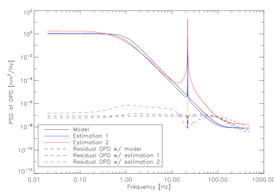
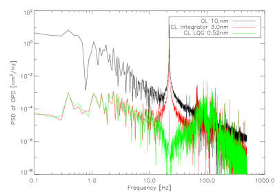
Figure 4: Frequency evolution of the identification, and on the residual OPD (simulation and experimental results).

Figure 4 illustrates that effect. In that example, the model used is a typical PC residue, with a single vibration around 22 Hz (black solid line). For the estimation 1 (blue solid line), the vibration has an integer number of periods in the time sequence used for identification. The estimation is then close to the model for the PC residue, and the identified damping coefficient for the vibration is $10^{-5}$. Then the OPD residue is close to the ideal one, giving almost a white noise. For the estimation 2 (red solid line), the number of periods is not aninteger, the peak maximum is between two points of the periodogram. In that case, because of the contrast between the vibration and the PC residue, the peak is not sharp, but has some leakages around the central frequency. The identification is degraded, the PC residue is not perfectly fitted, especially at the cutoff frequency. For the vibration, the identification gives a greater damping coefficient of $5\times 10^{-4}$, and a reduced amplitude. On the OPD residue, we can see that the signal is overcorrected around the vibration frequency, while the vibration is not perfectly suppressed. This overcorrection is compensated by a higher residue at low frequencies.

4.3 Experimental correction of realistic disturbances

These tests aim to simulate as accurately as possible the conditions of disturbance of a space mission. To do so, we consider two levels of PC residue: an optimistic value of 3 nm rms, and a conservative value of 15 nm rms.

Added to that residue, we also inject the characteristic vibrations of 6 reaction wheels, rotating at different frequencies, close to a central frequency $f_{rw}$. We consider three rotation frequencies, 1.5, 3 and 4.5 Hz, corresponding to typical GNC design values. Those reaction wheels generate a set of vibrations, related to the first harmonic of the wheel.

No detailed mechanical model was available, and the following assumptions were made from typical satellite behavior known at CNES. Some of the frequencies are amplified by structure modes in the satellites: a mode of sunshade at 15 Hz, a fundamental lateral mode of the satellite at 55 Hz, and local modes of the wheel cavity and the optics at 75 and 85 Hz.

Those parameters lead to six different cases that are studied with a simple simulator of the bench, and compared to experimental results. For a central frequency $f_{rw}=1.5$ Hz, only the first harmonics are significant, no harmonic is amplified by the structure modes. For $f_{rw}=3$ Hz, some harmonics are amplified at 55 Hz, while for $f_{rw}=4.5$ Hz, harmonics are also amplified at 75 and 85 Hz.

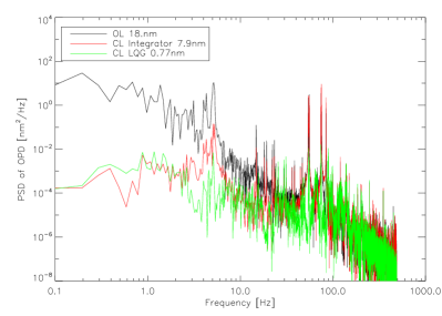
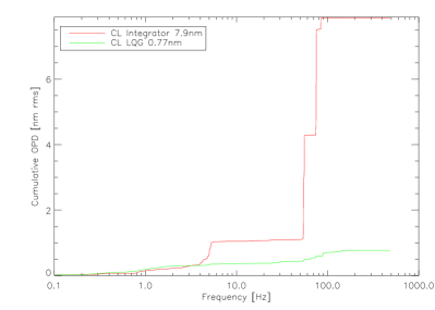
Figure 5: PSD and cumulative OPD for the correction of realistic disturbance, with an integrator and a LQG. The parameters of the disturbance are $f_{rw}=4.5$ Hz and $\sigma_{OL,PC}=15$ nm rms.

Figure 5 presents the correction of the worst studied case: $f_{rw}=4.5$ Hz and $\sigma_{OL,PC}=15$ nm rms. For the LQG, the identification is made on the 20 strongest vibrations. We set the integrator gain at 0.5.

COMPARISON B/W SIMULATIONS AND EXPERIMENTS
$f_{rw}$	$\sigma_{OL,PC}$	$\sigma_{int,dis}$	$\rho_{int}$	$\sigma_{LQG,dis}$	$\rho_{LQG}$
[Hz]	[nm rms]	[nm rms]	[%]	[nm rms]	[%]
1.5	3	0.62	0.54	0.41	0.09
1.5	15	0.58	0.06	0.44	0.03
3.0	3	2.2	11	0.47	0.20
3.0	15	4.8	13	0.51	0.07
4.5	3	4.3	58	0.49	0.34
4.5	15	7.9	22	0.77	0.17

Table 3: Influence of the number of vibrations.

Table 3 presents the comparison between the simulations and the experimental results for the 6 different cases. We can see that the integrator can manage the disturbance at the required levels for $f_{rw}=1.5$ Hz, whatever the level of RF PC residue. For those cases, the LQG gives a substantial improvement, leading to a nulling contribution divided by 2. The interest of LQG is more significant for the other cases, because amplified harmonics are not properly corrected by the integrator. As expected, the LQG corrector removes almost the whole power of the disturbance.

5 NULLING ANALYSIS

5.1 Nulling calculation and contributors

On PERSEE, we carry out a spectral analysis of the null rate, so we analyze separately the different spectral channels. Thus, we calculate an average null rate over the entire band, rather than an integrated null rate, which is more dependant of the spectrum. Therefore, the spectral bandwidth is larger.

With the result of Fig. 1, we calculate the spectral widths $\left(\frac{\Delta\sigma}{\sigma}\right)_{i}$ for each channel $i$. Then the total spectral bandwidth is deduced from the extreme channels:

$$\Delta\sigma_{m}=\sigma_{n}+\frac{\Delta\sigma_{n}}{2}-\sigma_{1}+\frac{\Delta\sigma_{1}}{2},$$ (19)

with $n$ the number of channel ($n=9$). Then, the total bandwidth is $\left(\frac{\Delta\sigma}{\sigma}\right)_{m}=37$% around the central wave number $\sigma_{m}=0.5$ ¯m^-1, i.e. a central wavelength $\lambda_{m}=2.0$ ¯m. For the analysis of the bench performance, we will then compute the mean null rate $N_{m}=\left\langle N_{i}\right\rangle_{i}$.

The null rate can be decomposed in a sum of independent contributors[17]:

$$N_{m}(t)=\frac{1}{4}\left[\Delta\phi_{c}(t)^{2}+\left\langle\Delta\phi_{\lambda}(t)^{2}\right\rangle_{t}+\frac{\pi^{2}}{4}\left(\theta_{dia}\sigma_{max}b\right)^{2}+\frac{1}{4}(\Delta\phi_{s-p})^{2}+\alpha^{2}_{rot}+\varepsilon(t)^{2}\right],$$ (20)

where:

• $\Delta\phi_{c}(t)$ is the phase fluctuation at the central wavelength, while $\Delta\phi_{\lambda}(t)$ takes into account the chromatic dispersion of the null;

• $\theta_{dia}$ is the angular diameter of the source, $\sigma_{max}$ the maximum wavenumber of the spectrum and $b$ the interferometric baseline;

• $\Delta\phi_{s-p}$ is the phase difference between the two polarizations $s$ et $p$, and $\alpha_{rot}$ is the rotation angle of the polarization $s$ (or $p$) between the two beams of the interferometer;

• $\varepsilon(t)$ are the fluctuations of intensity mismatch, defined by $\varepsilon=\frac{I_{b}-I_{a}}{I_{b}+I_{a}}$, with $I_{a}$ and $I_{b}$ the flux on the arms $a$ and $b$.

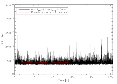
Figure 6: Best result of null rate on 100 s: temporal sequence of the mean null rate (left) and temporal average of the null rates on the different spectral channels (right).

Figure 6 presents the best result obtained on the bench, on a 100 s timescale, with an acquisition frequency of 100 Hz, and an integration time of 2.58 ms. The mean value is

$$\left\langle N_{m}\right\rangle_{t=100s}=8.9\times 10^{-6}.$$

The standard deviation $\sigma_{N,T}$ depends on the integration time $T$. We chose to consider $T=1$ s, more representative of a real mission. Then, we have $\sigma_{N,T=2.58\mathrm{ms}}=1.8\times 10^{-6}$ and $\sigma_{N,T=1\mathrm{s}}=2.7\times 10^{-7}$. The chromatic dispersion of the null rate is between $6.9\times 10^{-6}$ and $1.58\times 10^{-5}$ on the spectrum. the degradation of the null rate at short wavelengths is explained by both OPD and flux mismatch effects, but the degradation of the highest wavelength is probably due to polarization effects.

5.2 OPD fluctuations and chromatism

The OPD fluctuations are an important contribution of the null rate. The different spectral channels are disturbed differently by the OPD fluctuations.

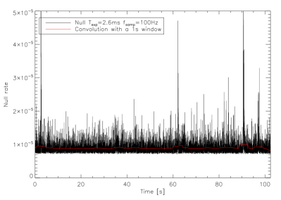
Figure 7: Simulation of the null rate (left) with the measured OPD (right).

Figure 7 presents the contribution of the OPD on the mean null rate. Compared to Fig. 6, we can see exactly the same disturbances, with a similar amplitude. The OPD disturbances are characterized by their standard deviation $\sigma_{OPD}=0.80$ nm rms. According to Eq. 20, the contribution of the OPD on the null rate is then

$$N_{\delta}=\pi^{2}\left\langle\sigma_{i}^{2}\right\rangle_{i}\left\langle(\delta-\delta_{m})^{2}\right\rangle_{t},\text{ with }\delta_{m}=\frac{\left\langle\sigma_{i}^{2}\delta_{i}\right\rangle_{i}}{\left\langle\sigma_{i}^{2}\right\rangle_{i}}.$$ (21)

That contribution can be reduced by having $\delta_{ref}=\delta_{m}$, especially with the calibration described in Sec. 3.8. But for this case, the calibration was not operationnal, so the search of the optimal $\delta_{ref}$ was made manually.

So the contribution of OPD fluctuations and static error are

$$N_{\delta}=\pi^{2}\left\langle\sigma_{i}^{2}\right\rangle_{i}\left(\delta_{ref}^{2}+\sigma_{OPD}^{2}\right)$$ (22)

In this case, we measured $|\delta_{ref}|=0.48$ nm. So the OPD contribution is $N_{\delta}=1.7\times 10^{-6}$. We can also calculate the contribution of the null rate stability $\sigma_{N,\delta,T}$: we have $\sigma_{N,T=2.58\mathrm{ms}}=1.8\times 10^{-6}$ and $\sigma_{N,T=1\mathrm{s}}=3.1\times 10^{-7}$. Those values are almost equal to the stability of the null rate, which shows that the null rate is only disturbed by the OPD variations.

The reference position of the FS does not optimize the null rate of each spectral channel, because of the phase dispersion $\left\langle\Delta\phi_{\lambda}(t)\right\rangle_{t}$. That dispersion is measured during the correction of the OPD reference position presented in Sec. 3.

The contribution of the chromatism to the null rate, is then [17]

$$N_{\lambda,i}=(\pi\sigma_{i}(\delta_{i}-\delta_{ref}))^{2}.$$ (23)

So the total contribution on the whole spectral band is

$$N_{\lambda}=\pi^{2}\left\langle(\sigma_{i}(\delta_{i}-\delta_{ref}))^{2}\right\rangle_{i}.$$ (24)

Figure 8: Chromatic dispersion of the positions of best null rates for the channels of the camera, and its contribution to the null rate.

Figure 8 presents a measurement of the chromatic dispersion on the channels of the camera. The contribution of the chromatism, calculated with Eq. (24), is then $N_{\lambda}=4.6\times 10^{-7}$. This chromatism is due to the beam splitters of the MMZ, especially the thickness differences of both plates and coatings, and also the difference in incidence angle between the two arms.

5.3 Stellar leakage

The contributor corresponding to stellar leakage $N_{*}$ , corresponds in Eq. (20) to

$$N_{*}=\frac{\pi^{2}}{16}(\theta_{dia}\sigma_{max}b)^{2}.$$ (25)

The angular diameter $\theta_{dia}$ of the source is given by the ratio of the diameter of the fiber $d$ and the focal length $f_{0}$ of the collimator. On PERSEE, $d=4.3$ ¯m and $f_{0}=750$ mm, $b=50$ mm and $\sigma_{max}=0.61$ ¯m^-1, So the stellar leakage would be $N_{*}=1.9\times 10^{-2}$.

However, we obtained much better null rate. Indeed, this calculation applies only for a spatially incoherent source, whereas in the case of PERSEE, the source is spatially coherent, due to the single-mode fiber. Therefore, there is no stellar leakage.

5.4 Photometric mismatch

The contribution of the photometric mismatch depends on the tip/tilt residue of the control-loop, and the static photometric mismatch of the instrument.

From the Equation (12), we can write

$$\left\{\begin{array}[]{rcl}I_{a,i}&=&I_{a,i,max}(1-\frac{\displaystyle\pi^{2}}{\displaystyle 5}\sigma_{i}^{2}D^{2}\zeta_{a}^{2})\\[6.0pt] I_{b,i}&=&I_{b,i,max}(1-\frac{\displaystyle\pi^{2}}{\displaystyle 5}\sigma_{i}^{2}D^{2}\zeta_{b}^{2})\\ \end{array}\right.,$$ (26)

with $\zeta_{a}^{2}=(\alpha_{a}-\alpha_{a,ref})^{2}+(\beta_{a}-\beta_{a,ref})^{2}$ and $\zeta_{b}^{2}=(\alpha_{b}-\alpha_{b,ref})^{2}+(\beta_{b}-\beta_{b,ref})^{2}$.

Then the photometric mismatch $\varepsilon_{i}$ on each channel $i$ is

$$\varepsilon_{i}=\varepsilon_{stat,i}+\frac{\pi^{2}}{10}\sigma_{i}^{2}D^{2}(\zeta_{a}^{2}-\zeta_{b}^{2}),$$ (27)

with $\varepsilon_{stat,i}=\frac{\displaystyle I_{b,i,max}-I_{a,i,max}}{\displaystyle I_{b,i,max}+I_{a,i,max}}$. Then the contribution of photometric mismatch on each channel is

$$N_{\varepsilon,i}=\frac{\varepsilon_{stat,i}^{2}}{4}+\frac{\pi^{4}}{400}\sigma_{i}^{4}D^{4}(\zeta_{a}^{2}-\zeta_{b}^{2})^{2}.$$ (28)

The contribution on the null rate is then

$$N_{\varepsilon}=\frac{\left\langle\varepsilon_{stat,i}^{2}\right\rangle_{i}}{4}+\frac{\pi^{4}}{400}D^{4}\left\langle\sigma_{i}^{4}\right\rangle_{i}(\zeta_{a}^{2}-\zeta_{b}^{2})^{2}$$ (29)

Figure 9: Photometric mismatch on the different channels of the camera.

The static contribution of the photometric mismatch $\varepsilon_{stat,i}$ is calculated during the calibration of the camera, and is only due to the instrument optics. Figure 9 presents a measurement of $\varepsilon_{stat}$, and its contribution on the null rate, calculated by

$$N_{\varepsilon,stat,i}=\frac{\varepsilon_{stat,i}^{2}}{4}.$$ (30)

Thus, the total contribution of instrumental photometric mismatch is given by

$$N_{\varepsilon,stat}=\frac{\left\langle\varepsilon_{stat,i}^{2}\right\rangle_{i}}{4}.$$ (31)

That contribution is then $N_{\varepsilon,stat}=3.9\times 10^{-6}$.

The residue of tip/tilt control is also measured, and has a typical standard deviation $\sigma_{tip/tilt,axis}=56$ mas rms on each axis, so the stability of the position on each arm is $\sigma_{tip/tilt}=80$ mas rms (0.14% of the Airy disk).

According to Eq. (29), the dynamic contribution of the control loop residue to the null rate is

$$N_{\varepsilon,dyn}=\frac{\pi^{4}}{100}D^{4}\left\langle\sigma_{i}^{4}\right\rangle_{i}\sigma_{tip/tilt}^{4}.$$ (32)

Then, that contribution is $N_{\varepsilon,dyn}=1.1\times 10^{-11}$. It is clearly negligible compared to $N_{\varepsilon,stat}$, but the relation in $\sigma_{tip/tilt}^{4}$ is very sensitive to the FRAS correction residue.

For the stability over 100 s, the contribution of the tip/tilt control loop is very faint, at $\sigma_{N,tip/tilt,T=1\mathrm{s}}=1.4\times 10^{-12}$, a few decades under the contribution of the OPD control loop.

5.5 Polarization study

We have no way to measure the polarization contributions, but we can estimate them from subtracting the other known contributions, by the equation:

$$N_{pol}=N_{m}-N_{\delta}-N_{\lambda}-N_{\varepsilon}$$ (33)

So, with $N_{m}=8.9\times 10{-6}$, $N_{\delta}=1.7\times 10^{-6}$, $N_{\lambda}=4.6\times 10^{-7}$ and $N_{\varepsilon}=N_{\varepsilon,stat}=3.9\times 10^{-6}$, we can estimate the contribution of polarization effects at $N_{pol}=2.8\times 10^{-6}$.

So if that contribution is only attributed to the phase difference between the polarizations $s$ and $p$, the OPD difference between the two polarizations is $\delta_{s-p}=2.1$ nm. On the contrary, if the contribution is only comming from the angle of the polarizations of the two arms, that angle is $\alpha_{rot}=3.3$ mrad.

5.6 Stability of the null rate over 7 hours

We are currently conducting stability tests over a few hours (typically 10 h), the typical duration of a target observation during a space mission. The first test was made over 7 h during the night, with a sub-optimal alignment. The average null rate is then higher than the value analyzed above.

Figure 10: First measurement of null rate over 7 h: temporal sequence of the mean null rate (left) and temporal average of the null rates on the different spectral channels (right).

Figure 10 presents the first long-term measurement of the null rate over 100 s. We can see on the left figure that the null rate has a higher value than the best result: $\left\langle N_{m}\right\rangle_{T=7\mathrm{h}}=3.37\times 10^{-5}$, but shows a very good stability over 7 h: $\sigma_{N,T=100\mathrm{s}}=9\times 10^{-7}$. That measured stability is a decade better than the specification: $\sigma_{N,T=100\mathrm{s}}=10^{-5}$.

In Fig. 10 (right), the null rate spectral profile looks like the one presented in Fig. 6: the null rate is better at the center of the spectrum than at the edges. The contribution of OPD and flux mismatch are also higher at shorter wavelengths, and the contribution of polarization should be higher at longer wavelengths. The chromatic dispersion of the null rate is between $1.3\times 10^{-5}$ and $8.7\times 10^{-5}$, so the amplitude is 7 times higher than on the best result.

OVERVIEW OF NULL RATE ANALYSIS
Contribution	Specification	Best null (100 s)	Null rate (7 h)
$\left\langle N_{m}\right\rangle_{t}$	$10^{-4}$	$8.9\times 10^{-6}$	$3.37\times 10^{-5}$
$N_{\delta}$	$3.5\times 10^{-5}$	$1.7\times 10^{-6}$	$2.8\times 10^{-6}$
$N_{\lambda}$	$3.5\times 10^{-5}$	$4.6\times 10^{-7}$	$5.4\times 10^{-6}$
$N_{\varepsilon}$	$2\times 10^{-5}$	$3.9\times 10^{-6}$	$3.3\times 10^{-6}$
$N_{pol}$	$10^{-5}$	$2.8\times 10^{-6}$	$2.2\times 10^{-5}$
$\sigma_{N,T=1\mathrm{s}}$	$1.5\times 10^{-5}$	$3\times 10^{-7}$	$2\times 10^{-7}$
$\sigma_{N,\delta,T=1\mathrm{s}}$	$1.5\times 10^{-5}$	$3\times 10^{-7}$	$2\times 10^{-7}$
$\sigma_{N,\varepsilon,T=1\mathrm{s}}$	$3\times 10^{-6}$	$1.4\times 10^{-12}$	$1.5\times 10^{-11}$
$\sigma_{N,T=100\mathrm{s}}$	$10^{-5}$	-	$9\times 10^{-7}$

Table 4: Overview of the analysis of the best null rate over 100 s and the null rate measured over 7 h, in average value and stability, and comparison with the original specifications of the bench.

Table 4 summarizes the null rate analysis developped in this section. In the near futur, we should be able to achieve an average null rate of $10^{-5}$ over 10 h, with a stability better than $10^{-6}$, i.e. a decade under the original specifications of the bench. As we also demonstrate the capability of correcting injected disturbances, we should be able to achieve that result even with typical disturbances on the bench.

6 CONCLUSION

PERSEE showed a very high quality and performance well beyond the initial specifications. The large majority of goals has already been demonstrated. We have already presented some important lessons in Ref. 13, about thermal stability and control loop feasibility. However, we can complete these remarks by other conclusions.

Firstly, we elaborated a calibration scheme that can be applied to a space mission, although it must take into account the linear-parabolic drift.That procedure is fully automatic, and allows also to make an accurate analysis of the instrument.

Secondly, we showed that a LQG controller can manage the disturbances of the OPD, to achieve a very deep null rate. An experimental sub-nanometer control has been demonstrated, even in the case of strong disturbances (more than 100 nm rms reduced to 1 nm rms). That result was very important for PERSEE, because we work in the near infrared, which is more sensitive to OPD variations than thermal infrared used in projects like DARWIN.

Finally, we showed that thanks to a a very efficient design, we obtained null rates more than 10 times better than the initial conservative goal of $10^{-4}$, thus close to the requirement of a nuller for the observation of telluric planets. We achieved the deepest null ever achieved by a near-infrared nulling interferometer: $8.9\times 10^{-6}$ on a 37% bandwidth, between 1.65 and 2.45 ¯m. PERSEE bench shows also a very good stability over 100 s, and also over 7 hours. We still have to confirm this deep null rate over 10 hours, with the same type of stability, and with injected disturbances.

The last steps will be the correction of linear-parabolic drifts, together with the use of a new source module, which includes a planet and an exozodiacal disk, presented in Ref. 15 during this conference.

- [1] Léger, A., et al., “The DARWIN project,” Astrophysics and Space Science 241, 135-146 (1996).
- [2] Léger, A., et al., “DARWIN mission proposal to ESA,” ESA’s Cosmic Vision Call for Proposals, (2007).
- [3] Beichman, C. A., et al., “The Terrestrial Planet Finder (TPF) : a NASA Origins Program to search for habitable planets,” (1999).
- [4] Lawson, P. R., “Principles of Long Baseline Stellar Interferometry,” (2000).
- [5] Danchi, W. C., et al., “Scientific rationale for exoplanet characterization from 3-8 microns: the FKSI mission,” Proc. SPIE 6268, 626820 (2006).
- [6] Ollivier, M., et al., “Pegase, an infrared interferometer to study stellar environments and low mass companions around nearby stars,” ESA’s Cosmic Vision Call for Proposals, (2007).
- [7] Le Duigou, J.-M., “Pegase: A Free Flying Interferometer for the Spectroscopy of Giant Exo-Planets,” ESA Special Publication 621, (2006).
- [8] Cassaing, F., et al., “PERSEE: a nulling demonstrator with real-time correction of external disturbances,” Proc. SPIE 7013(1), 70131Z (2008).
- [9] Le Duigou, J.-M., et al., “First results of the PERSEE experiment,” Proc. ICSO, (2010).
- [10] Coudé du Foresto, V., et al., “ALADDIN: an optimized nulling ground-based demonstrator for DARWIN,” Proc. SPIE 6268, 626810 (2006).
- [11] Houairi, K., et al., “PERSEE, the dynamic nulling demonstrator: Recent progress on the cophasing system,” Proc. SPIE, 70131W (2008).
- [12] Jacquinod, S., et al., “PERSEE: description of a new concept for nulling interferometry recombination and opd measurement,” Proc. SPIE 7013, 70131T (2008).
- [13] Lozi, J., et al., “PERSEE: Experimental results on the cophased nulling bench,” Proc. SPIE 7734, 77342M (2010).
- [14] Hénault, F., et al., “Review of OCA activities on nulling testbench PERSEE,” Proc. SPIE 7734, 77342U (2010).
- [15] Hénault, F., et al., “Design of a star, planet and exo-zodiacal cloud simulator for the nulling testbench PERSEE,” Proc. SPIE 8151, 8151-41 (2011).
- [16] Ruilier, C., et al., “Coupling of large telescopes and single-mode waveguides: application to stellar interferometry,” JOSA A 18(1), 143-149 (2001).
- [17] Serabyn, E., et al., “Fully symmetric nulling beam combiners,” Appl. Opt. 40(10), 1668-1671 (2001).
- [18] Gabor, P., et al., “Stabilising a nulling interferometer using optical path difference dithering,” A&A 483(1), 365-369 (2008).
- [19] Meimon, S., et al., “Tip/tilt disturbance model identification for Kalman-based control scheme: application to XAO and ELT systems,” JOSA A 27(11), A122-A132 (2010).