Elementary excitations and the phase transition in the bimodal Ising spin glass model

Abstract

We show how the nature of the the phase transition in the two-dimensional bimodal Ising spin glass model can be understood in terms of elementary excitations. Although the energy gap with the ground state is expected to be $4J$ in the ferromagnetic phase, a gap $2J$ is in fact found if the finite lattice is wound around a cylinder of odd circumference $L$. This $2J$ gap is really a finite size effect that should not occur in the thermodynamic limit of the ferromagnet. The spatial influence of the frustration must be limited and not wrap around the system if $L$ is large enough. In essence, the absence of $2J$ excitations defines the ferromagnetic phase without recourse to calculating magnetisation or investigating the system response to domain wall defects. This study directly investigates the response to temperature. We also estimate the defect concentration where the phase transition to the spin glass glass state occurs. The value $p_{c}=0.1045(11)$ is in reasonable agreement with the literature.

I Introduction

Spin glasses BY86 ; MPV87 ; FH91 ; KH04 have attracted much interest for quite a while. Due to the considerable complexity of real materials much computational effort has gone into studies of a simplified model EA75 that is nevertheless thought to include the essential ingredients that lead to spin glass behaviour. Since even this model is not trivial, a considerable industry has developed over time devoted to particular models that, although probably unphysical, have provided subjects for the development of numerical techniques HR01 ; Hart09 .

Systems known as spin glasses are disordered magnetic systems characterised by a random mixture of ferromagnetic and antiferromagnetic exchange interactions leading to frustration Toulouse . Typically, at low temperatures below a critical temperature $T_{c}$, a system undergoes a phase transition from a ferromagnet to a spin glass at some critical concentration $p_{c}$ of antiferromagnetic interactions.

The model studied in this work is the bimodal, or $\pm J$, Ising spin glass in two dimensions. This system has quenched bond (short range, nearest neighbour) interactions of fixed magnitude $J$ but random sign. The concentration $p$ of negative, or antiferromagnetic, bonds is varied from zero up the canonical spin glass at $p=0.5$. It is believed that the spin glass can only exist at zero temperature ON09 where $p>p_{c}$ with WHP03 ; AH04 $p_{c}=0.103$. This is clearly below the concentration $p_{n}=0.109$ at the (finite temperature) Nishimori point, indicating a reentrant phase transition as confirmed by Monte Carlo work TPV09 .

The ground state is highly degenerate with an entropy per spin BGP98 ; LGM04 of $0.07k$. Consequently spin correlation functions are not guaranteed to take values $\pm 1.0$. If a nearest-neighbour bond correlation function does have a value $\pm 1.0$ then we call that bond a rigid bond BMR82 . This means that the spin alignment across the bond is the same in all ground state configurations. A recent study RRNRV10 suggests that the rigid lattice does not percolate in the spin glass phase. This is consistent with the idea that the ferromagnetic phase is characterised by percolation of rigid bonds.

Droplet theory McMillan84 ; BF86 ; FH86 ; BM87 ; FH88 has enjoyed much success with regard to understanding the spin glass phase. The essential idea is that reversing all the spins in a compact cluster with respect to a ground state provides a low energy excitation. Typical droplet excitations dominate the thermodynamic behaviour. A closely related idea is the domain wall defect McMillan84x ; BM84 ; essentially a droplet perimeter that extends to infinity. With a continuous distribution of disorder these related views seem to be equivalent HY02 according to the predictions of droplet theory.

For the bimodal model domain wall defects have, for example, been applied KR97 ; AH04 to the determination of the value of the critical defect concentration $p_{c}$. Nevertheless, it still remains unclear whether droplet theory is appropriate Hart08 . The ground state is not unique and a droplet may represent some different ground state; not an excitation.

For this study the $L\times L$ square lattice is wound around a cylinder, that is we use periodic boundary conditions in one dimension. In the second dimension the system is nested in an infinite unfrustrated environment. There are no open boundaries. If the circumference $L$ of the cylinder is even then the energy gap is $4J$. Otherwise it is $2J$. In the spin glass phase the distribution of degeneracies of the first excited state is extreme with a long tail representing large values DTWWTSC04 ; Wanyok . We have also looked at systems with open boundaries and have found extreme distributions of $2J$ excitations in some agreement with Wang WangWorm .

The issue of the size of the energy gap of the bimodal Ising spin glass dates back to the proposal of Wang and Swendsen WS88 that it should be $2J$ in the thermodynamic limit. It now seems clear that in fact there is no energy gap at all and the low temperature specific heat varies as a power law $c_{v}\sim T^{-\alpha}$. The first indications of this appeared in Ref. Jorg06, and confirmation THM11 from the evaluation of very large Pfaffians has recently appeared.

The issue that remains unclear is the value of the critical exponent $\alpha$. For the case of continuous (Gaussian) disorder, direct calculations Cheung83 ; HH04 report that the specific heat is linear with $\alpha=-1.0$. For bimodal disorder Monte Carlo work KLC07 reports that $\alpha=-4.21$ while droplet theory THM11 suggests that $\alpha=-3.0$ although the temperature range used is extremely narrow. Other Monte Carlo results Jorg06 ; KLC07 for the correlation length with the assumption of hyperscaling gives $\alpha=-7.1$. Universality is hard to prove.

The exponent $\alpha$ is difficult to estimate. One reason that makes this so for the bimodal case is that the specific heat is not normally distributed. We have performed some calculations with open boundaries and find that the distribution of the specific heat has a tail for low temperature and small values of linear sample size $L$. The methods used were direct evaluation of Pfaffians as well as summing the density of states SK93 . Although it is reasonable to believe that the specific heat will be normally distributed in the thermodynamic limit, it is not clear what value to use from calculations with finite $L$.

It is at least clear now that the low-temperature specific heat contains contributions from excitations having a range of energies. This fits well with droplet theory THM11 where it is predicted that $\alpha=1-2/\theta_{S}$ with the fractal dimension of domain walls given by $d_{f}=2\theta_{S}$. If $\theta_{S}=0.5$ as reported SK93 ; LMMS06 ; THM11 then $\alpha=-3.0$. However, other work Roma07 ; MH07 ; WJ07 ; Anuchit predicts values $d_{f}>1$ that imply $\alpha>-3.0$. It seems unlikely that droplet theory can predict a value in agreement with $\alpha=-4.21$ or $\alpha=-7.1$.

To obtain a simple description of the ferromagnetic phase we can start with the case of low defect concentration $p$. The defect bonds are widely separated and the ground state is unique (aside from global inversion). So the degeneracy of the ground state is $M_{0}=1$. We can find first excited states by flipping a spin at either end of a defect bond. Thus the degeneracy of the first excited state is $M_{1}=4pN$ where the square lattice has $N$ sites and $2N$ bonds. The value of the density of states $\frac{M_{1}}{M_{0}}$ per spin is $4p$. We can think of clusters of disorder each composed of one negative bond and two frustrated plaquettes.

As the concentration $p<p_{c}$ increases the clusters of disorder grow in size and influence. The distribution of the density of states becomes less normal and its peak moves above $4p$. Nevertheless, the rigid lattice still percolates and there remains some finite magnetisation. With a lattice of finite size, wound in one direction, the $4J$ excitations occur in two classes. Some are derived locally and are not influenced by the boundary condition; just like the simple case of low concentration. Others are formed by extending all the way around the system.

Since it is not easy to distinguish between these two classes, we employ the device of fixing an odd value of the circumference $L$ of the cylinder. In this case the $2J$ excitations are entirely nonlocal. Fig. 1 shows an example. The excitation depends on the boundary condition and would not exist otherwise. All $2J$ excitations involve flipping all spins on one side of some closed path around the system. Other closed paths can give excitations with energies equal to an odd multiple of $2J$. A $4J$ excitation requires two paths.

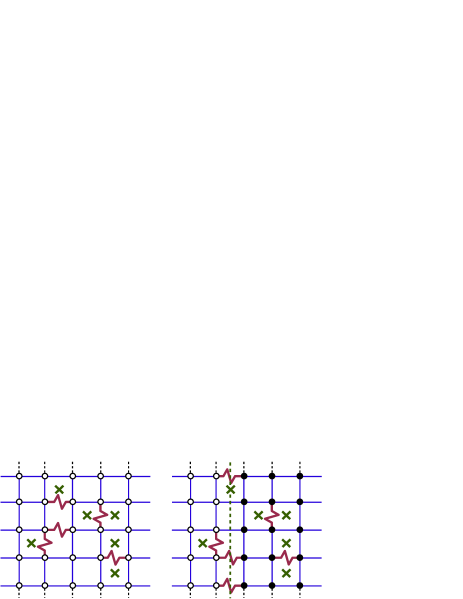
Figure 1: (Color online) An example of a $2J$ excitation. On the left is a ground state configuration with six frustrated plaquettes and five unsatisfied (jagged) bonds. On the right is a first excited state obtained by flipping all spins on one side of the vertical broken line. The excited state has six unsatisfied bonds. Periodic BCs are indicated by the top and bottom dashed vertical lines.

Our main message here is that it is possible to essentially define the ferromagnetic phase by the absence of these $2J$ excitations. Alternative approaches AH04 include the imposition of domain wall defects and the calculation of magnetisation. These nevertheless lack clear systematics due to the large degeneracy of the ground state. Domain wall defects may not represent excitations at all since they can correspond to alternative ground states. Sampling of domain walls cannot be done in a controlled way and it is not obvious MH07 how we can obtain typical representative domain walls.

Calculation of the magnetisation is also problematic as a result of the ground state degeneracy. In Ref. AH04, , for example, the algorithm starts with a ground state and proceeds with a Monte Carlo simulation to determine a typical value of the magnetisation.

In this work we propose a simple picture of the ferromagnetic phase that is evaluated from the response to temperature alone. The number of lowest energy excitations is counted exactly. In the thermodynamic limit these excitations can only exist in the spin glass phase. Details of our results are given in Sec. III after a brief account of our method.

II Formalism

We use the Pfaffian method and degenerate state perturbation theory to calculate the degeneracies of the excited states. The planar Ising model can be mapped onto a system of noninteracting fermions. Each bond is decorated with two fermions, one either side. A square plaquette then has four fermions inside and four others across the bonds, as shown in Fig. 2. For a system with $N$ lattice sites we have $4N$ fermions in total. The partition function can be written as GH64 ; B82

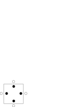
Figure 2: A plaquette with associated lattice fermions. The filled circles are associated with the plaquette, and the pairs of filled and open circles are associated with the bonds.

$$Z=2^{N}\left(\prod_{\langle ij\rangle}\cosh(J_{ij}/kT)\right)(\det D)^{1/2}.$$ (1)

The product is over all nearest-neighbor bonds $J_{ij}$ on an $N$ site lattice. The matrix $D$ is a $4N\times 4N$ skew-symmetric matrix that comprises constant diagonal blocks, and off-diagonal blocks that depend on temperature $T$ through matrix elements $\pm\tanh J_{ij}/kT$. The factor $(\det D)^{1/2}$ is precisely the Pfaffian GH64 ; B82 . This formalism is applicable to any distribution of disorder. For the bimodal model $J_{ij}=\pm J$.

At zero temperature there are defect eigenstates of $D$ with eigenvalues equal to zero. Each defect eigenstate can be expressed as a linear combination of the fermions localized in a frustrated plaquette. The number of these defect eigenstates is exactly equal to the number of frustrated plaquettes. At low temperature each defect eigenvalue approches zero as

$$\epsilon=\pm\frac{1}{2}X\exp\left(-\frac{2Jr}{kT}\right)$$ (2)

where $r$ is an integer and $X$ is a real number. These quantities $r$ and $X$ can be obtained using degenerate state perturbation theory BP91 . The ground state energy is written as

$$U_{0}=-2NJ+2J\sum_{d}r_{d}$$ (3)

where the sum are over all defect eigenstate pairs. The ground state degeneracy is

$$M_{0}=\prod_{d}X_{d}$$ (4)

and the ground state entropy can then be written as $S_{0}=k\sum_{d}\ln X_{d}$.

At arbitrary low temperature the internal energy can be expanded as Wanyok

$$U=U_{0}+\sum_{m=1}^{\infty}e^{-2Jm/kT}U_{m}$$ (5)

where the coefficient $U_{m}$ is expressed as

$$U_{m}=-2^{m}J\ \text{Tr}\ R^{m}$$ (6)

with

$$R=D_{1}g_{c1}(1+D_{1}G_{1})(1+D_{2}G_{2})\cdots(1+D_{r_{max}}G_{r_{max}}).$$ (7)

The $2\times 2$ block diagonal matrix $D_{1}$ is defined according to $D=D_{0}+\delta D_{1}$ where $D_{0}$ is the matrix $D$ when $T=0$ and $\delta=1-\tanh J/kT$. $D_{1}$ has non-zero matrix elements joining two fermions across bonds only. The $4\times 4$ block diagonal matrix $g_{c1}$ is derived from the continuum Green’s function BP91 and has matrix elements connecting the fermions within a plaquette. $D_{2}$ is given by $D_{2}=D_{1}g_{c1}D_{1}$ and, for $r>2$, $D_{r}=D_{r-1}(1+G_{r-2}D_{r-2})\cdots(1+G_{1}D_{1})g_{c1}D_{1}$. The Green’s function $G_{r}$ is given by BP91

$$G_{r}=-\sum_{i=1}^{N(r)}\lvert r,i\rangle\left(\frac{1}{\epsilon^{i}_{r}}\right)\langle r,i\rvert,$$ (8)

where $\lvert r,i\rangle$ is the ground state defect eigenstate of $D$ with eigenvalue $\epsilon^{i}_{r}$. The integer $r$ represents the order of perturbation theory at which the degeneracy is lifted. It is also the index $r$ in Eq. (2). The total number of such eigenstates is $N(r)$.

The coefficient $U_{m}$ can also be expressed in terms of the degeneracies of the excited states. We denote the degeneracy of the ith excited state as $M_{i}$. The partition function of the bimodal Ising model can be expressed in terms of the degeneracies as

$$Z=2M_{0}e^{-\frac{U_{0}}{kT}}\left(1+\frac{M_{1}}{M_{0}}e^{-\frac{2J}{kT}}+\frac{M_{2}}{M_{0}}e^{-\frac{4J}{kT}}+\ldots\right).$$ (9)

Using some thermodynamic relations together with the expansion of $\ln Z$ using the Taylor series $\ln(1+x)=x-\frac{x^{2}}{2}+\frac{x^{3}}{3}-\ldots$, we obtain, for example,

$$U_{1} = 2J\left(\frac{M_{1}}{M_{0}}\right)$$

$$U_{2} = 4J\left(\frac{M_{2}}{M_{0}}-\frac{1}{2}\left(\frac{M_{1}}{M_{0}}\right)^{2}\right)$$

$$U_{3} = 6J\left(\frac{M_{3}}{M_{0}}-\frac{M_{2}}{M_{0}}\frac{M_{1}}{M_{0}}+\frac{1}{3}\left(\frac{M_{1}}{M_{0}}\right)^{3}\right)$$ (10)

From these relations the ratios $\frac{M_{i}}{M_{0}}$ for all excited states can be obtained recursively. Note that $M_{1}$ is the number of $2J$ excitations.

III results

We have calculated $\frac{M_{1}}{M_{0}}$ for system sizes up to $L=129$ and concentrations $p$ ranging from 0.050 to 0.150. The number of disorder realizations ranges from 20000 for the smallest size to 2000 for the largest. We denote as $P_{1}$ the probability of finding $\frac{M_{1}}{M_{0}}>0$. In Fig. 3, $P_{1}$ is plotted as a function of system size $L$ for various defect concentrations. The error bars are evaluated using the bootstrap method E82 . The transition concentration $p_{c}$ is indicated where the $L$ dependency of $P_{1}$ changes from decreasing to increasing. We can see that $P_{1}$ is decreasing for $p<0.102$. The system can be regarded as ferromagnetic below this concentration. Since $P_{1}$ is increasing with $L$ for $p>0.106$, the system can be regarded as a spin glass. We conclude from these results that the value of $p_{c}$ lies between 0.102 and 0.106.

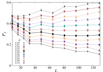
Figure 3: (Color online) The probability $P_{1}$ of finding $\frac{M_{1}}{M_{0}}>0$, plotted as a function of system size $L$ for various values of antiferromagnetic bond concentration $p$.

We have done a scaling plot using the relation KR97 ,

$$P_{1}L^{\psi}=f((p-p_{c})L^{\phi}).$$ (11)

It is reasonable to fix $\psi=0$ since the value of $P_{1}$ is bounded to the range [0,1]. In any case, with $\psi$ not fixed, the best scaling plots have $\psi<0.001$. The parameters $p_{c}$ and $\phi$ are chosen to minimize the quality parameter HH04 ; M09 $S$. The best fits give $p_{c}=0.1045(11)$ and $\phi=0.532(72)$ with $S=0.62$. The resulting scaling plot is shown in Fig. 4. The error bars of each parameter are obtained using the method described in Ref. AH04, . We fix the corresponding parameter at various values and minimize $S$ with respect to the other parameter. The range of the fixed parameter that gives $S$ double the minimum value is regarded as the error bar. For example we show in Fig. 5 the variation of the partial minimized value of $S(p_{c},\phi)$ as a function of $p_{c}$. The error bar of $\phi$ can be obtained in the same way.

The above value of $p_{c}$ agrees, within error bars, with $p_{c}=0.103(1)$ proposed in Ref. AH04, . Note that we also performed the analysis using data from systems with $L\leq 65$ and get $p_{c}\gtrsim 0.105$. This indicates that the effect of finite size is the overestimation of $p_{c}$. It is expected that if we perform this analysis using data with $L>129$, we will get a smaller value of $p_{c}$.

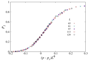
Figure 4: (Color online) The scaling plot of $P_{1}$ as a function of the antiferromagnetic bond concentration $p$ with $p_{c}=0.1045(11)$ and $\phi=0.532(72)$.

Figure 5: The variation of $S_{min}$ as a function of $p_{c}$.

We have also investigated the distributions of the $2J$ excitations in the ferromagnetic phase. We denote as $C_{1}(x)$ the probability of finding $\frac{M_{1}}{M_{0}}\leq x$. In Fig. 6, $C_{1}(x)$ with $p=0.090$ is plotted for various values of $L$. It is clear that the most likely value of $\frac{M_{1}}{M_{0}}$ is zero. The probability of getting $\frac{M_{1}}{M_{0}}>0$ is decreasing with $L$. We may expect that in the ferromagnetic phase the $2J$ excitations vanish in the thermodynamic limit.

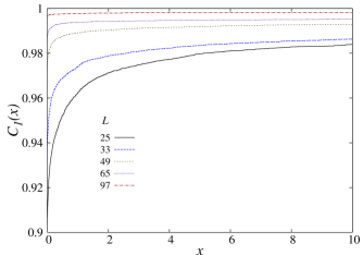
Figure 6: (Color online) The probability $C_{1}(x)$ of finding $\frac{M_{1}}{M_{0}}\leq x$ for $p=0.090$.

Since there are no $2J$ excitations in the ferromagnetic phase in the thermodynamic limit, the first excited state has energy $4J$. We have investigated the behavior of the $4J$ excitations by calculating the ratio $\frac{M_{2}}{M_{0}}$ for system sizes up to $L=97$. We denote as $H_{2}(x)$ the probability density function of getting $\frac{1}{L^{2}}\frac{M_{2}}{M_{0}}=x$. We use the kernel density estimation algorithm BGK10 to obtain $H_{2}(x)$. In Fig. 7, $H_{2}(x)$ with $p=0.090$ is plotted for various odd values of $L$. A sharp peak develops with increasing $L$. We expect to get a definite value of $\frac{1}{L^{2}}\frac{M_{2}}{M_{0}}$ in the thermodynamic limit. It is interesting that this behaviour does not depend on whether $L$ is odd or even. In Fig. 8, $H_{2}(x)$ with $p=0.090$ is plotted for various even values of $L$. The distributions are much the same and provide the same conclusions. From these results we have that the energy gap in the ferromagnetic phase is $4J$.

We can expect this also from the behavior of the specific heat at low temperature. When the temperature is low enough the behavior is dominated by the first excited state and can be expressed as KLC07

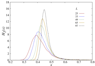
Figure 7: (Color online) The probability density $H_{2}(x)$ of getting $\frac{1}{L^{2}}\frac{M_{2}}{M_{0}}=x$ for $p=0.090$ with odd $L$.

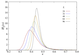
Figure 8: (Color online) The probability density $H_{2}(x)$ of getting $\frac{1}{L^{2}}\frac{M_{2}}{M_{0}}=x$ for $p=0.090$ with even $L$.

$$c_{v}=\frac{16J^{2}}{kT^{2}}\left(\frac{1}{L^{2}}\frac{M_{2}}{M_{0}}\right)e^{-4J/kT}.$$ (12)

Sharpness of the distribution of $\frac{1}{L^{2}}\frac{M_{2}}{M_{0}}$ satisfies the requirement of $c_{v}$ as a physical quantity. We can expect that in the ferromagnetic phase the specific heat has a definite value in the thermodynamic limit. At low temperature $c_{v}$ is proportional to $\exp(-4J/kT)$ and the energy gap can be regarded as $4J$.

The distribution of the $2J$ excitations in the spin glass phase is quite different. In Fig. 9, $C_{1}(x)$ with $p=0.110$ is plotted for various values of $L$. Although the most likely value of $\frac{M_{1}}{M_{0}}$ is still at zero, the probability of getting $\frac{M_{1}}{M_{0}}>0$ is increasing with $L$. The distributions of $\frac{M_{1}}{M_{0}}$ do not have a sharp peak but broaden when $L$ is increasing. We have that the $2J$ excitations persist as $L$ increases.

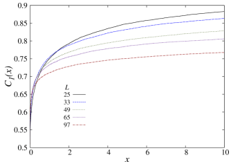
Figure 9: (Color online) The probability $C_{1}(x)$ of finding $\frac{M_{1}}{M_{0}}\leq x$ for $p=0.110$.

The distribution of the $4J$ excitations in the spin glass phase is also different from that in the ferromagnetic phase. In Fig. 10, $H_{2}(x)$ with $p=0.110$ is plotted for various odd values of $L$. The most likely value of $H_{2}(x)$ increases with $L$ and the distributions broaden. This behavior of $H_{2}(x)$ is similar Wanyok to that of the canonical spin glass ($p=0.5$) with even $L$. In particular, the height of the peak of the distribution collapses with increasing $L$. We have also checked the distributions of $H_{2}(x)$ with $p=0.110$ and even $L$. The results are shown in Fig. 11. The characteristics are the same for both odd and even $L$.

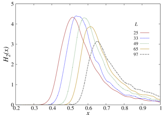
Figure 10: (Color online) The probability density $H_{2}(x)$ of getting $\frac{1}{L^{2}}\frac{M_{2}}{M_{0}}=x$ for $p=0.110$ with odd $L$.

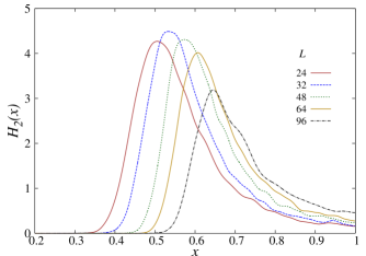
Figure 11: (Color online) The probability density $H_{2}(x)$ of getting $\frac{1}{L^{2}}\frac{M_{2}}{M_{0}}=x$ for $p=0.110$ with even $L$.

IV Summary

We have proposed a simple view that distinguishes between the ferromagnetic and spin glass phases. The ferromagnetic phase is characterised by the absence of lowest energy, that is $2J$ excitations. Our method counts the number of excitations exactly without bias. It is not necessary to work with some typical ground or excited state.

Distributions of the number of $2J$ excitations are shown to differ in character between the phases. In the ferromagnetic phase the number declines as the (odd) circumference $L$ of the cylindrical winding increases. A finite-size scaling analysis produces a data collapse of excellent quality to support our conclusion that $2J$ excitations do not exist in the thermodynamic limit of the ferromagnetic phase. In the spin glass phase the situation is reversed with the degeneracy of the first excited state increasing with $L$.

The energy gap in the ferromagnetic phase is $4J$. For even values of $L$ the first excitations have energy $4J$. We have also presented distributions of $4J$ excitations so as to indicate that there is no essential dependence on whether $L$ is even or odd. In the ferromagnetic phase the peak grows taller and narrower with increasing $L$ and will presumably lead to a unique value of the low temperature specific heat in the thermodynamic limit.

In the spin glass phase the behaviour of the distributions is quite different. Essentially they are extreme with long tails. As $L$ increases the tails become fatter and the peak collapses. We believe that this is consistent with a power law behaviour for the low temperature specific heat. The extreme distributions only indicate spin glass behaviour; a proper statistical mechanical description of the model requires a summation over the entire density of states. This seems to suggest that thermally active droplets can indeed take many different values of energy.

Finally, we have not found any evidence that indicates a random antiphase state BMR82 , although we cannot rule out a situation where percolation of rigid bonds coexists with zero magnetization.

- (1) K. Binder and A. P. Young, Rev. Mod. Phys. 58, 801 (1986).
- (2) M. Mézard, G. Parisi and M. Virasoro, Spin Glass Theory and Beyond (World Scientific, Singapore, 1987).
- (3) K. H. Fischer and J. A. Hertz, Spin Glasses (Cambridge University Press, Cambridge, 1991).
- (4) N. Kawashima and H. Rieger, Frustrated Spin Systems, edited by T. H. Diep (World Scientific, Singapore, 2004).
- (5) S. F. Edwards and P. W. Anderson, J .Phys. F: Met. Phys. 5, 965 (1975).
- (6) A. K. Hartmann and H. Rieger, Optimization Algorithms in Physics (Wiley-VCH, Berlin, 2002).
- (7) A. K. Hartmann, Practical Guide to Computer Simulations (World Scientific, Singapore, 2009).
- (8) G. Toulouse, Commun. Phys. 2, 115 (1977).
- (9) M. Ohzeki and H. Nishimori, J. Phys. A: Math. Theor. 42, 332001 (2009).
- (10) C. Wang, J. Harrington and J. Preskill, Ann. Phys. 303, 31 (2003).
- (11) C. Amoruso and A. K. Hartmann, Phys. Rev. B 70, 134425 (2004).
- (12) F. P. Toldin, A. Pelissetto and E. Vicari, J. Stat. Phys. 135, 1039 (2009).
- (13) J. A. Blackman, J. R. Gonçalves and J. Poulter, Phys. Rev. E 58, 1502 (1998).
- (14) J. Lukic, A. Galluccio, E. Marinari, O. C. Martin and G. Rinaldi, Phys. Rev. Lett. 92, 117202 (2004).
- (15) F. Barahona, R. Maynard, R. Rammal and J. P. Uhry, J. Phys. A: Math. Gen. 15, 673 (1982).
- (16) F. Romá, S. Risau-Gusman, A. J. Ramírez-Pastor, F. Nieto and E. E. Vogel, Phys. Rev. B 82, 214401 (2010).
- (17) W. L. McMillan, J. Phys. C 17, 3179 (1984).
- (18) A. Bovier and J. Fröhlich, J. Stat. Phys. 44, 347 (1986).
- (19) D. S. Fisher and D. A. Huse, Phys. Rev. Lett. 56, 1601 (1986).
- (20) A. J. Bray and M. A. Moore, Heidelberg Colloquium on Glassy Dynamics edited by J. L. van Hemmen and I. Morgenstern (Springer,Berlin, 1987), p.121.
- (21) D. S. Fisher and D. A. Huse, Phys. Rev. B 38, 386 (1988).
- (22) W. L. McMillan, Phys. Rev. B 29, 4026 (1984); 30, 476 (1984); 31, 340 (1985).
- (23) A. J. Bray and M. A. Moore, J. Phys. C 17, L463 (1984); Phys. Rev. B 31, 631 (1985); Phys. Rev. Lett. 58, 57 (1987).
- (24) A. K. Hartmann and A. P. Young, Phys. Rev. B 66, 094419 (2002).
- (25) N. Kawashima and H. Rieger, Europhys. Lett. 39, 85 (1997).
- (26) A. K. Hartmann, Phys. Rev. B 77, 144418 (2008).
- (27) P. Dayal, S. Trebst, S. Wessel, D. Würtz, M. Troyer, S. Sabhapandit and S. N. Coppersmith, Phys. Rev. Lett. 92, 097201 (2004).
- (28) W. Atisattapong and J. Poulter, New J. Phys. 10, 093012 (2008).
- (29) J.-S. Wang, Phys. Rev. E 72, 036706 (2005).
- (30) J.-S. Wang and R. H. Swendsen, Phys. Rev. B 38, 4840 (1988).
- (31) T. Jorg, J. Lukic, E. Marinari and O. C. Martin, Phys. Rev. Lett. 96, 237205 (2006).
- (32) C. K. Thomas, D. A. Huse and A. A. Middleton, Phys. Rev. Lett. 107, 047203 (2011).
- (33) H.-F. Cheung and W. L. McMillan, J. Phys. C 16, 7033 (1983).
- (34) J. Houdayer and A. K. Hartmann, Phys. Rev. B 70, 014418 (2004).
- (35) H. G. Katzgraber, L. W. Lee and I. A. Campbell, Phys. Rev. B 75, 014412 (2007).
- (36) L. Saul and M. Kardar, Phys. Rev. E 48, R3221 (1993); Nucl. Phys. B 432, 641 (1994).
- (37) J. Lukic, E. Marinari, O. C. Martin and S. Sabatini, J. Stat. Mech. (2006) L10001.
- (38) F. Romá, S. Risau-Gusman, A. J. Ramirez-Pastor, F. Nieto and E. E. Vogel, Phys. Rev. B 75, 020402 (2007).
- (39) O. Melchert and A. K. Hartmann, Phys. Rev. B 76, 174411 (2007).
- (40) M. Weigel and D. Johnston, Phys. Rev. B 76, 054408 (2007).
- (41) A. Aromsawa and J. Poulter, Phys. Rev. B 76, 064427 (2007).
- (42) J. A. Blackman and J. Poulter, Phys. Rev. B 44, 4374 (1991).
- (43) H. G. Katzgraber and L. W. Lee, Phys. Rev. B 71, 134404 (2005).
- (44) H. S. Green and C. A. Hurst, Order-Disorder Phenomena (Interscience, London, 1964).
- (45) J. A. Blackman, Phys. Rev. B 26, 4987 (1982).
- (46) B. Efron, The Jackknife, the Bootstrap and Other Resampling Plans (Society of Industrial and Applied Mathematics, Philadelphia, 1982).
- (47) O. Melchert, arXiv:0910.5403v1 (unpublished).
- (48) Z. I. Botev, J. F. Grotowski and D. P. Kroese, Ann. Statist. 38, 2916 (2010).