Generalized Eaton Lens at Arbitrary Refraction Angles

Abstract

We extended the refraction angle of the Eaton lens into arbitrary angles. The refractive index of the Eaton lens is not analytical and can be obtained by numerical calculations only except in the case of the retroreflector. We introduced an approximation for the refractive index of the generalized Eaton lens. It is simple but very close to the exact values obtained from numerical calculations.

Trajectories of light can be controlled by prisms or a combination of mirrors. At the same time it can be achieved by controlling the refractive index(RI) of a lens. It is a GRIN(Gradient Index) lens. Once it was thought to be unrealistic or very difficult to realize, but the recent development of transformation optics and high RI materials from metamaterial techniques have opened a new way to control the trajectories of waves.

The Eaton lens is a typical GRIN lens where the RI varies from one to infinity. It has a singularity at the center of the lens that the RI goes to infinity and it originates from a singularity of dielectrics. The speed of light reduces to zero at the singularity, therefore, the lens can change the trajectories of waves into any direction.

For the three specific refraction angles such as $90^{o}$(right-bender), $180^{o}$(retroreflector), and $360^{o}$(time-delayer), the Eaton lens has been studied recently hannay ; tomas ; danner . The RI of the Eaton lens is given as a function of radius, but it is not analytic except for the special refraction angle of the retroreflector. It is obtained by numerical calculations only. Then that makes the application of the lens to be inconvenient and is not easy to handle.

In this short note, the RI of Eaton lens is extended to arbitrary refraction angles. The generalized form of the RI is not analytic. To overcome the inconvenience, an approximated form of the RI is suggested for easy and practical use. It comes from a linear approximation of the retroreflector. Needless to say it should be very close to the numerical values at some realistic refraction angle ranges.

The RI for the three specific refraction angles have been studied already. For symmetric and spherical lenses they are known as danner

$$n^{2} = \frac{1}{nr}+\sqrt{\frac{1}{n^{2}r^{2}}-1}\hskip 10.0pt(\theta=90^{o}),$$ (1)

$$n = \sqrt{\frac{2}{r}-1}\hskip 52.0pt(\theta=180^{o}),$$ (2)

$$\sqrt{n} = \frac{1}{nr}+\sqrt{\frac{1}{n^{2}r^{2}}-1}\hskip 9.0pt(\theta=360^{o}).$$ (3)

$n=1$ for $r\geq 1$, where $n$ is the relative RI. The $r$ is the radial position between 0 and 1, and the actual radial position is given by $ar$, where $a$ is the radius of the lens.

The importance of the above three lenses has been discussed. The right-bender in Eq. (1) has been studied in a bending surface plasmon polaritons zent . The retroreflector in Eq. (2) is a device that returns the incident wave back to their source ma . The time-delayer in Eq. (3) is a time clocking device that the incident wave leaves in the direction of incidence as if the lens were not present. The trajectories for the above three cases has been plotted by Danner and Leonhardt danner . It is shown in Fig. 1.

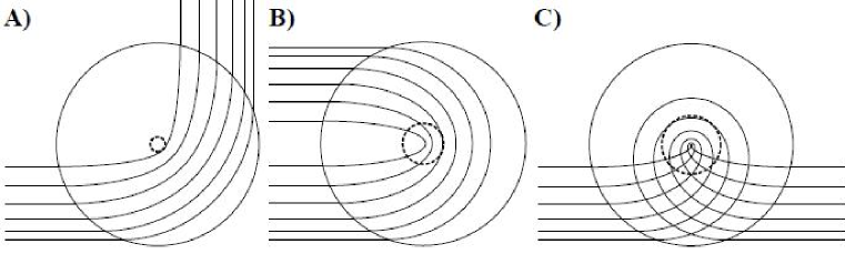
Figure 1: The trajectories of Eaton lenses at three specific angles from Ref. danner . (A)$90^{o}$, (B)$180^{o}$, (C)$360^{o}$.

The RI of arbitrary refraction angles is easily derived from Ref. hannay . RI is identical to particle trajectories of equal total energy $E$ in a central potential $U(r)$. From the conservation of mechanical energy inside and outside the lens, the kinetic energy of a particle in the medium of RI $n$ is written as $(1/2)mn^{2}v^{2}=E-U$, where $m$ is the mass and $v$ is the velocity of the particle inside the lens. Then, $\int nds$ or $\int\sqrt{E-U}ds$ should be stationary by Fermat’s principle. The potential of the Eaton lens corresponds to $U\propto-1/r$ hannay . On the other hand the potential Luneburg lens corresponds to $U\propto r^{2}$ morgan . The trajectory of the Eaton lens is an analogue of Kepler’ scattering problem landau .

Replacing $\chi+\pi=\theta_{final}-\theta_{initial}$ into $\theta$ in Ref. hannay , we obtain a generalized form of the RI of Eaton lens at arbitrary refraction angles as

$$\small n^{\pi/\theta}=\frac{1}{nr}+\sqrt{\frac{1}{n^{2}r^{2}}-1},$$ (4)

where $\theta$ is any radian angle and $n=1$ for $r\geq 1$. The refraction angle can be generalized as $\theta=(2N+1/2)\pi$ for right-bender, $\theta=(2N+1)\pi$ for retroreflector, and $\theta=2N\pi$ for time-delayer. Note that $N$ is an integer. The RI is not analytic still. We calculated numerically and plotted RI for four specific angles in Fig. 2

Figure 2: The refractive indexes at $\theta=90^{o},180^{o},270^{o}$, and $360^{o}$ from left to right.

Taking logarithm we have a more convenient form of the relations between RI and the radius.

$$\small\frac{\theta(n,r)}{\pi}=\frac{\log n}{\log\left(\frac{1}{nr}+\sqrt{\frac{1}{n^{2}r^{2}}-1}\right)}.$$ (5)

For any given radius and RI, we can predict the refraction angle from Eq. (5). It is plotted in Fig. 3. Large RI changes the trajectories at small radius. They are almost inversely proportional to each other.

Figure 3: The refraction angles at various refractive index and radius.

Figure 4: $p(r)$ as a function of radius. $\theta=90^{o},180^{o},270^{o}$, and $360^{o}$ from top to bottom. $p(r)$ is linear for $\theta=180^{o}$

Eq. (5) is relatively convenient to find the relations between RI and radius than Eq. 4, but still not practical. We need an analytic form in lab to apply.

From Eq. (4) we obtain $n(r)$ at two boundaries. As $r\sim 0$, then $n\sim(2/r)^{\theta/(\pi+\theta)}$. And as $r\sim 1$, then $n\sim(1/r)^{\theta/(\pi+\theta)}$. Therefore, we can write $n(r)$ at the range of $0<r\leq 1$ as the following compact form

$$n(r)=\left\{\frac{p(r)}{r}\right\}^{\frac{\theta}{\pi+\theta}},$$ (6)

where $0<p(r)\leq 1$.

The $p(r)$ is a bounded and analytic function of radius between 1 and 2. It is obtained from

$$\small p(r)=rn(r)^{\frac{\pi+\theta}{\theta}}.$$ (7)

$p(r)$ is plotted in Fig. 4. It is monotonically decreasing from $r=0$ to $r=1$. It is pretty linear. Therefore, we can take the retroreflector approximation or a linear approximation as $p(r)=2-r$. Then, the RI has a simple form as

$$\small n(r)\simeq\left(\frac{2}{r}-1\right)^{\frac{\theta}{\pi+\theta}}.$$ (8)

Figure 5: Comparison between the exact value obtained by numerical calcultion and the retroreflector approximation for $\theta=90^{o},270^{o}$. They are match exactly for $\theta=180^{o}$. They matches at both ends of $r\sim 0$ and $r\sim 1$ at every angles.

The effectiveness of the approximation is examined by comparison with some exact values obtained from numerical calculation in Fig. 5. We see the approximation is pretty good at the range of $0<\theta<2\pi$.

The time-delayer with $\theta=2N\pi$ is an invisible sphere. The general form with $N$ turn can be represented easily using $p(r)$ in Eq. (6). When it has $N$ turn, the time delay $\triangle t$ is obtained as

$$\small\triangle t=\frac{2N\pi rn}{v_{o}}=\frac{2N\pi r}{v_{o}}\left\{\frac{ap(r)}{r}\right\}^{\frac{2N}{2N+1}},$$ (9)

where $v_{o}$ is the background velocity outside the lens and $a$ is the radius of the lens. If $N\gg 1$, then $2N\pi a/v_{o}\leq\triangle t\leq 4N\pi a/v_{o}$. Therefore, $a$ and $N$ are the two main factors that decide the time delay.

The Eaton lens is a typical GRIN lens with a complicated RI which has been studied at some specific angles. We derived the RI of Eaton lens at arbitrary refractive angles. It is not analytical at most angles and inconvenient to find the values easily. We introduced a retroreflector approximation for the RI. It is simple but very close to the exact values of the RI that are obtained from numerical calculation.

We would like to thank C. K. Kim and S. H. Lee for useful discussions. This research was supported by Basic Science Research Program through the National Research Foundation of Korea(NRF) funded by the Ministry of Education, Science and Technology(2011-0009119)

References

- (1) J. H. Hannay and T. M. Haeusser, J. Mod. Opt. 40, 1437 (1993).
- (2) T. Tyc and U. Leonhardt, N. J. Phys. 10, 115038 (2008).
- (3) A. J. Danner and U. Leonhardt, 2009 Conference on Lasers and Electro-Optics(CLEO), Baltimore, MD, U. S. A. (2009).
- (4) L. D. Landau and E. M. Lifshitz, Mechanics, 3rd ed. Sec. 18 (Pergamon, Oxford, 1976).
- (5) T. Zentgraf, Y. Liu, M. H. Mikkelson, J. Valentine, and X. Zhang, Nature, Nano, 6, 151 (2011).
- (6) Y. G. Ma, C. K. Ong, T. Tyc, and U. Leonhardt, Nature, Mat. 8, 639 (2009).
- (7) S. P. Morgan, J. Appl. Phys. 29, 1358 (1958).