Searches for Metal-Poor Stars from the Hamburg/ESO Survey using the CH G-band

Abstract

We describe a new method to search for metal-poor candidates from the Hamburg/ESO objective-prism survey (HES) based on identifying stars with apparently strong CH G-band strengths for their colors. The hypothesis we exploit is that large over-abundances of carbon are common among metal-poor stars, as has been found by numerous studies over the past two decades. The selection was made by considering two line indices in the 4300  Å region, applied directly to the low-resolution prism spectra. This work also extends a previously published method by adding bright sources to the sample. The spectra of these stars suffer from saturation effects, compromising the index calculations and leading to an undersampling of the brighter candidates. A simple numerical procedure, based on available photometry, was developed to correct the line indices and overcome this limitation. Visual inspection and classification of the spectra from the HES plates yielded a list of 5,288 new metal-poor (and by selection, carbon-rich) candidates, which are presently being used as targets for medium-resolution spectroscopic follow-up. Estimates of the stellar atmospheric parameters, as well as carbon abundances, are now available for 117 of the first candidates, based on follow-up medium-resolution spectra obtained with the SOAR 4.1m and Gemini 8m telescopes. We demonstrate that our new method improves the metal-poor star fractions found by our pilot study by up to a factor of three in the same magnitude range, as compared with our pilot study based on only one CH G-band index. Our selection scheme obtained roughly a 40% success rate for identification of stars with [Fe/H] $<-1.0$; the primary contaminant is late-type stars with near solar abundances and, often, emission line cores that filled in the Ca ii K line on the prism spectrum. Because the selection is based on carbon, we greatly increase the numbers of known CEMP stars from the HES with intermediate metallicities $-2.0<$ [Fe/H] $<-1.0$, which previous survey efforts undersampled. There are eight newly discovered stars with [Fe/H] $<-3.0$ in our sample, including two with [Fe/H] $<-3.5$.

1. Introduction

The interest in stars with metallicities lower than about ten times the solar value ([Fe/H]$<$$-$1.0) has greatly intensified in the past few decades, due to their utility as probes of the chemical history and kinematics of the stellar populations of the Galaxy and the nucleosynthesis pathways explored by the first generations of stars. Among the most interesting stars for such applications are those with the lowest possible metallicity. These chemically most primitive stars are expected to provide one of the best windows on chemical evolution during the first 0.5-1 Gyr following the Big Bang. Such stars are extraordinarily rare (only four stars with [Fe/H]$<-4.5$ are known at present), and require inspection of very large samples of candidates to identify them. The key is being able to distinguish likely metal-poor stars from among the overwhelmingly greater numbers of solar or near-solar abundance stars in the Galaxy.

Beginning roughly 40 years ago with the pioneering work of Bond (1970, 1980), Slettebak & Brundage (1971), and Bidelman & MacConnell (1973), photographic objective-prism techniques were shown to be efficient sieves for the identification of large numbers of metal-poor (and chemically peculiar) stars for further study. These efforts were expanded by the HK Survey of Beers, Preston, & Shectman (Beers et al., 1985, 1992), and later by the Hamburg/ESO Survey (HES; Reimers & Wisotzki, 1997; Christlieb, 2003), to include fainter stars that explore farther into the halo system of the Galaxy where the largest numbers of metal-poor stars have been found. Both of these surveys sought to identify metal-poor candidates by visual (HK Survey) or digitized (HES) scans of the prism plates, looking for stars with weak or absent lines of Ca  ii in low-resolution spectra. Star-by-star follow-up medium-resolution spectroscopy for over 15,000 candidates from these two surveys consumed large amounts of 1.5m to 4m telescope time over the past two decades, but yielded over 3000 very metal-poor (VMP; [Fe/H] $<-2.0$) stars, and several hundred extremely metal-poor (EMP; [Fe/H] $<-3.0$) stars. See Beers & Christlieb (2005) for a more complete history of these efforts.

More recently, the Sloan Digital Sky Survey (SDSS; York et al., 2000), in particular the sub-surveys known as the Sloan Extension for Galactic Understanding and Exploration (SEGUE; Yanny et al., 2009) and SEGUE-2 (Rockosi et al., 2011) were able to obtain medium-resolution spectroscopy for almost 500,000 stars, including numerous metal-poor candidates selected on the basis of their broadband $ugriz$ colors. These efforts have yielded the identification of over 25,000 VMP stars and on the order of 1000 EMP stars. Even larger samples are expected to come from the Chinese LAMOST (Large sky Area Multi-Object fiber Spectroscopic Telescope; Zhao et al., 2006) and the Australian SkyMapper (Keller et al., 2007) projects.

One of the limitations of the metal-poor stars identified by the SDSS is that the sample has a bright limit of $g\sim 14.0$, set by the saturation level of the photometric scans used to identify candidates in the first place. To the extent that SDSS imaging is used for targeting LAMOST targets, this limit will similarly apply to that survey. Stars brighter than 14th magnitude require far less 6.5m-10m telescope time in order to obtain the high-resolution spectroscopy that enables detailed understanding of their abundance patterns, and hence are greatly desired. The SkyMapper project will not suffer this limitation, since it includes very short exposure times in its planned cadence. However, as we show below, it is possible to use the already available HES prism spectra and 2MASS (Two Micron All Sky Survey; Skrutskie et al., 2006) near-IR photometry to improve our ability to identify metal-poor candidates that include brighter stars.

Our technique is based on the observational fact that, at very low metallicity, an increasing fraction of very metal-poor stars exhibit strong over-abudances of carbon. The great majority of stars more metal-rich than [Fe/H] $=-1.0$ exhibit carbon-to-iron ratios, [C/Fe], that track closely with [Fe/H]. However, below [Fe/H] $=-2.0$, on the order of 20% of stars have [C/Fe]$>+1.0$ (Lucatello et al., 2006). The fraction of so-called carbon-enhanced metal-poor (CEMP, Beers & Christlieb, 2005) stars in the HK survey and the HES rises to 30$\%$ for [Fe/H] $<-$3.0, 40$\%$ for [Fe/H] $<-$3.5, and 75$\%$ for [Fe/H] $<-$4.0 (accounting for the recently discovered non-carbon-enhanced star with [Fe/H]$\sim-5.0$, identified by Caffau et al., 2011, from among metal-poor stars in the SDSS).

Carollo et al. (2011) have argued that the increase in the frequency of CEMP stars with declining metallicity is due to the fact that the outer-halo component of the Galaxy possesses about twice the fraction of CEMP stars relative to carbon-normal stars at a given low metallicity than the inner-halo component. The observed correlation between metallicity and CEMP fraction is a manifestation of the lower metallicity of outer-halo stars, which begin to dominate halo samples at low abundance. This idea can also account for the observed increase in the fraction of CEMP stars at a given metallicity as a function of height above the Galactic plane (Frebel et al., 2006; Carollo et al., 2011), and may have influenced previous reports of less than a 20% fraction of CEMP stars in the HES at very low metallicity (Cohen et al., 2005; Frebel et al., 2006, 2009).

The Aoki et al. (2007) study of some 26 CEMP stars reveals stars with [Fe/H] $<-$2.2 that do not exhibit evidence for the operation of the s-process (the CEMP-no stars). Furthermore, in two of the most iron-deficient stars known today, HE 0557-4840 ([Fe/H]= $-$4.8; Norris et al., 2007), and HE 0107-5240 ([Fe/H]= $-$5.3; Christlieb et al., 2002) no neutron-capture elements have been detected; in HE 1327-2326 ([Fe/H]= $-$5.4; Frebel et al., 2005), Sr has been detected, but the upper limit for Ba indicates that the Sr in this star was not produced in the main s-process. Besides that, three of the four known ultra metal-poor (UMP) and hyper metal-poor (HMP) stars have huge over-abundances of CNO, up to several thousand times the solar ratios. Thus, it seems evident that the mechanisms by which carbon (and similarly N and O) has been enhanced in metal-deficient stars are likely to be much more diverse than can be accounted for by any single process. Corroborating this hypothesis, Cooke et al. (2011) reports on the identification of a high redshift, extremely metal-poor ([Fe/H]$\sim-$3.0) Damped Lyman Alpha (DLA) system with an observed pattern of CNO that closely resembles that of the UMP stars.

These results immediately suggest that at some early time in the Universe a significant amount of carbon was produced, by one or more of the following sources: (1) a primordial mechanism from massive, zero-metallicity, rapidly rotating stellar progenitors (Hirschi et al., 2006; Meynet et al., 2006, 2010), (2) production by “faint supernovae”, which eject large amounts of CNO during their explosions (Umeda & Nomoto, 2005; Kobayashi et al., 2011), or (3) production of carbon by stars of intermediate mass, which can be prodigious manufacturers of carbon during their AGB stages, followed by mass transfer to a surviving lower-mass companion. It remains possible that all three sources have played a role.

Placco et al. (2010) (hereafter Paper I) shows that it is possible to search for metal-poor stars based on the premise that a large fraction of them will also be carbon enhanced, and that fraction will increase at the lowest metallicities. They reported that, by making a selection based on a new line index for the CH G-band (GPE – applied to the low-resolution HES prism spectra) as a function of 2MASS $(J-K)_{0}$ color, more than 65% of their candidates had [Fe/H] $<-1.0$, while some 23% had [Fe/H] $<-2.0$, based on medium-resolution spectroscopic follow-up. Not surprisingly, many of the candidates turned out to be CEMP stars as well. The technique clearly works, and what remains to be done is to refine this approach and improve its selection efficiency by eliminating sources of uninteresting candidates entering the sample.

The present study aims to extend the work initiated in Paper I by introducing an auxiliary line index for the CH G-band, one that we show below improves the fractions of bona-fide CEMP stars selected for follow-up spectroscopy by roughly a factor of two compared to our initial effort. In addition, we have increased our magnitude limit for medium-resolution observations and included the brighter stars from the HES, developing a correction scheme to reduce saturation effects on the line indices. By refining our methods to search for carbon-enhanced stars, we expect to continue increasing the number of known CEMP stars with intermediate metallicities, as well as explore regimes with [Fe/H] $<-3.0$, where carbon plays a major role in describing the chemical evolution processes and formation scenarios of our Galaxy.

This paper is outlined as follows. Section 2 introduces a new line index for the CH G-band. The main features of the HES database, as well as the criteria for extracting the second subsample and the development of saturation corrections for bright sources are presented in Section 3. Section 4 discusses the selection criteria applied to the HES database. The medium-resolution spectroscopic follow-up observations and estimates of atmospheric parameters and carbon abundances are described in Section 5. Finally, our conclusions and perspectives for future observational follow-up and further applications of the method are presented in Section 6.

2. EGP – Additional Line Index for Carbon

One of the motivations for developing an additional line index for the CH G-band is to increase the efficiency of the search for CEMP stars, and the very metal-poor stars they are often associated with. The GPE index from Paper I has proven to be effective in searching for CEMP stars, but when used alone it is subject to contamination from stars with spectra that have strong H$\gamma$ lines (since this feature is included in the band covered by the GPE index) and from overlaps and plate artifacts on HES plates.

Here we introduce a new line index for the CH G-band, as an alternative means of measuring the contribution of this feature to the removal of flux in this region, but without any dependence on continuum determination. This index is calculated in a similar fashion to the definition proposed by Smith & Norris (1983) and modified by Morrison et al. (2003). The 200 Å wide line band was chosen following the same arguments found in Paper I for the GPE index, which measures the contrast between the G-band and a fitted continuum in the same wavelength interval (see definition in Eqn. 1 of Paper I). The new EGP index consists of a flux ratio, integrated in intervals defined for both the line band and the red sideband, defined as:

$${\rm EGP}=-2.5~{}{\rm log}\left[\frac{\int_{4200}^{4400}I_{\lambda_{n}}~{}d\lambda}{\int_{4425}^{4520}I_{\lambda_{m}}~{}d\lambda}\right]$$ (1)

where $I_{\lambda_{n}}$ and $I_{\lambda_{m}}$ are the measured flux (in counts) for the line band and red sideband, respectively, and $d\lambda$ refers to the spectral resolution, in Å. The definition from Morrison et al. (2003) uses sidebands on both the red and blue sides of the line band. Due to the presence, for cool stars ($T_{\rm eff}$  $\lesssim$ 4500 K), of CN bands on the blue side of the line band (3883 Å and 4216 Å), the estimates for the integrated flux can be strongly affected by these features, which could compromise the index. Therefore, only the flux on the line band (200 Å wide; 4200-4400 Å) and the red sideband (4425-4520 Å) are used.

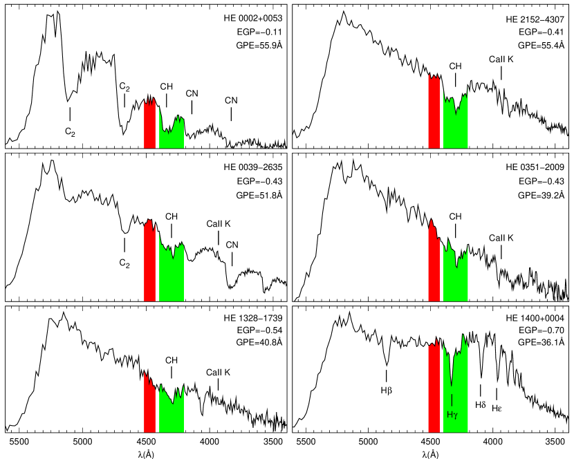
Figure 1.— Definition of the EGP index. The areas in red and green represent the sideband and the line band, respectively, for HES prism spectra of stars over a range of temperature and carbon enhancement. Note that the abscissa runs from red to blue wavelengths.

Figure 1 shows the wavelength intervals of the EGP index for the prism spectra of six stars from the HES plates. It is important to recall that, in contrast to the GPE index, EGP depends essentially on the depth of the G-band and the flux difference when compared to the contiguous red region of the spectra. It also possesses a smaller dynamical range (due to the logarithmic ratio) when compared to the GPE index. Nevertheless, this does not present the same difficulties exhibited by the formerly employed GP and GPHES indices (definitions in Beers et al., 1999; Christlieb et al., 2008, respectively), since the EGP does not use continuum estimates based on sideband linear interpolations.

From inspection of the center and bottom panels on the right side of Figure 1, one can see the advantage of introducing an auxiliary line index for the selection of CEMP stars. While the two objects present GPE values that differ by no more than 10%, the EGP difference reaches almost 50%. In those cases, the combination of the indices can be used as a filter for stars with prominent H$\gamma$ lines. Furthermore, this set of indices can be used to exclude spurious values of GPE, caused by (among others) overlapping spectra. Since both GPE and EGP measure the same region using different definitions, one should expect a reasonably strong correlation between the index values calculated for a given star. So, any large deviations from this expected behaviour can be interpreted as arising from possible contamination (see Section 4.2 for more details). Figure 2 shows how this effect can compromise the continuum calculation, and therefore the GPE value. One can see that the automated procedure fits the entire spectrum, and introduces a contamination on the index (see expanded detail in Figure 2). Thus, with the help of the EGP value, which is less affected by the overlap, one can exclude this type of object before going through the final visual inspection.

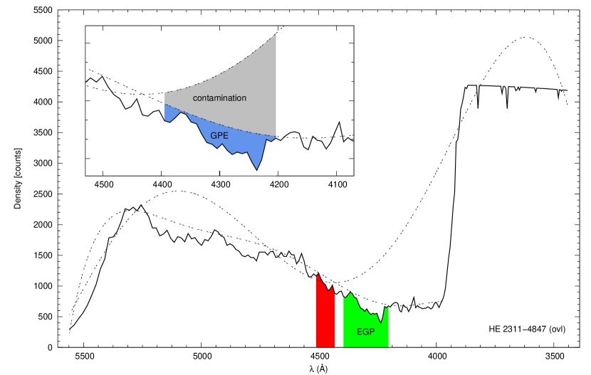
Figure 2.— Example of the ovl class from the HES, showing the definition of the EGP index. The dashed lines represent the continuum calculated for the whole spectra and the continuum estimated without the overlap. The expanded detail box shows a representation of the contamination of the GPE index by the overlapping spectra.

3. The HES Stellar Database

Even though it was originally designed to detect bright (V $<$ 16.5) quasars suitable for high-resolution spectroscopy, which drove the resolution requirement up to the point it was also useful for stellar science (Reimers, 1990; Wisotzki et al., 2000), the stellar data from the HES has been the subject of a great number of studies over the past decade (Christlieb et al., 2001, 2005; Barklem et al., 2005; Frebel et al., 2006; Aoki et al., 2007; Christlieb et al., 2008; Schörck et al., 2009; Li et al., 2010; Placco et al., 2010; Kennedy et al., 2011, and others), and has provided candidates for photometric follow-up, as well as moderate- and high-resolution spectroscopy.

The HES database presents a homogeneous, statistically well-understood sample of stars which can be used to assess many interesting questions regarding the origins of stellar populations and the formation of the Galaxy (see Beers & Christlieb, 2005). Both the spectral resolution (15 Å at Ca ii K – 3933 Å) and wavelength coverage (3200-5300 Å) of the HES spectra are suitable for searching for metal-poor stars by taking advantage of what has been learned about the behavior of the CH G-band (4300  Å) and Ca ii K line at low metallicity.

3.1. The Second HES Subsample

The present study made use of two classes of objects extracted from the HES objective-prism plates: stars and bright. The stars are point-like sources showing no signs of saturation in their spectra and the bright sources are objects close to (and above) the saturation threshold of the HES plates. For each of these types, a different set of restrictions was developed, including a more relaxed version of the method described in Christlieb et al. (2008), and applied to the database in order to reduce the number of spurious candidates for subsequent analysis.

3.1.1 Source Type: Stars

The selection criteria for the stars do not follow the same prescriptions found in Paper I, in hopes of removing any known sample-related biases, specially regarding the photometric quality and apparent magnitudes of the objects. The restriction on source type removes bright and extended sources from the HES. These extended sources can contaminate the selected sample with galaxy candidates, and the bright sources have a distinct selection criteria, described later in this section.

The (B$-$V)₀ colors were retrieved from the HES database, using the improved calibration described in Christlieb et al. (2008). A selection was then made in the color range 0.30 $\leq$(B$-$V)₀$\leq$ 1.00, in order to avoid stars outside the optimal color range for the atmospheric parameters calculation (see Section 5.2).

The J and K magnitudes were taken from the 2MASS All-Sky Data Release (Two Micron All Sky Survey; Skrutskie et al., 2006), and were used only for the objects labeled with the photometric quality flags “A”, “B” or “C”. The de-reddened (J$-$K)₀ colors were calculated based on the Schlegel et al. (1998) prescription. The selected objects lie in the color range 0.20 $\leq$(J$-$K)₀$\leq$ 0.75. Finally, restrictions were placed on the average signal-to-noise ratio in the calcium line region (SN${}_{\rm CaHK}>$ 5), as well as on the KP index, which was chosen to be greater than $-1.0\cdot\sigma_{\mathrm{KP}}$, where $\sigma_{\mathrm{KP}}$ is the detection limit for the Ca ii K line (see Figure 6 of Christlieb et al., 2008). The latter criterion aims at rejecting spectra that exhibit a Ca ii K line in emission, and for which negative KP indices are measured.

The HES stars fulfilling all of the above restrictions and contained inside both color intervals were then passed through the selection procedure in the KP/(B$-$V)₀ and KP/(J$-$K)₀ planes described in detail by Christlieb et al. (2008). However, the selection adopted in this work sets a more relaxed criterion for the metallicity cut, setting it at [Fe/H] =$-$2.0, rather than the more conservative limit of [Fe/H] =$-$2.5 employed by Christlieb et al. (2008). The objects selected were required to be found within the cut regions for at least one of the KP/color planes in order to be recognized as a metal-poor candidate. The final subset of the source type stars contains 62,311 candidates.

3.1.2 Source Type: Bright

The criteria for selecting bright sources is very similar to the one applied to the stars. The only difference is the exclusion of the KP/(B$-$V)₀ restriction, due to the fact that saturation effects play a major role on the accuracy of color determinations for the brightest stars from the HES (Frebel et al., 2006). Furthermore, since the absolute number of bright sources in the HES is on the order of 1/6th the number of stars, there was no need to introduce additional criteria to filter down the number of bright objects for visual inspection. The final subset of the source type bright contains 18,532 candidates.

One of the main goals of the present analysis is to apply a single set of contraints for both stars sources and for bright . However, as mentioned by previous studies (e.g. Frebel et al., 2006), the bright objects from the HES suffer saturation effects, which have to be dealt with before proceding with the analysis of the entire candidate list.

3.2. Saturation Corrections for Bright Sources

Saturation can effect most astronomical data, at least when photons are collected by material (photographic plates or CCDs) with a finite capacity for measuring light. For photographic plates the problem is actually more severe, due to non-linearities that begin to develop in the response curves even before the saturation level is reached. Hence, line indices that rely on comparisons of the relative densities of regions of spectrum on photographic plates will vary somewhat, even when stars of the same intrinsic compositions, temperatures, and surface gravities, but differing apparent magnitudes, are measured.

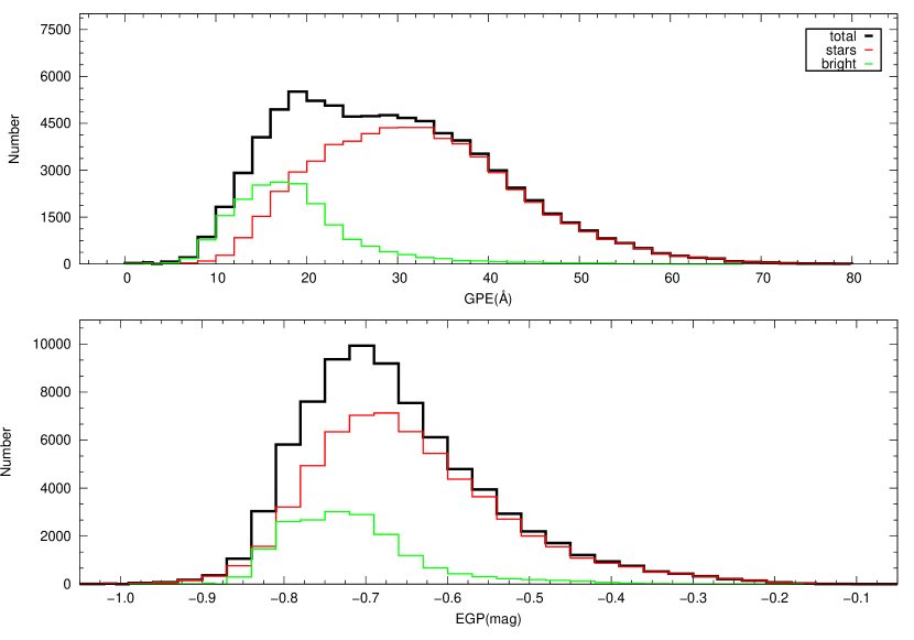
Figure 3.— Distribution of the CH G-band line indices for the second HES subsample, divided by source type as shown in the legend.

Figure 3 shows the distribution of the line indices for the 80,843 objects of the second HES subsample, divided by source type. It is clear that both GPE and EGP, as calculated for the candidates, do not share the same behaviour for the bright sources as seen for the stars. One might suppose mistakenly that the bright sources have intrinsically less carbon than the stars, which seems very unlikely. Rather, the histograms are misleading because the bright sources suffer much more than the stars from the saturation effects mentioned above, which have compromised their index calculations.

To compensate for this saturation issue for the bright sources, a numerical correction was developed, taking into account not only individual effects, but also trends for groups of objects. This correction was made by means of the spcmag variable from the HES, which is an internal magnitude based on the integrated photographic density in the B_J band. Determination of the particular value of B_J at which saturation occurs will vary, depending on the sensitivity of the individual HES plate, seeing conditions under which it was taken, and many other factors. As a result, this magnitude cannot be used to set the corrections for the line indices. However, spcmag is a good global indicator for the level of saturation; i.e., this indicator should be valid for all plates, since it measures the photographic density associated with the stars on each plate.

The distributions of B_J magnitude and spcmag, for both saturated and non-saturated sources, are shown in Figure 4. As can be appreciated from inspection, the two source types do not even share the same range of values. While the stars present a similar distribution as previous searches for metal-poor candidates (see Figure 10 of Christlieb et al., 2008), the bright sources appear in the same magnitude interval (9 $<{\rm B_{J}}<$ 14) as the bright objects studied by Frebel et al. (2006). Thus, the hypothesis is put forward that, for a given interval of spcmag, the bright sources will present the same saturation level for the line indices. That is, by looking at the index distribution of each spcmag interval of saturated and non-saturated sources, it is possible to estimate the amount of this saturation that translates into the index values. Then, to correct this effect, one should shift the distribution of line indices for each interval and match the distribution of the non-saturated sources.

Figure 4.— Distribution of B_J (BHES) and spcmag for the second HES subsample, divided by source type as shown in the legend.

The sample containing the bright sources (18,532 objects) was divided into nine parts according to the spcmag values. The normalized distributions for each part were compared with the normalized distribution of the non-saturated sources (containing all the 62,311 objects classified as stars). Figures 5 and 6 show, respectively, the distributions of the GPE and EGP indices for the individual parts. The black histograms represent the distribution for the non-saturated sources, and the ones in green are the index distributions for each of the nine divisions in spcmag. The histograms in red represent the corrected distributions. For each individual distribution, GPE_I, EGP_I, GPE_F and EGP_F are, respectively, the maximum values of the saturated (I) and non-saturated (F) distributions of the GPE and EGP indices. Thus, the saturation corrections for each division in spcmag are quantified by the required horizontal shift of each distribution, so that the saturated and non-saturated distributions match.

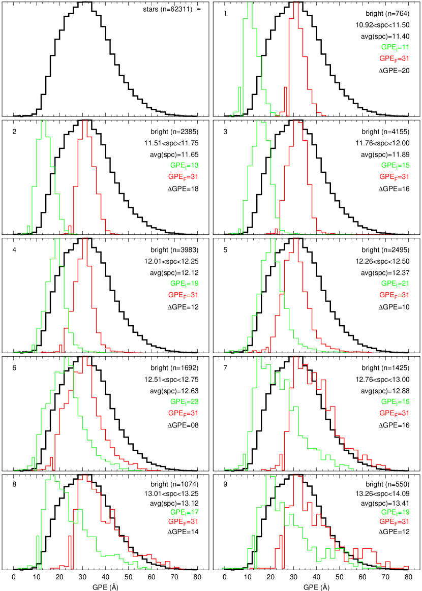
Figure 5.— Saturation corrections for GPE, shown over the range of spcmag. The black histograms represent the distribution for the non-saturated sources, and the ones in green are the index distributions in spcmag. The number of objects, magnitude range, and average values are shown on the upper right of the panels. The histograms in red represent the corrected distributions. GPE_I, EGP_I, GPE_F, and EGP_F are, respectively, the maximum values of the saturated (I) and non-saturated (F) distributions of the GPE and EGP indices. Thus, the saturation corrections for each division in spcmag are quantified by the horizontal shift of each distribution, listed in each panel as $\Delta$GPE, required to make the saturated and non-saturated distributions match.

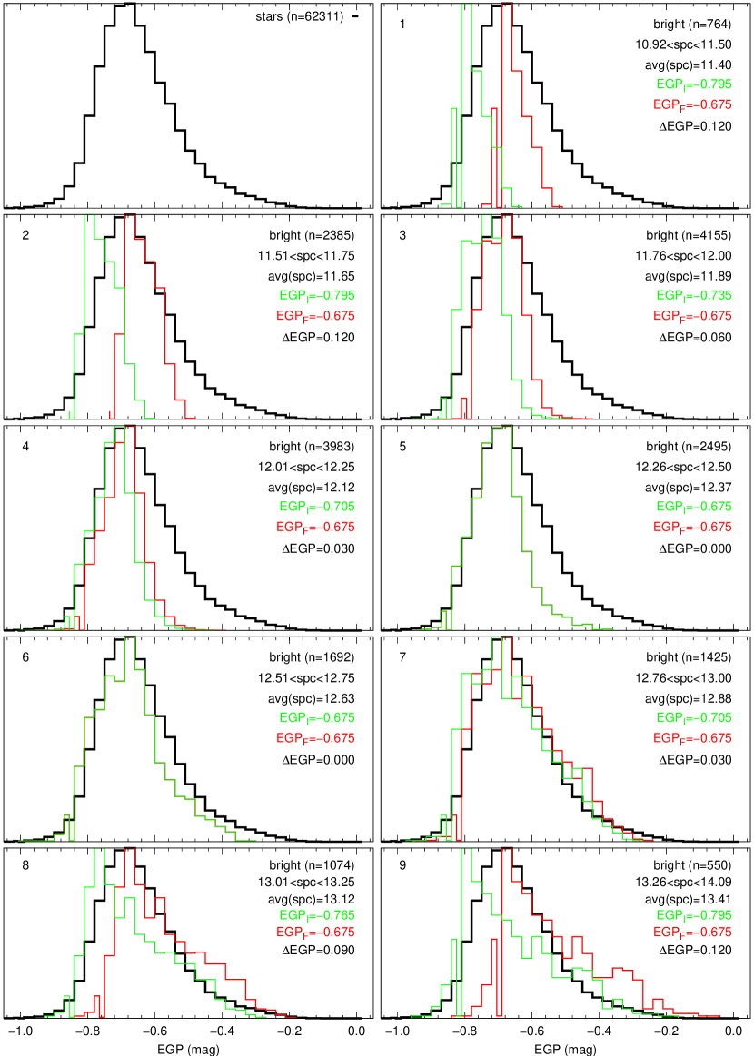
Figure 6.— Saturation corrections for EGP, shown over the range of spcmag. The approach is identical to that described for Figure 5, but for the EGP index.

It is interesting to note that the shifts in the EGP distributions are systematically smaller than the ones for the GPE, and can be as low as zero for 12.26 $<spcmag({\rm mag})<$ 12.70. This can be understood due to the differences in the calculations of the line indices, because the saturation has a greater effect on the continuum calculations than on the flux ratio. Besides that, the shifts tend to decrease with increasing spcmag, up to $\sim$12.75 mag, when the values start to increase. From inspection of Figures 5 and 6, one can conclude that this sudden increase (for spcmag$>$ 12.75 mag) is mainly because of the shape of the distributions. Given that those distributions contain fainter objects, associated with lower signal-to-noise spectra, the calculated index values are affected by the quality of the spectra and become more scattered. Hence, we chose to set aside the shifts determined for the last three distributions of Figures 5 and 6. For those (panels 7, 8 and 9), the shifts used were the ones associated with the distribution shown in panel 6.

Once determined, the shifts associated with each distribution of spcmag can be used to calculate the correction functions for GPE and EGP, by making polynomial fits to the [ avg(spc) , $\Delta$GPE ] and [ avg(spc) ,  $\Delta$EGP ] data pairs, as shown in Figure 7. There were a number of attempts to fit polynomials of degree 1-5 to the data available , and the lower values of the asymptotic standard errors for the final set of parameters are associated with a 4th degree polynomial (${\rm F_{GPE}}$ and ${\rm F_{EGP}}$). However, even this fit is not good for spcmag $<$ 11.40, where there is a sudden decrease of the data, and spcmag $>$ 12.63, that shows an unexpected increase of the shift values. Therefore, the corrections applied to the objects with spcmag $<$ 11.40 are those associated with the smaller values of avg(spc): 20 Å for GPE and 0.12 mag for EGP. For the objects with spcmag $>$ 12.63, 8Å is used for GPE and for EGP there are no corrections made. The final saturation correction criteria for the GPE and EGP indices are:

Figure 7.— Proposed correction function for the line indices, as a function of the average value of spcmag for each part of the distribution. Note that the last three points in each panel are not used (see text for explanation).

$$\Delta{\rm GPE(\AA)}=\left\{\begin{array}[]{rr}20.0,&spcmag<11.40\\ {\rm F_{GPE}},&11.40\leq spcmag\leq 12.63\\ 8.0,&spcmag>12.63\end{array}\right.\vspace{0.3cm}$$

$$\Delta{\rm EGP(mag)}=\left\{\begin{array}[]{rr}0.12,&spcmag<11.40\\ {\rm F_{EGP}},&11.40\leq spcmag\leq 12.63\\ 0.00,&spcmag>12.63\end{array}\right.\vspace{0.3cm}$$

where F_GPE and F_EGP are given by:

$${\rm F_{GPE}}=-371276+120767\cdot{\rm[avg(spc)]}$$

$$-14707.1\cdot{\rm[avg(spc)]}^{2}+794.768\cdot{\rm[avg(spc)]}^{3}$$

$$-16.081\cdot{\rm[avg(spc)]}^{4}$$ (2)

$${\rm F_{EGP}}=-3527.320+1139.050\cdot{\rm[avg(spc)]}$$

$$-137.652\cdot{\rm[avg(spc)]}^{2}+7.378\cdot{\rm[avg(spc)]}^{3}$$

$$-0.148\cdot{\rm[avg(spc)]}^{4}$$ (3)

With the saturation corrections applied to the bright sources, it was possible to rebuild the line indices distributions for the second subsample objects. Results are shown in Figure 8. In comparison to Figure 3, one can note the change in the shape of the corrected distributions for the bright sources, which is a direct effect of the dependency with spcmag. Before the saturation corrections, the average values of the GPE and EGP indices for the bright sources were, respectively, 18.7  Å and $-$0.72 mag. After the corrections, the values are 31.3 Å (32.3  Å for the stars) and $-$0.68 mag ($-$0.65 mag for the stars), showing that the line index distributions for the bright sources are in agreement with the non-saturated stars.

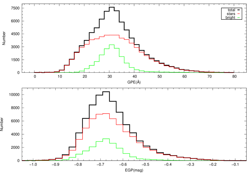
Figure 8.— Distribution of the saturation-corrected line indices, divided by source type as shown in the legend.

4. Selection of Metal-Poor Candidates

The saturation corrections described in Section 3.2 bring both source types of the second subsample to a common scale, so it is possible to apply a single set of restrictions for GPE and EGP to search for metal-poor stars based on carbon enrichment. This procedure is similar to the one adopted by Christlieb et al. (2001), who used a pair of carbon molecular indices (for CN and C₂) to find carbon-rich stars based on low-resolution spectra. The advantages of working with two indices defined in the same region of the spectra, but with different approaches in representing it, lies in the opportunity to identify likely spurious values, as discussed above.

4.1. Selection Criteria

The last step of the selection criteria has the goal of restricting the parameter space for the corrected line indices and provide a suitable subsample, both in absolute number and fraction of CEMP candidates, for the visual inspection. The second subsample contains 41,454 objects with GPE $>$ 31 Å and 42,823 objects with EGP $>$ $-$0.675, with 31,889 satisfying both conditions. It is interesting to note that for the sample in Paper I, only $\sim$7$\%$ of the stars were selected after the restriction in GPE. For the second subsample, this fraction is $\sim$51$\%$, even after the selection in the KP/color plane, which allows a more narrow index range to search for metal-poor stars.

In order to decrease the number of objects for visual inspection, another cut in (J$-$K)₀ was made, since the subsample has a great number of cool stars and we did not want to impose a more restrict criteria for the metallicity in the KP/color plane. as stated above. Besides that, for stars with (J$-$K)₀ $>$ 0.7, the accuracy of atmospheric parameters are limited in medium-resolution spectroscopy, mainly due to the low intensity of the Balmer lines used as auxilliary temperature indicators (Schörck et al., 2009), as well as the increasing saturation of the Ca ii K line.

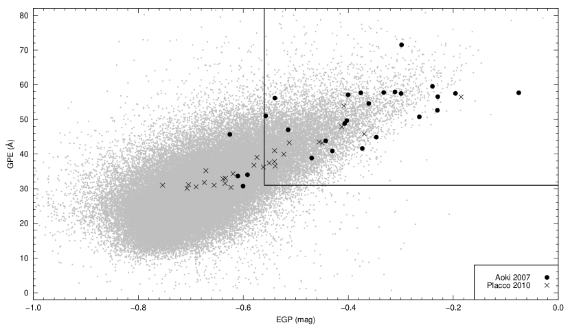
Figure 9.— Behavior of the line indices for the HES second subsample, along with the CEMP stars from the high-resolution spectroscopic follow-up of Aoki et al. (2007) , and the medium-resolution follow-up reported in Paper I. The solid lines represent the restrictions applied to the indices.

Figure 9 shows the behavior of the GPE and EGP indices for the second HES subsample stars with (J$-$K)₀ $<$ 0.7, along with the values for the low-resolution spectra of the CEMP stars ([Fe/H]$<-$1.0 and [C/Fe]$>+$1.0) from Aoki et al. (2007) and Paper I. The solid lines show the restrictions for the line indices. It is possible to see that some of the confirmed CEMP were left out of the selection window. This was a compromise between the number of candidates for visual inspection and the possible fraction of CEMP stars to be found within it.

The final restrictions applied to the line indices and color for the second subsample are: (i) GPE $>$ 31 Å; (ii) EGP $>$ $-$0.56 mag and; (iii) (J$-$K)₀ $<$ 0.7 mag. This set of constraints yielded 10,314 objects that were subjected to visual inspection, as described in the following subsection.

4.2. Visual Inspection

The visual inspection of the selected objects of the second subsample was carried out following the same methodology presented in Paper I, sorting the candidates based on spectral absorption features on the HES 1D spectra and digitized plates. The overall appearance of the object on the DSS direct plates was also inspected, to track down overlaps and plate artifacts. Besides that, no changes were made in the procedure due to the inclusion of bright sources, and the objects were divided into the same classes used in Christlieb et al. (2008) and Paper I.

4.2.1 Main Features and Results

The results of the inspection, and a brief description of the classes, are presented in Table 1. One can notice that the second subsample is dominated by stars with strong Ca ii K lines (mpcc), which is a direct reflection of the cumulative metallicity distribution function. There is also a great number of low-S/N spectra in the sample. This is due to the fact that there was no restriction made on the apparent magnitudes of the objects, in order to sample stars either more distant or less luminous, and also the outer regions of the Galaxy, including the dual halo components (Carollo et al., 2007, 2010, 2011). Moreover, the classes mpca, mpcb, and fhlc received a greater fraction of candidates than in Paper I, which means that the number of stars with [Fe/H] $<-$2.0 should increase when compared to the previous effort.

Another important point that arises from the quantities in Table 1 is the fact that there are only 3 objects, out of the over 10,000 inspected, presenting strong hydrogen lines (class habs). This is due, in part, to the (J$-$K)₀ $>$ 0.2 restriction, but mainly because of the combination of the GPE and EGP. As shown in Section 2, the relation of the line indices for objects with prominent hydrogen lines tends to be different then the one for the CEMP candidates, so this means that the restrictions imposed successfully filtered out these contaminations.

Figure 10 shows the distribution of the line indices for the inspected stars, excluding classes nois, ovl, and art. The remaining classes of Table 1 are evenly distributed about a linear relation between the line indices, with exception of mpca and mpcb, which are concentrated in the lower left region of the plot, along with the three objects associated with strong hydrogen lines. The stars with strong Ca ii K lines (mpcc) exhibit a wide range of index values. So, one can conclude that these objects would present a variety of [C/Fe] values, and also [Fe/H] values, since even cool giant stars with [Fe/H] $\sim-$2.0 exhibit strong Ca lines (Schörck et al., 2009). In addition, when comparing Figure 10 with the same region in Figure 9, one can note a clear trend between the line indices, and the objects located far from this trend (i.e., GPE $<$ 40 Å and EGP $>$ 0.3 mag) have spectra associated with the classes excluded from the plot, with spurious values for the indices.

Table 1Visual Inspection Classification for the Selected Candidates

Tag	Description	Candidates
mpca	Absent Ca ii K line	55
mpcb	Weak Ca ii K line	452
mpcc	Strong Ca ii K line	5184
unid	Ca ii K line not found	224
fhlc	Faint high latitude carbon stars	317
habs	Strong absorption H lines	3
hbab	Horizontal-branch/$A$ type star	0
nois	Low signal-to-noise ratio	2320
ovl	Overlapping spectra	1038
art	Artifacts on photographic plates	721

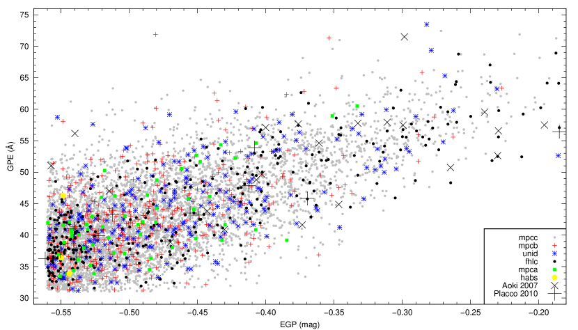
Figure 10.— Results of the visual inspection of the candidates, according to the classes described in Table 1.

4.2.2 Comparison with Paper I

We also wish to test the efficiency of our new search procedure, using the GPE and the EGP indices, by comparing the results of the visual inspection with the one made in Paper I. This can be done by calculating the effective fractions of the various types of objects identified, excluding the classes art, nois and ovl. Results are shown in Table 2. Some interesting aspects of the visual inspection can arise from the analysis of the fractions presented: (i) the “clean” samples present a similar number of candidates, but the one associated with this work does not have magnitude restrictions. This removes the brightness and/or distance related bias introduced in Paper I due to observational limitations; (ii) the fractions associated with the mpcc class for both subsamples are similar, suggesting that those stars are evenly distributed in the parameter space associated with the visual inspections; and (iii) for the mpca and fhlc classes, the fractions increased by an order of magnitude in comparison to the Paper I sample. These candidates form a set of stars with high probabilities of occurance of EMP ([Fe/H] $<-$ 3.0) carbon-rich stars; (iv) the objects with intense hydrogen lines (habs and hbab), considered a contamination on the first subsample, were (with the exception of three objects) removed from the second subsample by the method based on the combination of line indices and by the restriction imposed in (J$-$K)₀ color; and (v) the objects associated with the mpcb and unid classes presented an increase of about $\sim$30% in their effective fractions.

Table 2Comparison Between Visual Inspections

	Paper I sample		This work
Class	$n$	fraction	$n$	fraction
mpca	4	0.07$\%$	55	0.88$\%$
mpcb	293	5.32$\%$	452	7.25$\%$
mpcc	4711	85.58$\%$	5184	83.14$\%$
fhlc	31	0.56$\%$	317	5.08$\%$
unid	155	2.81$\%$	224	3.60$\%$
hbab	235	4.28$\%$	0	0.00$\%$
habs	76	1.38$\%$	3	0.05$\%$
Total	5505	100$\%$	6235	100$\%$

Finally, a search in the literature was made in order to exclude objects already observed or classified by other studies. Among the 6,235 stars shown in Figure 10, 5,288 do not appear in any study to date. A table with relevant information on these stars is available electronically, and its parameters are listed in Appendix A.

5. Follow-up Observations of Selected Candidates

To validate the analysis of our selected candidates, especially for the saturation-corrected bright sources, we have obtained medium-resolution spectra for a limited number of metal-poor candidates with the SOAR 4.1m and Gemini 8m telescopes. After gathering and reducing the data, we obtained estimates of the stellar atmospheric parameters using the n-SSPP, a modified version of the SEGUE Stellar Parameter Pipeline (SSPP - see Lee et al., 2008a, b; Allende Prieto et al., 2008; Smolinski et al., 2011; Lee et al., 2011, for a detailed description of the procedures used). The carbon abundances ([C/Fe]), were obtained using spectral synthesis. Further details are provided below.

5.1. Spectroscopic Observations and Stellar Data

The observed sample consists of data collected with two different telescope/spectrograph combinations: SOAR/Goodman and Gemini/GMOS. The addition of Gemini observations were of great interest, specifically to increase the magnitude limit reached by our program to B$\sim$16.0, with exposure times no longer than 30 minutes. Accordingly, the brighter sources were observed preferentially with SOAR.

The 58 star sample from SOAR consists of data observed in the 2009B, 2010B and 2011A semesters. All the observations were carried out with the Goodman Spectrograph, using the 600 l mm^-1 grating in the blue setting with a 1$\farcs$03 slit, covering the wavelength range 3550-5500 Å. This combination yielded a resolving power of $R\sim 1500$ and sufficient signal-to-noise ratios (S/N$\sim 40$ per pixel at 4300 Å). GMOS data for the 59 stars from Gemini North and South were gathered in 2010A and 2011A, observed in Bands 3 and 4. The setup was similar to the one used in SOAR, with a 600 l mm^-1 grating in the blue setting (G5323 for GMOS South and G5307 for GMOS North) and a 1$\farcs$00 slit. The resolving power ($R\sim 1700$) and signal-to-noise ratios (S/N$\sim 40$ per pixel at 4300 Å) of these spectra are also suitable to determine atmospheric parameters and carbon abundances.

For both SOAR and Gemini data, the calibration frames included HgAr and Cu arc lamp exposures (taken following each science observation), biases frames, and quartz flats. All tasks related to calibration and spectral extraction were performed using standard IRAF packages. Table 3 lists the equatorial coordinates, BHES magnitude, (J$-$K)₀, GPE, EGP, telescope and target classification (according to Table 1) for the 117 observed candidates.

5.2. Atmospheric Parameters, [C/Fe] and CEMP Candidates

The atmospheric parameters and carbon abundances were determined with the same procedures used in Paper I. Given the improvements of the n-SSPP over the last two years, we decided to reprocess the data for the first sample, in order to produce a more homogeneous set of parameters.

Figure 11 shows the residual distribution of [Fe/H], $T_{\rm eff}$ , and log $g$  as a function of the latest estimates. The residuals for the metallicity spread between $-$0.5 and 0.5 dex for [Fe/H] $<-$1.0, and there is a strong positive trend for the new calculations on the metal-rich end. These new values of [Fe/H] also reflect on the [C/Fe], since the estimated values of [C/H] did not change. For the temperature residuals there are some values outside the [$-$500 K:$+$500 K] range, and for log $g$  there is an underlying positive linear trend for increasing values. These changes are mainly due to new calibrations implemented on the code, and extensive testing was performed to assure the quality of the new determinations.

Figure 11.— Residual distribution of the atmospheric parameters for the Paper I sample, reprocessed with the latest version of the n-SSPP. The trends represent recent improvements made to the n-SSPP.

The atmospheric parameter estimates for the observed metal-poor candidates presented in Table 3 were also obtained via the n-SSPP; results are listed in Table 4. The last column refers to the carbon-to-iron abundance ratios ([C/Fe]; “carbonicity”), obtained with the same procedure described in Paper I, using spectral synthesis in the G-band region. Updated results for the sample from Paper I are also shown in the table. Typical errors for the atmospheric parameters are 0.3 dex for [Fe/H], 300 K for $T_{\rm eff}$  and 0.4 for log $g$ . The errors associated with the carbonicity are, on average, 0.2 dex.

Figure 12 shows the behavior of carbonicity as a function of metallicity for the stars observed in this work, as well as from the medium-resolution data of Paper I, high-resolution spectroscopic data from Aoki et al. (2007) and Caffau et al. (2011), and for stars with [Fe/H]$<-2.5$ retrieved from the SAGA database (Stellar Abundances for Galactic Archeology - Suda et al., 2008). The left and lower panels show the distributions of [Fe/H] and [C/Fe] for the stars of this work and Paper I. It can be seen that the new selection criteria successfully sampled the [Fe/H]$<-$3.0 region, with essentially all stars in this range presenting [C/Fe] $>+$1.0, including two stars with remarkably high carbonicity ([C/Fe] $\geq+$2.90). We also reproduce the strong signature of increasing [C/Fe] with declining [Fe/H] reported by previous work. The increasing scatter in [C/Fe] at lower metallicities cannot be accounted for by uncertainties in the carbonicity determinations, rather it is likely due to the presence of multiple nucleosynthesis paths that produce carbon at low metallicity (Cescutti & Chiappini, 2010). The features presented by this group of stars are also consistent with the latest studies regarding the relationship between the carbonicity and metallicity with the structural components of the Milky Way. According to Carollo et al. (2011), the CEMP stars with metallicity [Fe/H] $<-2.5$ have a high probability of belonging to the outer-halo component of the Galaxy. Future high-resolution spectroscopic follow-up of these stars can help shed light on the matter.

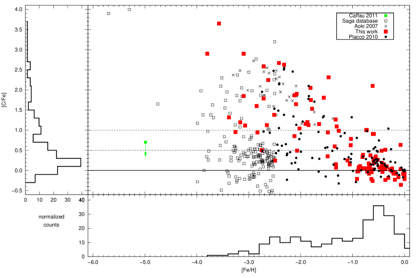
Figure 12.— Carbonicity, [C/Fe], as a function of the metallicity, [Fe/H], for the stars observed in this work, compared with data from the high-resolution spectroscopic follow-up of Aoki et al. (2007) and Caffau et al. (2011), from the SAGA database and from the medium-resolution follow-up of Paper I. The solid line is the [C/Fe] = 0.0 level, the long dashed line is the [C/Fe] = $+$0.5 level, and the short dashed line is the [C/Fe] = $+$1.0 level. The left and bottom panels show the marginalized distributions for each quantity, related to the data from this work and Paper I.

Even with the observation of a number of solar-metallicity stars, it is clear from inspection of Figure 12 that the new selection criteria is successful in the discovery of VMP and EMP stars. This is mainly due to the GPE and EGP cuts shown in Figure 9. By taking the index values for the stars from SAGA database in Figure 12 with low-resolution counterparts in the HES database, it can be seen that roughly 70% of the confirmed CEMP stars ([Fe/H] $<-1.0$ and [C/Fe] $>+1.0$) fall into the selection area (GPE$>$ 31 Å and EGP $>$ -0.56 mag).

Figure 13 illustrates two of the most interesting new discoveries of our new approach, comparing the low-resolution HES spectra (subject to visual inspection) with data from SOAR and Gemini medium-resolution spectroscopy. HE 1046$-$1352 (left panels) was selected after combining the two line indices and separating the $mpca$ candidates by visual inspection. The right panels of Figure 13 show HE 1937$-$6314. This object was selected after inclusion of the bright sources (its BHES apparent magnitude is 13.6) and subsequent saturation corrections of the line indices, and it is not the subject of any previous study. Stars of this sort are of special interest, since their apparent magnitudes permit shorter exposures for high-resolution spectroscopic studies.

Figure 13.— Comparison between low-resolution HES spectra and the medium-resolution spectra acquired with SOAR and Gemini. The main features assessed by visual inspection are labeled in the upper panels. HE 1046$-$1352 has BHES = 15.3, while HE 1937$-$6314 has BHES = 13.6.

6. Conclusions

One of the goals of this work was to discover additional CEMP stars (which are in turn often of very low metallicity) still hiding in the scanned photographic plates and low-resolution spectra of the HES. To accomplish this, we extended the approach taken in Paper I to include bright sources in the selection criteria applied to the database.

Line indices and corrections for the bright sources were developed specifically for the HES data, in order to compensate for the saturation effects presented by these spectra. These will be included in the full stellar database, to help in future searches for bright CEMP and metal-poor stars. Moreover, the introduction of this new set of carbon line indices for low-resolution spectroscopy can be easily adapted and implemented to help pre-process and select interesting targets for follow-up spectroscopy in the massive amount of data coming from the next generation of large surveys. The use of an auxilliary index to search for CEMP candidates successfully filtered out some unwanted objects, and increased the relative number of the most interesting classes of metal-poor stars (see Table 2).

Medium-resolution spectroscopy with the SOAR and Gemini telescopes revealed an improvement in our ability to isolated the targets of greatest interest relative to Paper I. Comparing the stars of this work lying in the same magnitude range as the targets from Paper I ($13.9\leq{\rm BHES}\leq 15.1$), the fractions of low-metallicity stars found increased from 53% to 58% for [Fe/H] $<-1.0$, from 27% to 32% for [Fe/H] $<-2.0$ and from 7% to 21% for [Fe/H] $<-2.5$, an improvement by a factor of 3 in this last metallicity range. Our observations of the newly identified sample of low-metallicity candidates has contributed eight new stars with [Fe/H] $<-3.0$.

Regarding the carbonicity of our targets, over the entire magnitude range observed by our program ($10.5\leq{\rm BHES}\leq 16.0$), a total of about 40% were shown to possess [Fe/H] $<-1.0$ (85% of these with [C/Fe] $>+0.5$, 65% with [C/Fe] $>+1.0$); 21% with [Fe/H] $<-2.0$ (92% of these with [C/Fe] $>+0.5$, 76% with [C/Fe] $>+1.0$), and 7% with [Fe/H] $<-3.0$ (100% of these with [C/Fe] $>+0.5$, 88% with [C/Fe] $>+1.0$). The combined sample of this work and Paper I contains 234 CEMP/metal-poor star candidates with available medium-resolution spectroscopy, including 108 stars with [Fe/H] $<-1.0$ (74 stars with [C/Fe] $>+0.5$, 51 with [C/Fe] $>+1.0$), 57 with [Fe/H] $<-2.0$ (43 stars with [C/Fe] $>+0.5$, 32 with [C/Fe] $>+1.0$), and 8 with [Fe/H] $<-3.0$ (8 stars with [C/Fe] $>+0.5$, 7 with [C/Fe] $>+1.0$). These numbers are important to increase the current statistics on CEMP stars, since the lack of carbon abundance data in specific regimes (especially for [Fe/H] $<-$3.0), limits our ability to distinguish between statistical and cosmic scatter in the [Fe/H] vs. [C/Fe] plane. As mentioned in the Introduction, we expect this very low-metallicity range to be dominated by the CEMP-no class objects, which may provide important clues to the nucleosynthesis products of the first generations of stars.

The visual inspection described in Section 4.2 also generated a list of 5,288 CEMP star candidates to serve as inputs for our continued medium-resolution spectroscopic follow-up, which aims in particular at increasing the numbers of known extremely metal-poor stars selected on the basis of their strong carbon enhancements. The CEMP stars identified in the range $-2.0\leq$ [Fe/H]$\leq-1.0$, which we expect to be dominated by the CEMP-s class, supplement the intermediate-metallicity region, which has been undersampled by previous follow-up efforts directed primarily at lower metallicities.

It is important to recognize that our sample of newly discovered CEMP stars is not suitable for estimation of CEMP star fractions in the Galaxy, due to its selection on carbon in the first place. There are other, much larger and non carbon-biased samples, for which this exercise can be carried out. Carollo et al. (2011) have done this for the SDSS/SEGUE calibration stars through SDSS DR7. Their analysis indicates a significant difference in the CEMP star fractions between the inner- and outer-halo components, so a discussion of the global fractions of CEMP stars with metallicity no longer appears to be the most pressing question. More careful attention will also have to be paid in the future to the issue of the detectability of the CH G-band feature with increasing effective temperature, which results in most previous estimates of the CEMP star fractions in reality being lower limits. Studies of the kinematics of our sample are planned, once the number of stars with available medium-resolution spectroscopy increases. This information can be used to seek assignment of the thick-disk, metal-weak thick-disk, or inner/outer-halo status for our program stars. Finally, high-resolution spectroscopic follow-up of our program stars, in particular the VMP and EMP stars with enhanced carbonicity, will enable their assignment into the appropriate subclasses of CEMP stars.

Table 3Stellar Data for the Observed Candidates

Name	$\alpha$(J2000)	$\delta$(J2000)	BHES	(J$-$K)0	GPE(Å)	EGP(mag)	Telescope	Tag
HE 0002$-$1037	00:05:23.0	$-$10:20:25	14.6	0.55	52.1	$-$0.41	SOAR	fhlc
HE 0004$-$2546	00:06:33.1	$-$25:29:21	11.3	0.58	18.8	$-$0.67	SOAR	mpcc
HE 0020$-$2549	00:22:39.0	$-$25:32:58	11.6	0.66	23.9	$-$0.67	SOAR	mpcc
HE 0046$-$4712	00:48:57.0	$-$46:55:57	15.0	0.44	35.4	$-$0.47	SOAR	mpcc
HE 0055$-$2507	00:57:56.4	$-$24:51:07	11.3	0.63	22.3	$-$0.66	SOAR	mpcc
HE 0059$-$6540	01:01:18.1	$-$65:23:56	14.6	0.56	36.8	$-$0.54	SOAR	fhlc
HE 0113$-$3806	01:16:11.8	$-$37:50:24	15.1	0.30	41.0	$-$0.54	SOAR	mpcb
HE 0123$+$0023	01:26:30.4	$+$00:39:13	15.0	0.26	29.4	$-$0.70	SOAR	unid
HE 0134$-$2504	01:36:37.3	$-$24:49:03	15.3	0.45	55.6	$-$0.30	SOAR	fhlc
HE 0317$-$4705	03:18:45.2	$-$46:54:39	13.7	0.65	39.6	$-$0.46	SOAR	fhlc
HE 0515$-$3358	05:17:08.3	$-$33:55:03	14.6	0.62	31.6	$-$0.53	GEMINI	mpcc
HE 0532$-$3819	05:33:50.8	$-$38:17:07	15.0	0.55	38.2	$-$0.47	GEMINI	fhlc
HE 0546$-$4421	05:48:15.6	$-$44:20:37	11.8	0.67	27.1	$-$0.60	SOAR	fhlc
HE 0548$-$4508	05:50:21.0	$-$45:07:43	12.0	0.59	35.1	$-$0.49	GEMINI	fhlc
HE 0854$+$0105	08:57:12.6	$+$00:53:55	16.0	0.58	55.3	$-$0.28	GEMINI	fhlc
HE 0911$+$0011	09:14:16.5	$+$00:01:08	15.4	0.36	53.1	$-$0.43	GEMINI	mpcc
HE 0919$-$0049	09:22:24.1	$-$01:02:04	16.0	0.43	48.3	$-$0.44	GEMINI	unid
HE 0923$-$0016	09:26:17.8	$+$00:29:13	15.2	0.41	38.7	$-$0.51	GEMINI	mpcc
HE 0927$-$0035	09:30:10.8	$+$00:48:19	11.2	0.67	17.0	$-$0.68	SOAR	fhlc
HE 0930$-$1047	09:33:06.4	$-$11:00:53	15.8	0.49	46.0	$-$0.40	GEMINI	mpcb
HE 0932$+$0005	09:35:03.5	$+$00:08:17	15.1	0.58	52.8	$-$0.37	SOAR	fhlc
HE 0932$-$0838	09:34:36.6	$-$08:52:08	15.8	0.32	47.1	$-$0.42	GEMINI	mpcc
HE 0942$-$0446	09:44:42.2	$-$05:00:24	15.8	0.34	49.2	$-$0.41	GEMINI	mpcc
HE 0943$-$0227	09:46:14.0	$-$02:40:57	13.6	0.37	35.1	$-$0.55	GEMINI	fhlc
HE 0946$-$0737	09:48:45.4	$-$07:51:14	15.9	0.37	45.4	$-$0.45	GEMINI	mpcc
HE 0954$+$0219	09:56:48.9	$+$02:05:20	14.3	0.67	43.9	$-$0.46	SOAR	fhlc
HE 0954$-$0744	09:56:29.7	$-$07:59:10	15.1	0.42	31.2	$-$0.53	GEMINI	mpcc
HE 1006$-$1237	10:08:48.2	$-$12:52:24	15.2	0.31	43.8	$-$0.58	GEMINI	unid
HE 1007$-$1343	10:09:50.2	$-$13:58:08	15.6	0.33	48.3	$-$0.47	GEMINI	unid
HE 1013$-$1648	10:15:40.6	$-$17:03:53	15.7	0.47	48.7	$-$0.52	GEMINI	unid
HE 1016$-$1625	10:19:11.6	$-$16:40:47	15.6	0.45	48.7	$-$0.48	GEMINI	mpcb
HE 1022$-$0730	10:24:39.3	$-$07:45:59	14.9	0.37	28.9	$-$0.58	GEMINI	mpcb
HE 1022$-$1621	10:24:40.5	$-$16:36:57	15.6	0.39	46.1	$-$0.54	GEMINI	unid
HE 1027$-$1217	10:29:29.9	$-$12:32:31	15.1	0.43	32.2	$-$0.67	GEMINI	mpcb
HE 1029$-$1757	10:31:55.3	$-$18:12:42	14.0	0.45	37.5	$-$0.46	GEMINI	fhlc
HE 1032$-$1809	10:35:18.8	$-$18:25:01	15.5	0.67	58.0	$-$0.28	GEMINI	fhlc
HE 1032$-$2042	10:35:06.9	$-$20:57:54	15.9	0.40	46.9	$-$0.53	GEMINI	mpcc
HE 1034$-$1632	10:36:56.4	$-$16:48:08	15.2	0.34	37.1	$-$0.68	GEMINI	mpcc
HE 1035$-$1603	10:37:38.7	$-$16:18:44	15.6	0.59	50.5	$-$0.30	GEMINI	unid
HE 1037$-$0301	10:39:40.1	$-$03:17:08	15.8	0.48	52.5	$-$0.38	GEMINI	mpcc
HE 1040$-$1957	10:42:59.4	$-$20:12:54	15.9	0.63	48.2	$-$0.43	GEMINI	unid
HE 1042$-$1107	10:44:58.5	$-$11:23:15	16.0	0.42	45.8	$-$0.56	GEMINI	unid
HE 1043$-$1516	10:45:51.0	$-$15:32:23	15.6	0.61	53.2	$-$0.31	GEMINI	fhlc
HE 1045$-$1313	10:48:15.3	$-$13:29:01	16.0	0.40	45.2	$-$0.36	GEMINI	unid
HE 1046$-$1352	10:48:29.9	$-$14:08:12	15.3	0.47	52.1	$-$0.41	GEMINI	mpca
HE 1047$-$1140	10:49:41.6	$-$11:56:15	15.2	0.59	45.7	$-$0.48	GEMINI	unid
HE 1053$-$2017	10:56:25.3	$-$20:33:04	15.8	0.62	55.3	$-$0.32	GEMINI	mpcc
HE 1054$-$2718	10:57:06.7	$-$27:34:30	15.9	0.30	58.9	$+$0.08	GEMINI	mpcc
HE 1055$-$2647	10:57:29.0	$-$27:03:50	13.8	0.69	30.4	$-$0.49	SOAR	mpcc
HE 1106$-$0725	11:09:28.6	$-$07:41:20	16.0	0.40	45.8	$-$0.54	GEMINI	mpcb
HE 1110$-$2529	11:13:04.1	$-$25:45:59	15.6	0.68	59.8	$-$0.23	GEMINI	fhlc
HE 1111$-$2817	11:14:09.4	$-$28:33:36	16.0	0.45	45.6	$-$0.39	GEMINI	mpcb
HE 1111$-$3026	11:13:45.0	$-$30:42:48	15.6	0.53	51.7	$-$0.32	GEMINI	fhlc
HE 1112$-$1140	11:15:14.5	$-$11:56:50	11.4	0.65	16.2	$-$0.65	SOAR	mpcc
HE 1124$-$2343	11:26:56.2	$-$23:59:53	11.2	0.57	20.5	$-$0.68	SOAR	mpcc
HE 1126$-$1229	11:28:48.5	$-$12:46:07	10.9	0.65	15.2	$-$0.67	SOAR	fhlc
HE 1134$-$1731	11:37:11.4	$-$17:47:45	15.4	0.54	53.6	$-$0.27	GEMINI	unid
HE 1140$-$2814	11:43:03.2	$-$28:31:02	11.8	0.61	14.5	$-$0.64	SOAR	fhlc
HE 1141$-$3140	11:43:51.7	$-$31:57:35	10.5	0.67	18.1	$-$0.65	SOAR	fhlc
HE 1142$-$1058	11:44:45.9	$-$11:14:56	14.8	0.30	45.8	$-$0.44	GEMINI	mpcc
HE 1144$-$2555	11:46:46.7	$-$26:12:09	15.8	0.39	45.2	$-$0.51	GEMINI	mpcc
HE 1146$-$1040	11:49:24.5	$-$10:56:41	15.0	0.50	41.2	$-$0.48	GEMINI	mpcc
HE 1146$-$1128	11:48:47.7	$-$11:44:47	14.7	0.33	32.5	$-$0.64	GEMINI	unid
HE 1147$-$0415	11:50:30.0	$-$04:32:14	15.5	0.47	43.9	$-$0.41	GEMINI	fhlc
HE 1150$-$2800	11:53:26.2	$-$28:17:03	16.0	0.42	46.3	$-$0.38	GEMINI	fhlc
HE 1153$-$2326	11:55:58.7	$-$23:43:03	16.0	0.34	46.9	$-$0.53	GEMINI	mpcb
HE 1202$-$2732	12:05:20.2	$-$27:48:52	15.3	0.60	54.3	$-$0.28	GEMINI	fhlc
HE 1216$-$0739	12:18:39.6	$-$07:55:39	15.0	0.41	40.8	$-$0.49	GEMINI	unid
HE 1233$-$2435	12:36:14.9	$-$24:52:27	15.9	0.46	49.6	$-$0.56	GEMINI	unid
HE 1254$-$2320	12:56:48.4	$-$23:36:29	16.0	0.38	51.8	$-$0.45	GEMINI	unid
HE 1304$-$1128	13:07:01.8	$-$11:44:23	15.9	0.51	52.1	$-$0.36	GEMINI	mpcc
HE 1315$-$2807	13:18:34.2	$-$28:23:02	12.5	0.65	31.4	$-$0.57	SOAR	fhlc
HE 1328$-$1740	13:31:22.8	$-$17:56:21	15.2	0.46	44.4	$-$0.34	GEMINI	mpcc
HE 1329$-$2347	13:32:03.2	$-$24:02:57	16.0	0.60	41.3	$-$0.52	GEMINI	mpca
HE 1336$-$1832	13:39:38.0	$-$18:47:21	12.5	0.67	25.0	$-$0.56	SOAR	fhlc
HE 1337$-$2608	13:39:49.2	$-$26:24:10	15.6	0.38	37.8	$-$0.64	GEMINI	unid
HE 1342$-$2731	13:44:53.1	$-$27:46:38	11.2	0.64	17.6	$-$0.67	SOAR	mpcc
HE 1343$-$0626	13:45:53.5	$-$06:41:28	15.5	0.42	48.3	$-$0.51	GEMINI	mpcc
HE 1348$-$3057	13:51:05.3	$-$31:12:28	14.8	0.64	60.2	$-$0.20	GEMINI	fhlc
HE 1350$-$2422	13:53:33.9	$-$24:37:17	13.7	0.60	35.5	$-$0.45	SOAR	fhlc
HE 1350$-$2734	13:53:09.5	$-$27:49:14	14.5	0.68	36.2	$-$0.42	GEMINI	fhlc
HE 1401$-$1236	14:03:41.9	$-$12:50:39	15.9	0.43	46.9	$-$0.44	GEMINI	mpcc
HE 1428$-$1950	14:30:59.4	$-$20:03:42	13.1	0.62	33.8	$-$0.48	SOAR	fhlc
HE 1444$-$1219	14:47:15.6	$-$12:31:45	15.1	0.57	29.1	$-$0.64	SOAR	mpcb
HE 1501$-$0858	15:03:46.2	$-$09:10:12	12.0	0.64	20.4	$-$0.63	SOAR	mpcc
HE 1503$-$0918	15:05:50.9	$-$09:30:24	14.8	0.35	37.1	$-$0.54	SOAR	unid
HE 1507$-$1122	15:10:09.9	$-$11:33:20	10.6	0.66	17.2	$-$0.67	SOAR	fhlc
HE 1508$-$0736	15:11:15.8	$-$07:47:30	14.9	0.28	30.2	$-$0.61	SOAR	mpcc
HE 1509$-$1437	15:12:30.3	$-$14:48:15	11.8	0.66	18.6	$-$0.61	SOAR	mpcb
HE 1514$-$0943	15:17:36.0	$-$09:53:59	15.2	0.31	35.1	$-$0.57	GEMINI	mpcb
HE 1516$-$0903	15:18:58.4	$-$09:14:38	12.8	0.66	30.7	$-$0.55	SOAR	mpcc
HE 1523$-$1155	15:26:41.0	$-$12:05:43	14.6	0.55	52.5	$-$0.23	SOAR	fhlc
HE 1937$-$6314	19:42:00.7	$-$63:06:57	13.6	0.52	43.0	$-$0.37	SOAR	fhlc
HE 1939$-$6626	19:44:38.8	$-$66:18:49	13.7	0.67	27.6	$-$0.46	SOAR	fhlc
HE 2006$-$5334	20:10:20.7	$-$53:25:52	15.0	0.85	40.5	$-$0.35	SOAR	unid
HE 2030$-$5323	20:33:53.3	$-$53:13:17	14.3	0.53	28.9	$-$0.60	SOAR	mpcb
HE 2030$-$6056	20:34:59.8	$-$60:45:42	12.3	0.70	24.5	$-$0.58	SOAR	mpcc
HE 2033$-$6206	20:37:44.3	$-$61:55:43	14.7	0.32	34.9	$-$0.52	SOAR	mpcc
HE 2043$-$5525	20:47:02.1	$-$55:14:39	14.8	0.55	41.7	$-$0.47	SOAR	mpcc
HE 2056$-$6128	21:00:03.4	$-$61:17:05	15.0	0.41	34.0	$-$0.62	SOAR	mpcc
HE 2118$-$5654	21:22:19.9	$-$56:41:12	14.9	0.47	41.0	$-$0.54	SOAR	mpcc
HE 2121$-$5308	21:25:20.6	$-$52:55:41	13.3	0.64	34.8	$-$0.49	SOAR	fhlc
HE 2125$-$3447	21:28:04.0	$-$34:33:57	13.5	0.69	27.6	$-$0.49	SOAR	fhlc
HE 2134$-$0637	21:37:01.3	$-$06:23:39	15.0	0.35	29.8	$-$0.70	SOAR	unid
HE 2135$-$0759	21:38:17.0	$-$07:46:10	11.3	0.69	13.5	$-$0.68	SOAR	fhlc
HE 2136$-$5928	21:40:08.0	$-$59:14:31	15.2	0.46	39.1	$-$0.48	SOAR	fhlc
HE 2138$-$5620	21:42:08.5	$-$56:06:49	15.0	0.62	30.0	$-$0.63	SOAR	mpcc
HE 2146$-$0247	21:49:06.8	$-$02:33:45	15.1	0.58	30.4	$-$0.67	SOAR	mpcc
HE 2148$-$1058	21:50:44.9	$-$10:44:49	10.7	0.65	13.9	$-$0.68	SOAR	fhlc
HE 2151$-$0643	21:54:08.6	$-$06:29:29	15.1	0.33	25.6	$-$0.70	SOAR	mpcc
HE 2155$-$3750	21:58:09.7	$-$37:36:20	14.1	0.50	40.8	$-$0.46	SOAR	fhlc
HE 2200$-$1146	22:03:05.9	$-$11:32:07	15.1	0.35	28.7	$-$0.72	SOAR	mpcb
HE 2211$-$1806	22:14:23.9	$-$17:51:28	15.3	0.44	57.6	$-$0.29	SOAR	fhlc
HE 2220$-$2250	22:22:57.8	$-$22:35:42	11.5	0.65	14.5	$-$0.67	SOAR	mpcc
HE 2229$-$1619	22:32:35.0	$-$16:04:15	15.1	0.52	41.7	$-$0.49	SOAR	mpcc
HE 2324$-$0424	23:26:58.9	$-$04:08:23	14.6	0.46	34.6	$-$0.64	SOAR	mpcb
HE 2339$-$3236	23:42:07.0	$-$32:19:26	14.3	0.58	32.0	$-$0.58	SOAR	fhlc

Table 4Atmospheric Parameters and Carbonicity Estimates for the Observed Candidates.

Name	V (km/s)	$T_{\rm eff}$  (K)	log $g$  (cgs)	[Fe/H]	[C/Fe]
HE 0002$-$1037	$-$73.0	4895	3.09	$-$3.07	$+$1.12
HE 0004$-$2546	31.2	4916	4.01	$-$0.59	$+$0.18
HE 0008$+$0049	$-$12.4	4862	3.56	$-$1.27	$-$0.32
HE 0020$-$2549	25.6	5078	2.74	$-$0.91	$-$0.03
HE 0024$-$0550	17.8	5538	2.98	$-$1.78	$+$0.31
HE 0034$-$0011	$-$218.8	5934	2.52	$-$1.74	$+$1.71
HE 0035$-$5803	30.6	5807	3.75	$-$0.70	$+$0.47
HE 0046$-$4712	$-$119.0	5340	3.62	$-$1.04	$+$0.63
HE 0053$-$0356	$-$86.2	5752	2.21	$-$1.84	$+$1.85
HE 0055$-$2507	35.9	4895	3.29	$-$0.34	$+$0.09
HE 0058$+$0141	$-$48.4	6271	4.08	$-$0.68	$+$0.48
HE 0059$-$6540	$-$28.4	4727	1.00	$-$3.17	$+$1.20
HE 0100$-$4957	126.9	5970	3.54	$-$1.03	$+$0.28
HE 0102$-$0004	$-$191.6	5814	3.45	$-$2.45	$+$0.64
HE 0113$-$3806	$-$131.2	5886	3.14	$-$2.08	$+$1.90
HE 0118$-$4834	$-$144.2	5609	2.27	$-$2.42	$+$2.14
HE 0123$+$0023	$-$304.0	6322	2.97	$-$1.81	$+$2.05
HE 0134$-$2504	$-$41.5	5150	2.42	$-$3.10	$+$1.85
HE 0156$-$5608	213.7	5137	4.27	$-$2.00	$+$0.47
HE 0159$-$5216	$-$18.1	5117	1.85	$-$2.03	$+$0.78
HE 0214$-$0818	$-$48.6	6177	2.85	$-$1.02	$+$1.32
HE 0307$-$5339	163.0	5465	2.45	$-$2.14	$+$1.34
HE 0316$-$2903	198.2	5795	3.15	$-$1.56	$+$1.35
HE 0317$-$4705	173.5	4231	3.06	$-$3.26	$+$0.95
HE 0320$-$1242	44.6	5749	4.17	$-$0.43	$+$0.18
HE 0322$-$3720	$-$38.5	4660	4.55	0.00	$+$0.02
HE 0336$-$3948	101.4	5952	3.86	$-$0.53	$+$0.28
HE 0340$-$3933	$-$67.1	5991	4.03	$-$0.04	$+$0.01
HE 0345$+$0006	$-$51.2	5199	2.61	$-$2.74	$+$0.49
HE 0405$-$4411	45.0	6180	3.55	$-$1.23	$+$0.85
HE 0414$-$4645	38.5	5820	3.78	$-$1.08	$+$0.33
HE 0440$-$5525	26.2	6361	3.65	$-$0.52	$+$0.47
HE 0444$-$3536	117.0	5197	2.42	$-$1.66	$+$0.96
HE 0449$-$1617	70.6	5766	4.42	$-$0.30	$-$0.14
HE 0451$-$3127	305.2	5505	1.85	$-$2.43	$+$1.49
HE 0500$-$5603	99.6	5808	3.67	$-$0.56	$+$0.19
HE 0509$-$1611	92.9	5108	3.05	$-$0.49	$-$0.01
HE 0511$-$3411	50.6	5873	4.04	$-$0.38	$+$0.16
HE 0514$-$5449	119.2	6505	4.19	$-$0.55	$+$0.28
HE 0515$-$3358	16.6	5057	1.99	$-$0.60	$+$0.26
HE 0518$-$3941	18.4	6562	3.36	$-$0.56	$+$0.58
HE 0532$-$3819	$-$40.6	5031	1.69	$-$1.48	$+$0.94
HE 0535$-$4842	32.1	5935	4.30	$-$0.58	$+$0.25
HE 0536$-$5647	89.5	5639	4.08	$-$0.46	$-$0.16
HE 0537$-$4849	30.9	5082	4.73	$-$0.38	$+$0.13
HE 0546$-$4421	11.5	4966	4.87	0.00	$-$0.17
HE 0548$-$4508	51.1	5163	1.05	$-$2.42	$+$2.67
HE 0854$+$0105	$-$13.7	4951	2.10	$-$0.72	$-$0.03
HE 0901$-$0003	$-$4.0	5077	4.14	$-$0.26	$+$0.01
HE 0910$-$0126	112.3	6409	3.24	$-$2.00	$+$0.92
HE 0911$+$0011	$-$64.1	5554	4.04	$-$0.73	$+$0.05
HE 0912$+$0200	78.4	5003	4.12	$-$0.06	$+$0.07
HE 0918$-$0156	65.9	4114	2.34	$-$0.99	$-$0.01
HE 0919$-$0049	$-$11.9	5609	3.88	$-$0.35	$+$0.10
HE 0923$-$0016	$-$10.9	5929	3.49	$-$1.27	$+$0.98
HE 0923$-$0323	57.7	5576	3.67	$-$0.74	$+$0.28
HE 0927$-$0035	86.4	4737	3.09	$-$0.43	$-$0.03
HE 0928$+$0059	$-$61.3	6482	3.67	$-$0.60	$+$0.54
HE 0930$-$1047	$-$17.7	5387	4.14	$-$1.06	$+$0.15
HE 0932$+$0005	$-$4.1	4816	4.81	$-$0.86	$+$0.11
HE 0932$-$0838	$-$44.9	5648	3.10	$-$0.56	$+$0.35
HE 0933$-$0733	20.2	5444	4.10	$-$1.04	$+$0.21
HE 0942$-$0446	$-$70.8	5919	3.91	$-$0.07	$+$0.03
HE 0943$-$0227	11.5	5833	3.32	$-$0.37	$+$0.51
HE 0946$-$0737	$-$64.5	5433	4.41	$-$0.67	$+$0.12
HE 0948$+$0107	442.5	5081	3.88	$-$2.27	$-$0.23
HE 0948$-$0234	114.5	5807	4.07	$-$1.02	$+$0.41
HE 0950$-$0401	90.4	5849	3.62	$-$1.57	$+$1.32
HE 0950$-$1248	38.3	5554	4.01	$-$0.03	$-$0.17
HE 0954$+$0219	237.3	5210	1.70	$-$1.87	$+$1.20
HE 0954$-$0744	$-$55.5	5842	3.77	$-$0.24	$-$0.02
HE 1001$-$1621	$-$36.9	6112	4.19	$-$0.46	$+$0.21
HE 1002$-$1405	40.2	5653	3.77	$-$0.40	$+$0.28
HE 1006$-$1237	$-$44.3	6315	3.58	$-$0.44	$+$0.49
HE 1007$-$1343	$-$129.2	5840	4.12	$-$0.24	$+$0.05
HE 1007$-$1524	42.1	5782	3.36	$-$0.52	$+$0.27
HE 1009$-$1613	28.0	5765	3.90	0.00	$-$0.01
HE 1009$-$1646	$-$34.4	5818	4.08	$-$0.52	$+$0.15
HE 1010$-$1445	172.2	4923	3.31	$-$0.84	0.00
HE 1013$-$1648	$-$68.8	5318	3.08	$-$0.52	$+$0.27
HE 1016$-$1625	$-$93.9	5188	3.31	$-$0.64	$-$0.04
HE 1022$-$0730	$-$26.0	5809	3.73	$-$1.34	$+$0.59
HE 1022$-$1621	$-$42.1	5328	4.09	$-$0.60	$+$0.02
HE 1027$-$1217	5.0	7505	3.75	$-$0.61	$+$2.10
HE 1029$-$1757	$-$76.2	5696	1.73	$-$3.10	$+$2.90
HE 1032$-$1809	$-$75.5	4505	4.76	$-$0.80	$+$0.39
HE 1032$-$2042	45.6	5665	3.73	$-$0.35	$+$0.10
HE 1034$-$1632	81.1	6511	3.26	$-$1.33	$+$1.26
HE 1035$-$1603	$-$75.8	4889	4.88	$-$0.42	$+$0.10
HE 1037$-$0301	$-$85.9	5616	3.98	$-$0.39	$+$0.05
HE 1039$-$1019	37.1	5519	4.14	$-$0.52	$+$0.11
HE 1040$-$1957	$-$28.1	4513	4.43	$-$0.59	$+$0.91
HE 1042$-$1107	12.5	5705	4.45	$-$0.63	$+$0.01
HE 1043$-$1516	$-$93.9	4512	4.72	$-$0.81	$+$0.33
HE 1045$+$0226	183.4	4938	1.29	$-$2.75	$+$1.95
HE 1045$-$1313	$-$31.3	5248	3.28	$-$0.38	$+$0.10
HE 1046$-$1352	10.7	5233	1.81	$-$3.57	$+$3.65
HE 1046$-$1644	$-$144.0	4915	3.64	$-$0.15	$-$0.07
HE 1047$-$1140	$-$58.9	4954	4.44	$-$0.03	$-$0.08
HE 1049$-$0922	1.5	4410	4.61	$-$0.26	$+$0.53
HE 1053$-$2017	$-$72.6	5065	4.06	$-$0.43	$-$0.02
HE 1054$-$2718	$-$80.8	5515	4.21	$-$0.12	$-$0.17
HE 1055$-$2647	57.8	4627	2.87	$-$0.68	$+$0.03
HE 1104$-$0238	116.0	4075	2.08	$-$1.28	$-$0.13
HE 1106$-$0725	133.0	5657	3.75	$-$1.32	$+$0.15
HE 1110$-$1625	49.0	5604	4.50	$-$0.10	$-$0.11
HE 1110$-$2529	$-$82.2	4426	4.77	$-$1.10	$+$0.25
HE 1111$-$2817	$-$37.8	5375	4.05	$-$0.26	$+$0.01
HE 1111$-$3026	157.9	5035	1.23	$-$2.02	$+$1.04
HE 1112$-$1140	23.9	4778	3.64	$-$0.48	$+$0.08
HE 1124$-$2343	71.2	5025	4.95	$-$0.68	$+$0.13
HE 1126$-$1229	87.8	4693	3.13	$-$0.80	$+$0.05
HE 1129$-$1405	170.7	5129	1.69	$-$2.29	$+$0.65
HE 1132$-$0915	28.3	7194	4.13	$-$0.92	$+$0.81
HE 1133$-$0802	$-$62.8	5310	3.41	$-$0.53	$+$0.22
HE 1134$-$1731	74.6	4831	1.74	$-$0.88	$+$0.08
HE 1135$-$0800	112.4	5175	2.43	$-$2.17	$+$0.17
HE 1137$-$1259	73.3	4689	4.49	$-$0.60	$+$0.23
HE 1140$-$2814	76.7	4650	2.56	$-$0.68	$-$0.08
HE 1141$-$3140	$-$139.8	4688	3.78	$-$0.44	$+$0.19
HE 1142$-$0637	97.8	5044	3.55	$-$0.94	$-$0.29
HE 1142$-$1058	16.8	5541	4.08	$-$0.59	$+$0.30
HE 1144$-$2555	$-$68.1	5522	3.89	$-$0.21	$-$0.08
HE 1146$-$1040	$-$55.5	5449	4.49	$-$1.48	$+$0.35
HE 1146$-$1126	247.4	5041	2.07	$-$2.27	$+$0.38
HE 1146$-$1128	$-$62.0	5915	3.42	$-$0.66	$+$0.38
HE 1147$-$0415	$-$50.3	5042	1.05	$-$2.71	$+$2.58
HE 1147$-$1057	63.0	5792	4.23	$-$0.43	$+$0.18
HE 1148$-$1020	189.7	5994	3.89	$-$0.80	$+$0.34
HE 1148$-$1025	101.9	5718	4.22	$-$0.60	$+$0.14
HE 1150$-$2800	0.1	5431	1.70	$-$1.78	$+$1.53
HE 1153$-$2326	22.6	6133	2.79	$-$1.80	$+$1.75
HE 1202$-$2732	$-$77.7	4700	4.81	$-$0.73	$+$1.01
HE 1212$-$1123	63.8	6167	3.67	$-$1.30	$+$0.55
HE 1216$-$0739	$-$53.9	5335	3.77	$-$0.26	$+$0.01
HE 1217$-$1054	26.0	4714	4.44	$-$0.34	$+$0.09
HE 1217$-$1633	109.1	4546	1.32	$-$2.36	$+$0.61
HE 1222$-$1631	20.5	5062	2.10	$-$2.09	$+$0.31
HE 1223$-$0930	127.5	4940	1.11	$-$2.52	$+$2.48
HE 1224$-$0723	0.2	5355	4.34	$-$0.24	$-$0.02
HE 1224$-$1043	232.3	6227	3.44	$-$1.53	$+$0.56
HE 1228$-$0750	273.9	5970	2.55	$-$1.52	$-$0.15
HE 1228$-$1438	128.6	4070	2.02	$-$1.28	$-$0.12
HE 1231$-$3136	55.7	6410	3.38	$-$1.15	$+$0.93
HE 1233$-$2435	15.6	5612	2.37	$-$1.65	$+$1.15
HE 1254$-$2320	$-$73.4	5646	3.85	$-$0.19	$-$0.04
HE 1255$-$2734	$-$64.7	5446	2.47	$-$2.32	$+$1.38
HE 1301$+$0014	$-$8.7	5259	2.85	$-$2.55	$+$0.23
HE 1301$-$1405	$-$9.4	6059	3.91	$-$0.52	$+$0.27
HE 1302$-$0954	73.5	5193	2.13	$-$2.42	$+$1.05
HE 1304$-$1128	$-$103.7	5269	4.24	$-$0.45	$+$0.04
HE 1311$-$3002	141.2	4783	1.06	$-$2.60	$+$0.94
HE 1315$-$2807	118.8	5530	2.46	0.00	$-$0.07
HE 1320$-$1130	178.7	6148	3.21	$-$1.85	$+$1.78
HE 1320$-$1641	43.0	4051	2.25	$-$0.72	$+$0.97
HE 1321$-$1652	59.6	5684	2.51	$-$2.41	$+$2.16
HE 1328$-$1740	$-$77.1	5267	4.35	0.00	$-$0.21
HE 1329$-$2347	$-$104.0	4853	3.27	$-$0.38	$+$0.06
HE 1336$-$1832	$-$28.1	6270	3.38	$-$0.08	$+$0.63
HE 1337$-$2608	$-$62.8	5850	3.09	$-$2.62	$+$2.25
HE 1342$-$2731	$-$45.0	4824	3.21	$-$0.39	$+$0.09
HE 1343$+$0137	31.9	6273	3.44	$-$1.49	$+$0.58
HE 1343$-$0626	$-$152.8	5532	1.51	$-$2.09	$+$1.65
HE 1348$-$3057	77.7	4964	1.08	$-$1.91	$+$1.16
HE 1350$-$2422	224.7	5412	1.57	$-$1.56	$+$1.81
HE 1350$-$2734	$-$59.4	4373	2.45	$-$0.89	$+$0.03
HE 1401$-$1236	1.0	5565	1.71	$-$2.12	$+$1.87
HE 1408$-$0444	71.3	6622	3.66	$-$2.72	$+$0.97
HE 1409$-$1134	14.5	5867	4.38	$-$0.02	$-$0.02
HE 1410$-$0549	14.6	7604	4.17	$-$0.31	$+$1.04
HE 1414$-$1644	12.2	5176	2.62	$-$2.43	$+$0.49
HE 1418$-$1634	61.3	5237	2.18	$-$2.20	$+$0.45
HE 1428$-$0851	$-$12.0	5945	2.31	$-$2.04	$+$0.03
HE 1428$-$1950	6.0	4562	3.75	$-$2.07	$+$0.49
HE 1430$-$1518	332.1	4399	1.52	$-$1.64	$+$0.29
HE 1444$-$1219	$-$65.2	5076	2.49	$-$2.49	$+$0.24
HE 1447$-$1533	12.6	4181	2.44	$-$0.59	$+$0.01
HE 1448$-$1406	$-$253.5	6467	3.09	$-$1.37	$+$0.15
HE 1458$-$0923	$-$401.7	5473	1.76	$-$2.32	$+$2.51
HE 1458$-$1022	$-$146.3	5025	2.07	$-$2.26	$+$0.42
HE 1458$-$1226	$-$59.9	5122	4.55	$-$0.27	$+$0.22
HE 1501$-$0858	$-$155.1	4900	4.43	$-$0.17	$-$0.08
HE 1503$-$0918	$-$56.4	5856	3.48	$-$1.03	$+$0.78
HE 1504$-$1534	$-$12.3	4028	2.20	$-$0.57	$+$0.04
HE 1505$-$0826	12.6	6513	3.94	$-$0.53	$+$0.49
HE 1507$-$1055	118.4	4178	2.18	$-$1.66	$-$0.03
HE 1507$-$1104	53.0	4056	2.26	$-$0.65	$+$0.15
HE 1507$-$1122	$-$107.8	4404	2.53	$-$0.92	$-$0.21
HE 1508$-$0736	268.4	5897	4.19	$-$0.62	$-$0.26
HE 1509$-$1437	$-$130.7	4423	3.06	$-$0.74	$+$1.00
HE 1514$-$0943	$-$127.4	6845	3.49	$-$1.46	$+$2.31
HE 1516$-$0107	$-$55.9	5275	2.67	$-$2.11	$+$0.19
HE 1516$-$0903	$-$146.8	4898	4.79	$-$0.19	$-$0.06
HE 1518$-$0541	$-$20.3	4808	4.98	$-$0.63	$+$0.31
HE 1523$-$1155	$-$132.7	4741	1.36	$-$2.83	$+$0.94
HE 1527$-$0740	$-$39.8	6264	2.97	$-$2.08	$+$1.13
HE 1529$-$0838	$-$50.4	5744	4.32	$-$0.38	$+$0.12
HE 1937$-$6314	148.6	4516	2.26	$-$3.80	$+$2.90
HE 1939$-$6626	$-$153.1	4760	3.72	0.00	$-$0.16
HE 2006$-$5334	$-$172.3	4105	2.52	$-$0.89	$-$0.02
HE 2025$-$5221	148.7	5619	2.27	$-$2.32	$+$2.55
HE 2030$-$5323	153.1	5090	1.79	$-$2.12	$+$0.85
HE 2030$-$6056	$-$43.5	4718	3.43	$-$0.28	$+$0.03
HE 2033$-$6206	$-$85.6	5956	3.35	$-$1.31	$+$1.09
HE 2043$-$5525	61.6	4870	1.34	$-$2.65	$+$1.13
HE 2052$-$5610	207.4	5840	2.32	$-$2.15	$+$2.46
HE 2056$-$6128	$-$224.4	5204	3.99	$-$1.32	$+$0.07
HE 2112$-$5236	221.6	4996	1.33	$-$1.96	$+$1.21
HE 2118$-$5654	$-$14.9	5261	1.96	$-$2.71	$+$1.79
HE 2121$-$5308	$-$72.1	4464	1.05	$-$2.75	$+$0.50
HE 2125$-$3447	$-$133.7	4468	2.97	$-$0.40	$+$0.15
HE 2134$-$0637	$-$161.2	6220	2.95	$-$2.32	$+$2.63
HE 2135$-$0759	31.6	4742	3.57	$-$0.27	$+$0.02
HE 2136$-$5928	$-$90.5	5163	1.15	$-$1.85	$+$1.13
HE 2138$-$5620	$-$129.2	5435	4.07	$-$0.64	$-$0.21
HE 2140$-$4746	14.7	5958	3.66	$-$1.16	$+$0.28
HE 2146$-$0247	$-$240.7	5516	3.83	$-$0.31	$-$0.19
HE 2148$-$1058	39.6	4966	2.93	$-$0.19	$-$0.23
HE 2151$-$0332	$-$143.8	5259	1.62	$-$2.51	$+$1.53
HE 2151$-$0643	$-$68.6	5855	4.27	$-$0.69	$+$0.17
HE 2155$-$3750	27.7	4858	1.13	$-$2.85	$+$1.60
HE 2200$-$1146	$-$6.0	6032	4.09	$-$0.37	$+$0.03
HE 2201$-$1108	$-$154.6	6111	3.87	$-$1.39	$+$0.48
HE 2207$-$0912	$-$115.5	5347	2.87	$-$2.48	$+$0.43
HE 2209$-$1212	72.5	6193	3.71	$-$0.18	$+$0.20
HE 2211$-$1806	46.3	4782	1.24	$-$3.38	$+$1.32
HE 2219$-$1357	80.9	7091	3.80	$-$0.49	$+$0.74
HE 2220$-$2250	0.2	4798	2.86	$-$0.07	$-$0.36
HE 2229$-$1619	$-$253.4	4956	1.58	$-$2.51	$+$1.38
HE 2231$-$0710	55.4	5200	2.48	$-$0.71	$-$0.04
HE 2257$-$5710	$-$3.4	5107	2.02	$-$2.71	$+$0.96
HE 2324$-$0424	$-$125.9	5261	3.96	$-$0.37	$-$0.24
HE 2339$-$3236	$-$146.2	4643	4.80	$-$0.61	$+$0.91
HE 2353$-$5329	48.5	6013	2.81	$-$1.85	$+$2.10

Appendix A The list of Candidate Metal-poor Stars

Table A.1 lists all 5,288 candidate metal-poor stars selected by means of the visual inspection on the HES plates, excluding the classes art, nois and ovl. The table is made available electronically only. The columns contain the following information:

hename	HE designation
HESid	Unique HES identifier
ra2000	Right ascension at equinox 2000.0
dec2000	Declination at equinox 2000.0
objtype	Object type (stars / bright)
BHES	Photographic $B$ magnitude
BVmphs	(B$-$V)0
JminK0	(J$-$K)0
KPHES	KP index, measured in HES spectrum
GPE	GPE index, measured in HES spectrum
EGP	EGP index, measured in HES spectrum
canclass	Candidate class (see Table 1)

References

- Allende Prieto et al. (2008) Allende Prieto, C., et al. 2008, AJ, 136, 2070
- Aoki et al. (2006) Aoki, W., et al. 2006, ApJ, 639, 897
- Aoki et al. (2007) Aoki, W., Beers, T. C., Christlieb, N., Norris, J. E., Ryan, S. G., & Tsangarides, S. 2007, ApJ, 655, 492
- Barklem et al. (2005) Barklem, P. S., et al. 2005, A&A, 439, 129
- Beers et al. (1985) Beers, T. C., Preston, G. W. & Schectman, S. A. 1985, AJ, 90, 2089
- Beers et al. (1992) Beers, T. C., Preston, G. W. & Schectman, S. A. 1992, AJ, 103, 1987
- Beers et al. (1999) Beers, T. C., Rossi, S., Norris, J. E., Ryan, S. G., & Shefler, T. 1999, AJ, 117, 981
- Beers & Christlieb (2005) Beers, T. C. & Christlieb, N. 2005, ARA&A, 43, 531
- Bidelman & MacConnell (1973) Bidelman, W. P., & MacConnell, D. J. 1973, AJ, 78, 687
- Bond (1970) Bond, H. E. 1970, ApJS, 22, 117
- Bond (1980) Bond, H. E. 1980, ApJS, 44, 517
- Caffau et al. (2011) Caffau, E., Bonifacio, P., François, P., et al. 2011, Nature, 477, 67
- Carollo et al. (2007) Carollo, D., et al. 2007, Nature, 450, 1020
- Carollo et al. (2010) Carollo, D., et al. 2010, ApJ, 712, 692
- Carollo et al. (2011) Carollo, D., Beers, T. C., Bovy, J., Sivarani, T., Norris, J. E., Freeman, K. C., Aoki, W., & Lee, Y. S. 2011, ApJ, submitted (arXiv:1103.3067)
- Cescutti & Chiappini (2010) Cescutti, G., & Chiappini, C. 2010, A&A, 515, A102
- Christlieb et al. (2001) Christlieb, N., Green, P. J., Wisotzki, L., & Reimers, D. 2001, A&A, 375, 366
- Christlieb et al. (2002) Christlieb, N., et al. 2002, Nature, 419, 904
- Christlieb (2003) Christlieb, N. 2003, Reviews in Modern Astronomy, 16, 191
- Christlieb et al. (2005) Christlieb, N., Beers, T. C., Thom, C., Wilhelm, R., Rossi, S., Flynn,C., Wisotzki, L., & Reimers, D. 2005, A&A, 431, 143
- Christlieb et al. (2008) Christlieb, N., Schörck, T., Frebel, A., Beers, T. C., Wisotzki, L., & Reimers, D. 2008, A&A, 484, 721
- Cohen et al. (2005) Cohen, J. G., et al. 2005, ApJ, 633, L109
- Cooke et al. (2011) Cooke, R., Pettini, M., Steidel, C. C., Rudie, G. C., & Jorgenson, R. A. 2011, MNRAS, 412, 1047
- Frebel et al. (2005) Frebel, A., et al. 2005, Nature, 434, 871
- Frebel et al. (2006) Frebel, A., et al. 2006, ApJ, 652, 1585
- Frebel et al. (2009) Frebel, A., Johnson, J. L., & Bromm, V. 2009, MNRAS, 392, L50
- Herwig (2004) Herwig, F. 2004, ApJS, 155, 651
- Hirschi et al. (2006) Hirschi, R., Frölich, C., Liebendorfer, M., & Thilemann, F. -K. 2006, Reviews in Modern Astronomy, 19, 101
- Keller et al. (2007) Keller, S. C., et al. 2007, PASA, 24, 1
- Kennedy et al. (2011) Kennedy, C. R., et al. 2011, AJ, 141, 102
- Kobayashi et al. (2011) Kobayashi, C., Tominaga, N., & Nomoto, K. 2011, ApJ, 730, L14
- Lau et al. (2009) Lau, H. H. B., Stancliffe, R. J., & Tout, C. A. 2009, MNRAS, 396, 1046
- Lee et al. (2008a) Lee, Y. S., et al. 2008, AJ, 136, 205
- Lee et al. (2008b) Lee, Y. S., et al. 2008, AJ, 136, 2022
- Lee et al. (2011) Lee, Y. S., et al. 2011, AJ, 141, 90
- Li et al. (2010) Li, H. N., et al. 2010, A&A, 521, A10
- Lucatello et al. (2006) Lucatello, S., Beers, T. C., Christlieb, N., Barklem, P. S., Rossi, S., Marsteller, B., Sivarani, T., & Lee, Y. S. 2006, ApJ, 652, L37
- Meynet et al. (2006) Meynet, G., Ekström, S., & Maeder, A. 2006, A&A, 447, 623
- Meynet et al. (2010) Meynet, G., Hirschi, R., Ekström, S., Maeder, A., Georgy, C., Eggenberger, P., & Chiappini, C. 2010, A&A, 521
- Morrison et al. (2003) Morrison, H. L., et al. 2003, AJ, 125, 2502
- Norris et al. (2007) Norris, J. E., Christlieb, N., Korn, A. J., Eriksson, K., Bessell, M. S., Beers, T. C., Wisotzki, L., & Reimers, D. 2007, ApJ, 670, 774
- Placco et al. (2010) Placco, V. M., et al. 2010, AJ, 139, 1051 (Paper I)
- Reimers (1990) Reimers, D. 1990, The Messenger, 60, 13
- Reimers & Wisotzki (1997) Reimers, D., & Wisotzki, L. 1997, The Messenger, 88, 14
- Rockosi et al. (2011) Rockosi, C., et al. 2011, in preparation
- Rossi et al. (2005) Rossi, S., Beers, T. C., Sneden, C., Sevastyanenko, T., Rhee, J., & Marsteller, B. 2005, AJ, 130, 2804
- Schlegel et al. (1998) Schlegel, D. J., Finkbeiner, D. P., & Davis, M. 1998, ApJ, 500, 525
- Schörck et al. (2009) Schörck, T., et al. 2009, A&A, 507, 817
- Skrutskie et al. (2006) Skrutskie, M. F., et al. 2006, AJ, 131, 1163
- Slettebak & Brundage (1971) Slettebak, A., & Brundage, R. K. 1971, AJ, 76, 338
- Smith & Norris (1983) Smith, G. H., & Norris, J. 1983, PASP, 95, 635
- Smolinski et al. (2011) Smolinski, J. P., et al. 2011, AJ, 141, 89
- Suda et al. (2008) Suda, T., Katsuta, Y., Yamada, S., et al. 2008, PASJ, 60, 1159
- Umeda & Nomoto (2005) Umeda, H., & Nomoto, K. 2005, ApJ, 619, 427
- Yanny et al. (2009) Yanny, B., et al. 2009, AJ, 137, 4377
- York et al. (2000) York, D. G., et al. 2000, AJ, 120, 1579
- Wisotzki et al. (2000) Wisotzki, L., Christlieb, N., Bade, N., Beckmann, V., Köhler, T., Vanelle, C., & Reimers, D. 2000, A&A, 358, 77
- Zhao et al. (2006) Zhao, G., Chen, Y.-Q., Shi, J.-R., Liang, Y.-C., Hou, J.-L., Chen, L., Zhang, H.-W., & Li, A.-G. 2006, Chinese J. Astron. Astrophys., 6, 265