Phase structure of fuzzy black holes

Abstract

Noncommutative deformations of the BTZ black holes are described by noncommutative cylinders. We study the scalar fields in this background. The spectrum is studied analytically and through numerical simulations we establish the existence of novel ‘stripe phases’. These are different from stripes on Moyal spaces and stable due to topological obstruction.

1 Introduction

General relativity and quantum mechanics together imply that space-time structure at the Planck scale is described by noncommutative geometry dop2 . There have been various attempts to study gravity theories within the noncommutative framework wess1 ; seckin . This has led to a Hopf algebraic description of noncommutative black holes brian1 ; schupp and FRW cosmologies ohl . A large class of such black hole solutions, including the noncommutative BTZ btz1 ; btz2 and Kerr black holes, exhibits an universal feature where the Hopf algebra is described by a noncommutative cylinder petergrosse , which belongs to the general class of the $\displaystyle\kappa$-Minkowski algebras L1 ; L4 ; M1 ; M3 . For the purpose of this paper, we shall take the noncommutative cylinder and the associated algebra as a prototype for noncommutative black holes.

The study of quantum field theories in the background of black holes has led to the discovery of interesting features associated with the underlying geometry, such as the Hawking radiation and black hole entropy. In the noncommutative case, the black hole geometry is replaced with the algebra defined by the noncommutative cylinder. In order to probe the features of a noncommutative black hole, it is useful to analyze the behaviour of a quantum field coupled to the noncommutative cylinder algebra. Scalar field theories have been extensively studied on $\displaystyle\kappa$-Minkowski spaces luk2 ; luk3 ; G1 ; G2 ; ksms , which has led to twisted statistics and deformed oscillator algebra for the quantum field G1 ; G2 ; dice2010 . Theories on the noncommutative cylinder lead to quantization of the time operator C2 ; paulo

The quantum field theories defined on noncommutative spaces are highly nonlocal and in order to gain further insight into their behaviour, it is essential to simulate their behaviour through numerical analysis. To this end, it is necessary to approximate the infinite dimensional noncommutative cylinder algebra with a suitable truncated finite dimensional matrix algebra, belonging to the general class of fuzzy spaces madore ; balbook ; hoppe .

Field theories on noncommutative geometries are inherently as mentioned earlier non-local leading to mixing of infrared and ultraviolet scales. This, in turn, is responsible for new ground states with spatially varying condensates. Many non-perturbative studies have established that noncommutative spaces, such as the Groenewold-Moyal plane and fuzzy spheres, allow for the formation of stable non-uniform condensates as ground states. Exploring the implications of the non-local nature of field theories is very important in many areas of quantum physics. pinzul ; gubser

Since different phases are intimately connected with spontaneous symmetry breaking (SSB), the role of symmetries in noncommutative geometries themselves is subtle. This issue is important in 2D because the Coleman-Mermin-Wagner (CMW) theorem states that there can be no SSB of continuous symmetry on 2-dimensional commutative spaces. There is no obvious generalization of the CMW theorem for non-commutative spaces, since the theorem relies strongly on the locality of interactions. Noncommutative spaces admit non-uniform solutions (in the mean field) and one can ask the question what happens to the stability of these configurations. Non-uniform condensates naturally have a infra-red cut-off for the fluctuations. This cut-off softens the otherwise divergent contributions of the Goldstone modesxavier ; denjoe ; digal1 ; digal2 ; bietenholz ; ambjorn ; panero ; medina .

This paper is organized as follows. In Sec. 2 we give a brief introduction to fuzzy black holes motivated by an earlier analysis of the noncommutative deformation of Banados-Teitelboim-Zanelli (BTZ) black holes. In Sec. 3 we set up the algebra describing the noncommutative cylinder which is suitable for numerical simulations. In Secs. 4 and 5, we provide the action for the scalar field and the spectrum of the Laplacian on the noncommutative cylinder respectively. Sec. 6 exhibits the phase structure and the novel stripe phases which are generic to fuzzy spaces. We exhibit the crucial differences of these different phases and analyze our results in Sec. 7.

2 Fuzzy black holes

We briefly summarize the essential features of a noncommutative black hole which is useful for our analysis. In the commutative case, a non-extremal BTZ black hole is described in terms of the coordinates $\displaystyle(r,\phi,t)$ and is given by the metric btz1 ; btz2

$$ds^{2}=\biggl{(}M-\frac{r^{2}}{\ell^{2}}-\frac{J^{2}}{4r^{2}}\biggr{)}dt^{2}+\biggl{(}-M+\frac{r^{2}}{\ell^{2}}+\frac{J^{2}}{4r^{2}}\biggr{)}^{-1}dr^{2}+r^{2}\biggl{(}d\phi-\frac{J}{2r^{2}}dt\biggr{)}^{2}\;,$$ (1)

where $\displaystyle 0\leq r<\infty\;,\;-\infty<t<\infty\;,\;0\leq\phi<2\pi\;,$ $\displaystyle M$ and $\displaystyle J$ are respectively the mass and spin of the black hole, and $\displaystyle\Lambda=-1/\ell^{2}$ is the cosmological constant. In the non-extremal case, the two distinct horizons $\displaystyle r_{\pm}$ are given by

$$r_{\pm}^{2}=\frac{M\ell^{2}}{2}\biggl{\{}1\pm\bigg{[}1-\biggl{(}\frac{J}{M\ell}\biggr{)}^{2}\biggr{]}^{\frac{1}{2}}\biggr{\}}.\;$$ (2)

An alternative way to obtain the geometry of the BTZ black hole is to quotient the manifold $\displaystyle AdS_{3}$ or $\displaystyle SL(2,R)$ by a discrete subgroup of its isometry. The noncommutative BTZ black hole is then obtained by a deformation of $\displaystyle AdS_{3}$ or $\displaystyle SL(2,R)$ which respects the quotienting brian1 . In the noncommutative theory, the coordinates $\displaystyle r$, $\displaystyle\phi$ and $\displaystyle t$ are replaced by the corresponding operators $\displaystyle\hat{r}$, $\displaystyle\hat{\phi}$ and $\displaystyle Z$ respectively, that satisfy the algebra

$$[\hat{t},e^{i\hat{\phi}}]=\alpha e^{i\hat{\phi}}\qquad[\hat{r},\hat{t}]=[\hat{r},e^{i\hat{\phi}}]=0\;,$$ (3)

where the constant $\displaystyle\alpha$ is proportional to $\displaystyle\ell^{3}/(r_{+}^{2}-r_{-}^{2})$. We shall henceforth refer to (3) as the noncommutative cylinder algebra. Furthermore, $\displaystyle\hat{t}$ denoting the operator corresponding the the axis of the cylinder, it will be therefore identified as the operator $\displaystyle Z$ also in the following sections.

It may be noted that the operator $\displaystyle\hat{r}$ is in the center of the algebra (3). In addition, it can be shown easily that $\displaystyle e^{-2\pi i\hat{t}/\alpha}$ belongs to the center of (3) as well. Hence, in any irreducible representation of (3), the element $\displaystyle e^{-2\pi i\hat{t}/\alpha}$ is proportional to the identity,

$$e^{-2\pi i\hat{t}/\alpha}=e^{i\gamma}{\rm 1\!l},$$ (4)

where $\displaystyle\gamma\in R$ mod $\displaystyle(2\pi)$. Eqn. (4) implies that in any irreducible representation of (3), the spectrum of the time operator $\displaystyle\hat{t}$, or $\displaystyle Z$, is quantized petergrosse ; C2 ; paulo and is given by

$${\rm{spec}}~{}{\hat{t}}=n\alpha-\frac{\gamma\alpha}{2\pi}\;,\;\;n\in{\mathbb{Z}}.$$ (5)

In what follows we shall set $\displaystyle\gamma=0$ without loss of generality.

The noncommutative cylinder algebra (3) belongs to a special class of the $\displaystyle\kappa$-Minkowski algebra and it appears in the description of noncommutative Kerr black holes schupp and FRW cosmologies ohl . We shall henceforth consider (3) as a prototype of the noncommutative black hole.

3 Noncommutative Cylinder Algebra

The NC cylinder is defined by the relation

$$\left[~{}Z,~{}e^{i\phi}~{}\right]~{}=~{}\alpha e^{i\phi}$$ (6)

where $\displaystyle Z$ is hermitian and $\displaystyle e^{i\phi}$ is unitary. As mentioned earlier, the operator $\displaystyle Z$ corresponds to the axis of the cylinder, and therefore to the time operator $\displaystyle\hat{t}$ of the black hole. Since we are interested in simulations, we have to discretize the above NC cylinder.

In the rest of this paper, we will work with $\displaystyle\alpha=1$ without loss of generality, since the simple scaling $\displaystyle Z\rightarrow Z/\alpha$ can scale $\displaystyle\alpha$ away in the commutation relation (6).

For this purpose consider the spin $\displaystyle J$ irreducible representation (IRR) of the $\displaystyle SU(2)$ Lie algebra, given by

$$[X_{+},X_{-}]~{}=~{}2X_{3},~{}~{}[X_{\pm},X_{3}]~{}=~{}\mp X_{\pm}.$$ (7)

Since the operator $\displaystyle Z$ generates rotations around the axis of the cylinder, it can be identified with $\displaystyle X_{3}$. But when we use the finite dimensional representations of $\displaystyle SU(2)$ we cannot implement (6) with unitarity for $\displaystyle e^{i\phi}$. For this purpose, we decompose $\displaystyle X_{+}$ as product of a unitary and a Hermitian operator as given by

$$X_{+}~{}=~{}e^{i\phi}~{}R$$ (8)

In (8), $\displaystyle e^{i\phi}$ is unitary, and $\displaystyle R$ is a positive Hermitian, necessarily singular, matrix which commutes with $\displaystyle Z$ (and is thus diagonal). Using (7) and the fact that $\displaystyle R$ commutes with $\displaystyle Z$, we have

$$[Z,X_{+}]~{}=~{}[Z,e^{i\phi}]~{}R~{}=~{}e^{i\phi}~{}R$$ (9)

Since $\displaystyle R$ is singular, it can not be inverted. However a partial inverse $\displaystyle\tilde{R}$ can be found such that $\displaystyle R\tilde{R}~{}=~{}P$, the projector such that $\displaystyle 1-P$ projects on the kernel of $\displaystyle R$. Thus we get

$$~{}[Z,e^{i\phi}]~{}P=~{}e^{i\phi}~{}P$$ (10)

To find a representation for $\displaystyle R$ and $\displaystyle e^{i\phi}$, we can look at

$$\displaystyle R^{2}=X_{-}X_{+}=\vec{L}^{2}-L_{3}(L_{3}+1)$$ (11)

which commutes with $\displaystyle Z=L_{3}$. Remember that in the usual representation of angular momentum, $\displaystyle L_{3}|l,m>=m|l,m>$ with $\displaystyle|m|\leq l$. Shifting the indices from $\displaystyle 0$ to $\displaystyle 2l+1=2J$, we have $\displaystyle j=m+l+1$, leading to

$$\displaystyle X_{-}X_{+}|l,m> \displaystyle= \displaystyle[l(l+1)-m(m+1)]|l,m>=[(l+1/2)^{2}-(m+1/2)^{2}]|l,m>$$

$$\displaystyle X_{-}X_{+}|J,j> \displaystyle= \displaystyle[J^{2}-(J-j)^{2}]|J,j>=j(2J-j)|J,j>$$

There is only one hermitian positive solution to this equation which takes the form

$$R_{ij}~{}=~{}\sqrt{i(2J-i)}~{}\delta_{i,j}$$ (12)

which is diagonal as expected, and whose null space is along the top state $\displaystyle|J,2J>$. As a result, $\displaystyle P=1-|J,2J><J,2J|$, and

$$\tilde{R}=\sum_{i=1}^{2J-1}[i(2J-i)]^{-1/2}\,|J,i><J,i|$$

where the sum stops at $\displaystyle i=2J-1$ so that there is a zero in the last position on the diagonal.

It is now possible to deduce the first $\displaystyle 2J-1$ lines of the unitary matrix $\displaystyle e^{i\phi}$ from (8):

$$\left.\begin{array}[]{rcl}X_{+}|J,j>&=&\sqrt{j(2J-j)}|J,j+1>\\ X_{+}|J,j>&=&e^{i\phi}~{}R|J,j>=\sqrt{j(2J-j)}e^{i\phi}~{}|J,j>\end{array}\right\}\Rightarrow e^{i\phi}~{}|J,j>=|J,j+1>,\ j<2J.$$

Eq. (8) yields no equation for the last column which is instead determined from its unitarity. The columns $\displaystyle 1,\cdots,2J-1$ of $\displaystyle e^{i\phi}$, given by $\displaystyle|J,j+1>$, form an orthonormal set, as expected for a unitary matrix. Then the last column will be a vector orthogonal to all these vectors and thus can only be proportional to $\displaystyle|J,1>$. After normalization that still leaves a $\displaystyle U(1)$ freedom so that

$$(e^{i\phi})_{ij}~{}=~{}\delta_{i,j+1}~{}+~{}e^{i\beta}~{}\delta_{i,1}\delta_{j,2J}$$ (13)

where $\displaystyle\beta$ can be any real number. For $\displaystyle\beta=0$, $\displaystyle e^{i\phi}$ is just a circular permutation of length $\displaystyle 2J$.

4 The Action on the fuzzy cylinder

We will first construct an action for a hermitian scalar field $\displaystyle\Phi$. Define $\displaystyle\widetilde{Tr}O~{}=~{}Tr(POP)$. This trace $\displaystyle\widetilde{Tr}$ is equivalent to integrating over the whole cylinder in the continuum limit. We also need the derivatives $\displaystyle\partial_{\phi}$ and $\displaystyle\partial_{Z}$. They are:

$$\displaystyle\partial_{\phi}\Phi~{} \displaystyle= \displaystyle~{}[Z,\Phi]$$ (14)

$$\displaystyle\partial_{Z}\Phi~{} \displaystyle= \displaystyle~{}e^{-i\phi}[e^{i\phi},\Phi]$$ (15)

Then, apart from $\displaystyle J$-dependent normalization factors, a naive form of the action can be chosen as:

$$S~{}=~{}\widetilde{Tr}\left(|~{}[Z,\Phi]~{}|^{2}~{}+~{}|~{}e^{-i\phi}[e^{i\phi},\Phi]~{}|^{2}~{}+~{}V(\Phi)\right)$$ (16)

where $\displaystyle V(\Phi)$ is the potential which can be taken to be of the form,

$$V(\Phi)=\mu\Phi^{2}+c\Phi^{4}$$ (17)

for a hermitian field $\displaystyle\Phi$.

This action has a problem of instability. The source of this comes from $\displaystyle\widetilde{Tr}(\Phi^{4})=Tr((P\Phi)\Phi^{2}(\Phi P))$ which cannot contain any quartic (nor cubic) term for the variable $\displaystyle\Phi_{2J\,2J}$. This makes the theory unstable with respect to this variable. The simplest cure is to insist that this term is not a degree of freedom of the theory and constrain it to zero. To keep the set of fields an algebra, we choose to also set to zero the last row $\displaystyle\Phi_{2J\,i}$ and column $\displaystyle\Phi_{i\,2J}$ of the field. As a result the hermitian field $\displaystyle\Phi$ now only has $\displaystyle(2J-1)^{2}$ degrees of freedom, and $\displaystyle\Phi=P\Phi P$.

4.1 Dimensional reduction

With this new choice of the field the action becomes

$$\displaystyle S \displaystyle= \displaystyle Tr\left(~{}P~{}|~{}[Z,P\Phi P]~{}|^{2}P~{}+~{}P~{}|~{}e^{-i\phi}[e^{i\phi},P\Phi P]~{}|^{2}~{}P+~{}V(\Phi)\right)$$ (18)

$$\displaystyle= \displaystyle Tr\left(|~{}[PZP,\Phi]~{}|^{2}~{}+|~{}[Pe^{i\phi}P,\Phi]~{}|^{2}+~{}V(\Phi)\right)$$ (19)

which can be rewritten simply as the action for a hermitian matrix in a $\displaystyle(2J-1)\times(2J-1)$ matrix algebra of reduced dimension:

$$S~{}=~{}Tr_{J^{\prime}}\left(|~{}[\tilde{Z},\Phi]~{}|^{2}~{}+|~{}[\widetilde{e^{i\phi}},\Phi]~{}|^{2}+~{}V(\Phi)\right)$$ (20)

where $\displaystyle J^{\prime}=J-1/2$ is the reduced angular momentum, while $\displaystyle\widetilde{e^{i\phi}}$ and $\displaystyle\tilde{Z}$ are the matrices obtained from $\displaystyle e^{i\phi}$ and $\displaystyle Z$ by removing the last line and column. For $\displaystyle\widetilde{e^{i\phi}}$, it is equivalent to setting $\displaystyle e^{i\beta}\rightarrow 0$ in its $\displaystyle 2J^{\prime}$-dimensional expression (13). As for $\displaystyle\tilde{Z}$, it is therefore the $\displaystyle 2J^{\prime}\times 2J^{\prime}$ diagonal matrix obtained from $\displaystyle Z$ by removing its top eigenvalue $\displaystyle J-1/2$:

$$\displaystyle\tilde{Z} \displaystyle= \displaystyle\mbox{Diag}(-J+1/2,-J+3/2,\cdots,J-3/2)=\mbox{Diag}(-J^{\prime},-J^{\prime}+1,\cdots,J^{\prime}-1)$$ (21)

$$\displaystyle\Rightarrow\tilde{Z}_{ij} \displaystyle= \displaystyle(-J^{\prime}-1+i)\delta_{i,j}.$$ (22)

Note that $\displaystyle Z$ and $\displaystyle\tilde{Z}$ are defined by their commutation relation (6) and only appear in the action through $\displaystyle\partial_{\phi}$ as a commutator. As a result, they are only defined up to a translation by a matrix proportional to the unit, and thus $\displaystyle\tilde{Z}=\mbox{Diag}(1,\cdots,2J^{\prime})$ is another possible choice.

Although $\displaystyle\widetilde{e^{i\phi}}$ is not unitary, the equation

$$\displaystyle<m^{\prime}|[\tilde{Z},\widetilde{e^{i\phi}}]|m> \displaystyle= \displaystyle(m^{\prime}-m)\delta_{m^{\prime},m+1}=\delta_{m^{\prime},m+1}=<m^{\prime}|\widetilde{e^{i\phi}}|m>\mbox{ if }m<2J^{\prime}$$

$$\displaystyle= \displaystyle 0=<m^{\prime}|[\tilde{Z},\widetilde{e^{i\phi}}]|2J^{\prime}>\mbox{ if }m=2J^{\prime}$$

shows that $\displaystyle\tilde{Z}$ and $\displaystyle\widetilde{e^{i\phi}}$ do satisfy the commutation relation (6) for $\displaystyle\alpha=1$

4.2 Expressing the Kinetic term

Using the reduced action (20), the kinetic term $\displaystyle K(\Phi)$ then takes the general form

$$K(\Phi)=Tr\left(|[\tilde{Z},\Phi]~{}|^{2}~{}+~{}|[\widetilde{e^{i\phi}},\Phi]~{}|^{2}\right)=\sum_{i,j=1}^{2J^{\prime}}\left[(i-j)^{2}|\Phi_{ij}|^{2}+|\Phi_{i-1\,j}-\Phi_{i\,j+1}|^{2}\right],$$ (23)

where we have introduced new entries $\displaystyle\Phi_{0j}=\Phi_{i\,2J^{\prime}+1}=0$ set to zero to simplify the expressions.

The kinetic term can be further reordered as

$$\displaystyle K(\Phi) \displaystyle= \displaystyle\sum_{i=1}^{2J^{\prime}}\sum_{j=1}^{i-1}[2(i-j)^{2}+4-\delta_{i,N}-\delta_{j,1}]|\Phi_{ij}|^{2}+\sum_{i=1}^{2J}(2-\delta_{i,N}-\delta_{i,1})|\Phi_{ii}|^{2}-$$

$$\displaystyle 4\sum_{i=1}^{2J^{\prime}-1}\sum_{j=1}^{i-1}\mathcal{R}[\Phi_{ij}^{*}\Phi_{i+1\,j+1}]-2\sum_{i=1}^{2J^{\prime}-1}\Phi_{ii}\Phi_{i+1\,i+1}$$

Note in this expression that the last two sums are not over all possible indices, but omitting the highest one. Furthermore, in the last two terms, $\displaystyle\Phi_{ij}$ is coupled to both $\displaystyle\Phi_{i+1\,j+1}$ and $\displaystyle\Phi_{i-1\,j-1}$

The expression of the potential (17) is already known, being the same expression as for the fuzzy sphere (see e.g. xavier ).

4.3 The action on a fuzzy cylinder of radius $\displaystyle r$

The cylinder is also parametrized by its radius $\displaystyle r$. According to (3), $\displaystyle\hat{r}$ commutes with both $\displaystyle Z$ and $\displaystyle e^{i\phi}$. It can therefore be considered as a pure number in the non-commutative cylinder algebra.

The radius will appear as a simple scaling in the action. The volume of the cylinder $\displaystyle Tr(1)$ depends linearly on $\displaystyle r$, so the action should have an overall scale of $\displaystyle r$. The derivative along the axis $\displaystyle\partial_{Z}$ does not scale with $\displaystyle r$, whereas the angular derivative $\displaystyle\partial_{\phi}$ scales like $\displaystyle 1/r$.

As a result, the action on a fuzzy cylinder of radius $\displaystyle r$ is given by:

$$\displaystyle S \displaystyle= \displaystyle r\,\widetilde{Tr}\left(\frac{1}{r^{2}}|~{}[Z,\Phi]~{}|^{2}~{}+~{}|~{}e^{-i\phi}[e^{i\phi},\Phi]~{}|^{2}~{}+~{}V(\Phi)\right)$$ (25)

$$\displaystyle= \displaystyle r~{}Tr_{J^{\prime}}\left(\frac{1}{r^{2}}|~{}[\tilde{Z},\Phi]~{}|^{2}~{}+|~{}[\widetilde{e^{i\phi}},\Phi]~{}|^{2}+~{}V(\Phi)\right)$$ (26)

5 Spectrum of the Laplacian on the fuzzy cylinder

The Laplacian comes from the kinetic term (23) of the action. After integrating by parts, we get

$$K(\Phi)=Tr(-[\tilde{Z},\Phi][\tilde{Z},\Phi]-[\widetilde{e^{i\phi}}^{\dagger},\Phi][\widetilde{e^{i\phi}},\Phi])=Tr(\Phi[\tilde{Z},[\tilde{Z},\Phi]]+\Phi[\widetilde{e^{i\phi}}^{\dagger},[\widetilde{e^{i\phi}},\Phi]])$$

so that naively

$${\cal{L}}^{2}\Phi=[\tilde{Z},[\tilde{Z},\Phi]]+[\widetilde{e^{i\phi}}^{\dagger},[\widetilde{e^{i\phi}},\Phi]]=\mathcal{L}^{2}_{Z}\Phi+\mathcal{L}_{{}_{-}}\mathcal{L}_{{}_{+}}\Phi,$$

where $\displaystyle\mathcal{L}_{Z}$, resp.$\displaystyle\mathcal{L}_{{}_{+}}$, resp. $\displaystyle\mathcal{L}_{{}_{-}}$, is the adjoint action of $\displaystyle Z$, resp. $\displaystyle\widetilde{e^{i\phi}}$, resp. $\displaystyle\widetilde{e^{i\phi}}^{\dagger}$. Note however that this Laplacian is not hermitian due to $\displaystyle\widetilde{e^{i\phi}}$ not being actually unitary in the second term. To make it hermitian, the latter term must be symmetrize. The Laplacian now is:

$$\displaystyle{\cal{L}}^{2}\Phi \displaystyle= \displaystyle[\tilde{Z},[\tilde{Z},\Phi]]+\frac{1}{2}([\widetilde{e^{i\phi}}^{\dagger},[\widetilde{e^{i\phi}},\Phi]]+[\widetilde{e^{i\phi}},[\widetilde{e^{i\phi}}^{\dagger},\Phi]])$$

$$\displaystyle= \displaystyle\mathcal{L}^{2}_{Z}\Phi+\frac{1}{2}(\mathcal{L}_{{}_{-}}\mathcal{L}_{{}_{+}}\Phi+\mathcal{L}_{{}_{+}}\mathcal{L}_{{}_{-}}\Phi)$$

$$\displaystyle= \displaystyle\mathcal{L}^{2}_{Z}\Phi+\mathcal{L}_{{}_{-}}\mathcal{L}_{{}_{+}}\Phi+\frac{1}{2}[[\widetilde{e^{i\phi}},\widetilde{e^{i\phi}}^{\dagger}],\Phi]=\mathcal{L}^{2}_{Z}\Phi+\mathcal{L}_{{}_{-}}\mathcal{L}_{{}_{+}}\Phi+\frac{1}{2}[\mbox{Diag}(-1,0,\cdots,0,1),\Phi]$$

The Laplacian derived above in (5) is for a cylinder of radius one. The action (26) on a cylinder of radius $\displaystyle r$ shows how the Laplacian scales with the radius $\displaystyle r$, yielding

$${\cal{L}}^{2}\Phi=\frac{1}{r^{2}}\mathcal{L}^{2}_{Z}\Phi+\frac{1}{2}(\mathcal{L}_{{}_{-}}\mathcal{L}_{{}_{+}}\Phi+\mathcal{L}_{{}_{+}}\mathcal{L}_{{}_{-}}\Phi).$$ (28)

Since we will be interested in the entropy of the free field, let us now look for the eigenvalues of the Laplacian.

5.1 Symmetries of the Laplacian:

Because the Laplacian is expected to be invariant with respect to $\displaystyle Z$-axis rotations, it must commute with $\displaystyle\mathcal{L}_{Z}$. This is quite obvious on the expression of the Laplacian since:

• $\displaystyle\widetilde{e^{i\phi}}$ has axial momentum $\displaystyle+1$ and will therefore raise total axial momentum by one whether multiplied on the left or on the right

• conversely $\displaystyle\widetilde{e^{i\phi}}^{\dagger}$ has axial momentum $\displaystyle-1$ and will therefore lower total axial momentum by one whether multiplied on the left or on the right

and therefore overall the axial angular momentum is conserved by $\displaystyle\mathcal{L}_{{}_{-}}\mathcal{L}_{{}_{+}}$ or $\displaystyle\mathcal{L}_{{}_{-}}\mathcal{L}_{{}_{+}}$. Taking into account that we have hermitian eigenmatrices, we can deduce that they must be a mix of $\displaystyle+m$ and $\displaystyle-m$ axial momentum matrices. This means that we can take the ansatz

$$\Phi=\Phi_{m}(\vec{d})+\Phi_{m}^{\dagger}(\vec{d}),\mbox{ with }\Phi_{m}(\vec{d})=\sum_{i=1}^{2J^{\prime}-m}d_{i}\,|i><i+m|,\ 0\leq m\leq 2J^{\prime}-1$$ (29)

for the eigenmatrices, where the vector $\displaystyle\vec{d}=(d_{i})_{1\leq i\leq 2J^{\prime}-m}$ is the unknown to be determined by the eigenmatrix equations.

Using this ansatz (29) and the hermiticity of $\displaystyle\Phi$ and the Laplacian, the eigenmatrix equation for the Laplacian reads simply

$$\mathcal{L}^{2}\Phi_{m}(\vec{d})=\lambda\Phi_{m}(\vec{d})=\Phi_{m}(\lambda\vec{d})\Leftrightarrow M_{m}\vec{d}=\lambda\vec{d}$$

where the matrix $\displaystyle M_{m}$ translates the (linear) action of the Laplacian on $\displaystyle\Phi_{m}(\vec{d})$ to $\displaystyle\vec{d}$: $\displaystyle\mathcal{L}^{2}\Phi_{m}(\vec{d})=\Phi_{m}(M_{m}\vec{d})$. This $\displaystyle 2J^{\prime}-m$ square matrix is now evaluated.

Note that the Laplacian has another less obvious symmetry, it is invariant under the replacement $\displaystyle|i>\rightarrow|2J^{\prime}-i>$. We will not need to use it in the following calculation, but the eigenvector equations in the following should be (and we checked that they actually are) invariant under that symmetry.

5.2 The matrix $\displaystyle M_{m}$

Piece of $\displaystyle M_{m}$ coming from $\displaystyle\mathcal{L}_{Z}^{2}$:

In this case, since by construction, $\displaystyle\Phi_{m}$ is an eigenmatrix of $\displaystyle\mathcal{L}_{Z}$ with axial angular momentum $\displaystyle m$,

$$\mathcal{L}_{Z}^{2}\Phi_{m}(\vec{d})=m^{2}\Phi_{m}(\vec{d})=\Phi_{m}(m^{2}\vec{d}).$$

Piece of $\displaystyle M_{m}$ coming from $\displaystyle\mathcal{L}_{\{_{+}}\mathcal{L}_{{}_{-}\}}$:

$$\displaystyle\mathcal{L}_{\{_{+}}\mathcal{L}_{{}_{-}\}}\Phi_{m}(\vec{d}) \displaystyle= \displaystyle\sum_{i}d_{i}\mathcal{L}_{\{_{+}}\mathcal{L}_{{}_{-}\}}(|i><i+m|)$$

$$\displaystyle= \displaystyle\sum_{i}d_{i}\left(\{x_{+},x_{-}\}|i><i+m|+|i><i+m|\{x_{+},x_{-}\}-\right.$$

$$\displaystyle\left.x_{+}|i><i+m|x_{-}-x_{-}|i><i+m|x_{+}\right)$$

$$\displaystyle= \displaystyle\sum_{i}d_{i}\left((1-\delta_{i,1}/2-\delta_{i,2J^{\prime}}/2+1-\delta_{i+m,1}/2-\delta_{i+m,2J^{\prime}}/2)|i><i+m|-\right.$$

$$\displaystyle(1-\delta_{i,2J^{\prime}})(1-\delta_{i+m,2J^{\prime}})|i+1><i+m+1|-$$

$$\displaystyle\left.(1-\delta_{i,1})(1-\delta_{i+m,1})|i-1><i+m-1|\right)$$

where $\displaystyle x_{-}=\widetilde{e^{i\phi}}^{\dagger}$ lowers the index of the ket, whereas $\displaystyle x_{+}=x_{-}^{\dagger}$ raises it. At this point in the calculation, it is necessary to distinguish the cases $\displaystyle m=0$, for which all the Kronecker can be $\displaystyle 0$, and $\displaystyle m\not=0$ where only half of them can.

For $\displaystyle m=0$, we find

$$\displaystyle\mathcal{L}_{\{_{+}}\mathcal{L}_{{}_{-}\}}\Phi_{m}(\vec{d}) \displaystyle= \displaystyle\sum_{i}d_{i}\left((2-\delta_{i,1}-\delta_{i,2J^{\prime}})|i><i|-(1-\delta_{i,2J^{\prime}})|i+1><i+1|-\right.$$

$$\displaystyle\left.(1-\delta_{i,1})|i-1><i-1|\right)$$

$$\displaystyle= \displaystyle\Phi_{m}(\left(\begin{array}[]{cccccc}1&-1&0&&\\ -1&2&-1&&(0)\\ &\ddots&\ddots&\ddots&\\ (0)&&\ddots&2&-1\\ &&&-1&1\end{array}\right)\vec{d})$$

For $\displaystyle m\not=0$, on the other hand,

$$\displaystyle\mathcal{L}_{\{_{+}}\mathcal{L}_{{}_{-}\}}\Phi_{m}(\vec{d}) \displaystyle= \displaystyle\sum_{i}d_{i}\left((2-\delta_{i,1}/2-\delta_{i+m,2J^{\prime}}/2)|i><i+m|-\right.$$

$$\displaystyle\left.(1-\delta_{i+m,2J^{\prime}})|i+1><i+m+1|-(1-\delta_{i,1})|i-1><i+m-1|\right)$$

$$\displaystyle= \displaystyle\Phi_{m}(\left(\begin{array}[]{cccccc}3/2&-1&0&&\\ -1&2&-1&&(0)\\ &\ddots&\ddots&\ddots&\\ (0)&&\ddots&2&-1\\ &&&-1&3/2\end{array}\right)\vec{d})$$

Expression of $\displaystyle M_{m}$

Putting together the results from the last two paragraph, and using the Laplacian (28) on a cylinder of radius $\displaystyle r$, we get

$$M_{0}=\left(\begin{array}[]{cccccc}1&-1&0&&\\ -1&2&-1&&(0)\\ &\ddots&\ddots&\ddots&\\ (0)&&\ddots&2&-1\\ &&&-1&1\end{array}\right),\ M_{m}=\frac{m^{2}}{r^{2}}+\left(\begin{array}[]{cccccc}3/2&-1&0&&\\ -1&2&-1&&(0)\\ &\ddots&\ddots&\ddots&\\ (0)&&\ddots&2&-1\\ &&&-1&3/2\end{array}\right),\ m\not=0$$ (32)

These matrices are similar to the ones obtained for the Laplacian on a one-dimensional lattice and can actually be diagonalized without much difficulty, taking good care to remember that $\displaystyle M_{m}$ is a matrix of dimension $\displaystyle 2J^{\prime}-m$.

5.3 Spectrum of $\displaystyle M_{m}$

The way to evaluate the spectrum is to write explicitly the eigenvector equation. Then, let $\displaystyle\vec{d}=(d_{i})$ be an eigenvector for the eigenvalue $\displaystyle\lambda$, the eigenvector equation takes the form

$$d_{n+1}=(2-\lambda)d_{n}-d_{n-1},2\leq n<2J^{\prime}-m$$ (33)

plus boundary equations at each end $\displaystyle n=1,2J^{\prime}-m$, which are different for $\displaystyle m=0$ and $\displaystyle m\not=0$.

The sequence defined by this linear induction formula with constant coefficients can be determined by looking at its characteristic equation $\displaystyle q^{2}-(2-\lambda)q+1=0$. Reparametrizing the eigenvalues as

$$\lambda=2-2\cos(\theta)=4\sin^{2}(\theta/2),$$ (34)

this equation has the simple solutions $\displaystyle q=\exp(\pm i\theta)$. Therefore, the sequence has the general form

$$d_{n}={\cal{R}}(\beta e^{in\theta})$$ (35)

where $\displaystyle\beta$ is a complex constant to be determined by the first two terms of the sequence.

To simplify the algebra, it is convenient to extrapolate $\displaystyle d_{0}$ and $\displaystyle d_{2J-m+1}$ and rewrite the boundary equations between them, $\displaystyle d_{1}$, and $\displaystyle d_{2J-m}$. Furthermore, since the eigenvector is defined up to an overall constant, let us choose $\displaystyle d_{0}=1$.

Now we must look at the two cases separately.

Spectrum of $\displaystyle M_{0}$

In this case, the boundary equations can be seen to take the form

$$\left\{\begin{array}[]{ccl}d_{2}&=&(1-\lambda)d_{1}\\ d_{2}&=&(2-\lambda)d_{1}-d_{0}\end{array}\right.\Rightarrow d_{1}=d_{0}.$$

Similarly, at the other boundary,

$$d_{2J^{\prime}-1}=d_{2J^{\prime}}.$$ (36)

In particular, $\displaystyle d_{0}=d_{1}=1$. Plugging those initial values in the general form (35) of the sequence, we get

$$\left\{\begin{array}[]{ccl}{\cal{R}}(\beta)&=&1\\ {\cal{R}}(\beta e^{i\theta})&=&1\end{array}\right.\Leftrightarrow\beta=1-i\tan(\theta/2)=\frac{e^{-i\theta/2}}{\cos(\theta/2)},$$

and therefore

$$d_{n}=\frac{1}{\cos(\theta/2)}\cos((n-1/2)\theta).$$ (37)

To get the eigenvalues, it only remains to enforce the last constraint equation (36):

$$\cos((2J^{\prime}-1/2)\theta)=\cos((2J^{\prime}+1/2)\theta)\Leftrightarrow\sin(2J^{\prime}\theta)\sin(\theta/2)=0\Leftrightarrow\theta=k\pi/2J^{\prime},\ 0<k\leq 2J^{\prime},$$

which, according to (34) gives eigenvalues:

$$\lambda_{0}^{k}=4\sin^{2}(k\pi/4J^{\prime}),\ 0<k\leq 2J^{\prime}.$$ (38)

A corresponding eigenvector is then given in (37) up to an overall constant as:

$$\vec{d}=\left(\cos((n-1/2)k\pi/2J^{\prime})\right)_{1\leq n\leq 2J^{\prime}}.$$ (39)

Spectrum of $\displaystyle M_{m}$, $\displaystyle m\not=0$

In this case, the boundary equations can be seen to take the form

$$\left\{\begin{array}[]{ccl}d_{2}&=&(3/2-\lambda)d_{1}\\ d_{2}&=&(2-\lambda)d_{1}-d_{0}\end{array}\right.\Rightarrow d_{1}=2d_{0}$$

And similarly, at the other boundary,

$$2d_{2J^{\prime}+1-m}=d_{2J^{\prime}-m}.$$ (40)

In particular, $\displaystyle d_{0}=1$ and $\displaystyle d_{1}=2$. Plugging those initial values in the general form (35) of the sequence, we get

$$\left\{\begin{array}[]{ccl}{\cal{R}}(\beta)&=&1\\ {\cal{R}}(\beta e^{i\theta})&=&2\end{array}\right.\Leftrightarrow\beta=1+i\frac{\cos(\theta)-2}{\sin(\theta)},$$

and therefore

$$d_{n}=\frac{1}{\sin(\theta)}\mathcal{I}(2e^{in\theta}-e^{i(n-1)\theta})=\frac{2\sin(n\theta)}{\sin(\theta)}-\frac{\sin((n-1)\theta)}{\sin(\theta)}.$$ (41)

To get the eigenvalues, it only remains to enforce the last constraint equation in (40). Denoting $\displaystyle N=2J^{\prime}-m$, and using the trigonometric relation

$$\sin(a)-\sin(b)=2\cos((a+b)/2)\sin((a-b)/2),$$

we get:

$$\displaystyle 2(\sin((N+1)\theta)-\sin(N\theta))=\sin(N\theta)-\sin((N-1)\theta)$$

$$\displaystyle\Leftrightarrow \displaystyle 2\cos((N+1/2)\theta)=\cos((N-1/2)\theta)\Leftrightarrow 3\tan(N\theta)\tan(\theta/2)=1$$

$$\displaystyle\Leftrightarrow \displaystyle\tan(N\theta)=\tan((\pi-\theta)/2)/3.$$ (42)

which can be seen graphically to have $\displaystyle N$ solutions, one in each interval $\displaystyle[k\pi/N;(k+1)\pi/N]$, $\displaystyle 0\leq k<N$. These solutions must be determined numerically though. The eigenvalues are then deduced from Eq. (34). The corresponding eigenvector is then given by (41).

For large matrices $\displaystyle N\gg 1$, it is possible to find approximate solutions since $\displaystyle\tan(x)$ can be well approximated near $\displaystyle 0$ and $\displaystyle\pi/2$. This yields:

• For $\displaystyle\theta\ll\pi$, or $\displaystyle k\ll N$, $\displaystyle\tan((\pi-\theta)/2)\sim 2/\theta\gg 1$. Therefore, $\displaystyle N\theta=k\pi+\pi/2-\rho_{k}$ with $\displaystyle\rho_{k}\ll 1$. The equation then becomes:

  $$\frac{1}{\rho_{k}}\simeq\frac{2N}{3(k\pi+\pi/2-\rho_{k})}\Leftrightarrow\rho_{k}\simeq\frac{3\pi}{2N}(k+1/2).$$

• For $\displaystyle\theta\simeq\pi$, or $\displaystyle k\sim N$, $\displaystyle\tan((\pi-\theta)/2)\sim(\pi-\theta)/2\ll 1$, and therefore, $\displaystyle N\theta=k\pi+\rho_{k}$ with $\displaystyle\rho_{k}\ll 1$. The equation then becomes:

  $$\rho_{k}\simeq\frac{N\pi-k\pi-\rho_{k}}{6N}\Leftrightarrow\rho_{k}\simeq\frac{N-k}{6N}\pi$$

  which is a small number, as expected, since $\displaystyle k\sim N$.

6 Numerical Simulations and Results

6.1 The numerical scheme

The model defined by the action Eqs.(26,17) which we want to simulate has three parameters $\displaystyle(\mu,c,r)$ plus the matrix size $\displaystyle J$. The goal is to explore the parameter space for various phases of $\displaystyle\Phi$. The simulations are carried out using the ”pseudo-heat bath” Monte-Carlo (MC) algorithm digal1 ; digal2 to reduce the auto-correlation along the MC history.

The field should also be allowed to explore the whole phase space and not remain trapped in local minima. To this end, an over-relaxation method, first suggested in panero , is also used. Let us introduce $\displaystyle S_{\Phi}(\Phi_{ij})$ the dependence of the action on the field entry $\displaystyle\Phi_{ij}$ when the field takes the value $\displaystyle\Phi$. It is a fourth degree polynomial. Therefore the equation $\displaystyle S_{\Phi}(\Phi_{ij})=S_{\Phi}(\Phi_{ij}=a)$, which has an obvious solution $\displaystyle\Phi_{ij}=a$, can be factorized into a degree three polynomial which always admits at least one real solution. The overrelaxation method consists in replacing the field entry $\displaystyle\Phi_{ij}=a$ by one of these real solutions, thereby moving the field in a different region of the phase space.

A crosscheck is also used to verify that the field probability distribution of our Monte-Carlo runs are consistent. Let us split the terms in the action according to their scalings

$$S(\phi)=S_{2}(\phi)+S_{4}(\phi)\mbox{ with }S_{i}(\lambda\phi)=\lambda^{i}S_{i}(\phi).$$

Then one can define a modified partition function

$$\displaystyle Z(\lambda)=\int[\mathrm{d}\phi]e^{-S(\lambda\phi)} \displaystyle= \displaystyle\int[\mathrm{d}\phi]e^{-\lambda^{2}S_{2}(\phi)-\lambda^{4}S_{4}(\phi)}$$ (43)

$$\displaystyle= \displaystyle\lambda^{-N}\int[\mathrm{d}\psi]e^{-S(\psi)},\ \psi=\lambda\phi,$$ (44)

where $\displaystyle N$ is the number of degrees of freedom in the field $\displaystyle\phi$ which appear in the integration. Evaluating

$$\displaystyle\left.\frac{\partial\ln(Z)}{\partial\lambda}\right|_{\lambda=1} \displaystyle= \displaystyle-2<S_{2}>-4<S_{4}>\mbox{ from (\ref{Z1})}$$

$$\displaystyle= \displaystyle-N\mbox{ from (\ref{Z2})}$$

yields the check originally due to Denjoe O’Connor denjoe1 .

$$<S_{2}>+2<S_{4}>=N/2$$ (45)

In all simulations, this identity (45) is always satisfied to better than $\displaystyle 1\%$ relative error.

6.2 The phase structure

The temperature ($\displaystyle T$) is regulated by varying the parameter $\displaystyle\mu$.

• $\displaystyle\mu\ll 1$ corresponds to low temperatures when the fluctuations are small. In this case, the minimum of $\displaystyle S$ gives the most probable configuration of the phase. In Eq. (26), it is possible to minimize the action by minimizing separately the kinetic term, so that $\displaystyle\Phi\propto{\bf 1}$, and the potential term so that $\displaystyle\Phi=\sqrt{-\mu/2c}\,{\bf 1}$, and this phase is therefore known as the uniform phase.

• At high temperatures, $\displaystyle\mu\gg 1$, the thermal fluctuations lead the system to the disorder phase $\displaystyle\Phi\sim 0$.

• At intermediate temperatures, the competition between the action and the fluctuations give rise to new phases called the non-uniform or stripe phases. These new phases are specific to non-commutative spaces. Various numerical studies have confirmed the existence of these phases xavier ; denjoe ; panero ; digal1 ; digal2 ; bietenholz ; medina ; ambjorn on the fuzzy sphere. A non-commutative cylinder will also exhibit the non-uniform phases. However, due to the non-trivial topology of the cylinder (the first homotopy group being non-trivial), one can have a more complex phase structure described below.

For example there can be stripes going around the cylinder, or parallel to its axis. These two phases can be distinguished by their overlap with the operators $\displaystyle Z$, $\displaystyle{e^{i\phi}}$, and $\displaystyle{e^{i\phi}}^{\dagger}$ respectively. Stripes going around the cylinder will have non-zero overlap with the operator $\displaystyle Z$. While a configuration of stripes along the axis will have overlap with $\displaystyle{e^{i\phi}}$ and $\displaystyle{e^{i\phi}}^{\dagger}$. We present our results in the following subsection.

6.3 Example numerical runs

For a given choice of $\displaystyle N=7$, $\displaystyle c=0.36$, and $\displaystyle r=1$ the simulations are done for various values of $\displaystyle\mu$. The various phases discussed above can be characterized by the observables $\displaystyle m_{u}=Tr(\Phi)$, $\displaystyle m_{z}=Tr(\Phi Z)$, $\displaystyle m_{x}=Tr(\Phi e^{i\phi})$. A finite $\displaystyle m_{u}$ with $\displaystyle(m_{z},m_{x})\sim 0$ characterizes the uniform phase. On the other hand, $\displaystyle(m_{u},m_{x})\sim 0$ with non-zero $\displaystyle m_{z}$ characterizes stripes going around the cylinder. Stripes along the cylinder characterized by $\displaystyle(m_{u},m_{z})\sim 0$ with non-zero $\displaystyle m_{x}$.

For $\displaystyle\mu=-35.1$, the data of a run are shown on Figure 1, and, as expected, we observe the uniform phase.

For $\displaystyle\mu=-20.0$, we observed the phase with stripes going around the cylinder. This is verified on the histogram of the observed values of $\displaystyle m_{u},m_{z}$ plotted in Figure 2. It is clear from the figure that the average value of $\displaystyle m_{z}$ is finite while the average value of $\displaystyle m_{u}$ is vanishingly small.

Figure 3 shows the system in the disorder phase where $\displaystyle m_{u},m_{z},m_{x}$ all fluctuate around zero.

We did not observe the phase with stripes going along the cylinder as a ground state for any choice of $\displaystyle\mu$ for $\displaystyle r\sim 1$. One can expect to observe this state for very small $\displaystyle r$ when the second term of the kinetic term in the action (26), which suppresses this state, is made subdominant. For a very small radius $\displaystyle r=0.01$, $\displaystyle c=36.$ and $\displaystyle\mu=-3.6\times 10^{3}$, this phase appears as meta-stable in Figure 4. This phase is stable w.r.t small fluctuations. Only large fluctuations, which occur less frequently, can destroy such a state.

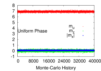
Figure 1: $\displaystyle m_{u},m_{z},m_{x}$ vs Monte Carlo history for $\displaystyle N=7$, $\displaystyle\mu=-35.1$, $\displaystyle c=0.36$, and $\displaystyle r=1$.

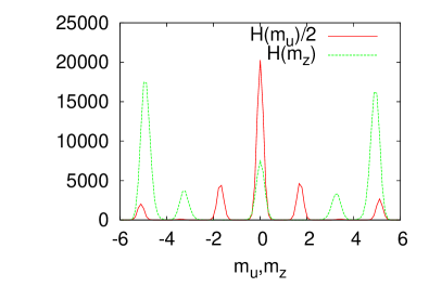
Figure 2: Histogram of $\displaystyle H(m_{u})$ and $\displaystyle H(m_{z})$ $\displaystyle N=7$, $\displaystyle\mu=-20.0$, $\displaystyle c=0.36$, and $\displaystyle r=1$.

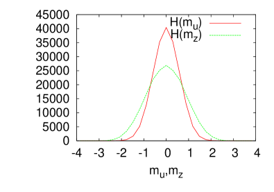
Figure 3: Histogram of $\displaystyle H(m_{u})$ and $\displaystyle H(m_{z})$ $\displaystyle N=7$, $\displaystyle c=0.36$, and $\displaystyle r=1$.

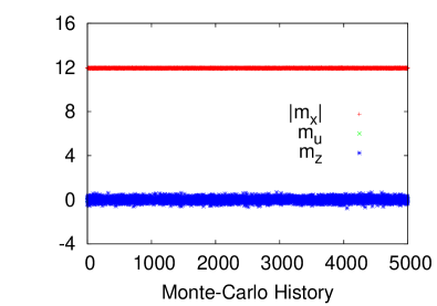
Figure 4: $\displaystyle m_{u},m_{z},m_{x}$ vs Monte Carlo history for $\displaystyle N=7$, $\displaystyle\mu=-3.6\times 10^{3}$, $\displaystyle c=36.$, $\displaystyle r=0.01$.

7 Conclusions

In this paper, we have considered a finite dimensional representation of the noncommutative cylinder algebra, which makes it fuzzy. We study scalar field theory in the background of this algebra both analytically and using numerical simulations.

The action of the scalar field on the fuzzy cylinder contains a kinetic as well as a potential term. The kinetic term leads to the Laplacian (28) on the fuzzy cylinder. We have analyzed the symmetries of the Laplacian and have obtained an algebraic equation (38,42) describing the corresponding spectrum.

In the numerical simulations of the scalar field with a generic potential we find, as expected in noncommutative theories, novel stripe phases breaking rotational symmetry. But they have some differences with the usual stripes on Moyal spacetimes. These are also stable due to topological features arising in this fuzzy geometry. A similar stability has been seen in the $\displaystyle O(3)$ model on fuzzy spheres digaltrg .

The fuzzy cylinder algebra considered in this paper is valid for non-extremal BTZ black holes, without any further assumptions. In addition, different forms of the BTZ metric related by coordinate transformations are equivalent classically, which at the algebraic level are expected to be related by automorphisms.

While the noncommutative cylinder algebra first arose in the context of the BTZ black hole, subsequently it has been shown to be of more general relevance, appearing in diverse backgrounds such as for Kerr black hole schupp and FRW cosmologies ohl . In addition, the near-horizon geometry of a large class of black holes contains an $\displaystyle AdS_{3}$ factor ooguri .

Thus, a large class of noncommutative black holes are described by a noncommutative cylinder algebra. The fuzzy cylinder algebra derived from it can therefore be used to define a fuzzy black hole. From general considerations dop2 , we know that such black holes can arise at the Planck scale. Our results provide a first glimpse about the phase structure of a quantum scalar field theory in the background of a fuzzy black hole at the Planck scale.

Acknowledgment This work was done as a part of the CEFIPRA/IFCPAR project 4004-1 entitled Fuzzy Approach to Quantum Field Theory and Gravity. The authors gratefully acknowledge the financial assistance from CEFIPRA/IFCPAR which was essential for this work.

References

- (1) S. Doplicher, K. Fredenhagen and J. E. Roberts, Commun. Math. Phys. 172 (1995) 187.
- (2) P. Aschieri, C. Blohmann, M. Dimitrijevic, F. Meyer, P. Schupp and J. Wess, Class. Quant. Grav. 22 (2005) 3511.
- (3) A.P. Balachandran, T.R. Govindarajan, K.S. Gupta, S. Kurkcuoglu, Class. Quant. Grav. 23 (2006) 5799.
- (4) B.P. Dolan, Kumar S. Gupta and A. Stern, Class. Quant. Grav. 24 (2007) 1647.
- (5) P. Schupp and S. Solodukhin, arXiv:0906.2724 [hep-th].
- (6) T. Ohl and A. Schenkel, JHEP 0910 (2009) 052.
- (7) M. Banados, C. Teitelboim and J. Zanelli, Phys. Rev. Lett. 69 (1992) 1849.
- (8) M. Banados, M. Henneaux, C. Teitelboim and J. Zanelli, Phys. Rev. D 48 (1993) 1506.
- (9) H. Grosse and P. Presnajder, Acta Phys. Slovaca 49 (1999) 185.
- (10) J. Lukierski, A. Nowicki, H. Ruegg and V. N. Tolstoy, Phys. Lett. B 264 (1991) 331.
- (11) J. Lukierski, H. Ruegg and W. J. Zakrzewski, Ann. Phys. 243 (1995) 90.
- (12) S. Meljanac and M. Stojić, Eur. Phys. J. C 47 (2006) 531.
- (13) S. Meljanac, A. Samsarov, M. Stojić and K. Gupta, Eur. Phys. J. C 53 (2008) 295.
- (14) M. Daszkiewicz, J. Lukierski and M. Woronowicz, J. Phys. A 42 (2009) 355201.
- (15) J. Lukierski, Rept. Math. Phys. 64 (2009) 299.
- (16) T. R. Govindarajan, K. S. Gupta, E. Harikumar, S. Meljanac and D. Meljanac, Phys. Rev. D 77 (2008) 105010.
- (17) T. R. Govindarajan, K. S. Gupta, E. Harikumar, S. Meljanac and D. Meljanac, Phys. Rev. D 80 (2009) 025014.
- (18) T.R.Govindarajan, Kumar S. Gupta, E. Harikumar and S. Meljanac, Journal of Physics: Conference Series 306 (2011) 012019.
- (19) Kumar S. Gupta, S. Meljanac and A. Samsarov, arXiv:1108.0341 [hep-th]
- (20) M. Chaichian, A. Demichev, P. Presnajder and A. Tureanu, Phys. Lett. B 515 (2001) 426.
- (21) A. P. Balachandran, T. R. Govindarajan, A. G. Martins and P. Teotonio-Sobrinho, JHEP 0411 (2004) 068.
- (22) J. Madore, An Introduction to Noncommutative Differential Geometry and its Physical Applications, (London Mathematical Society Lecture Note Series).
- (23) A.P. Balachandran, S. Kurkcuoglu and S. Vaidya, Lectures on fuzzy and fuzzy SUSY physics, World Scientific (2007).
- (24) J. Hoppe, Ph.D. Thesis, MIT (Cambridge MA, 1982).
-
(25)
A.P. Balachandran, T.R. Govindarajan and B. Ydri,
Mod. Phys. Lett. A15 (2000) 1279 [hep-th/9911087];
A.P. Balachandran, A. Pinzul and B.A. Qureshi, JHEP 0512 (2005) 002 [hep-th/0506037]. - (26) S.S. Gubser and S.L. Sondhi, Nucl. Phys. B605, 395 (2001) [hep-th/0006119].
- (27) X. Martin, JHEP 0404 (2004) 077 [hep-th/0402230].
-
(28)
J. Medina, W. Bietenholz, F. Hofheinz and
D. O’Connor, PoS LAT2005 (2005) 263 [hep-lat/0509162];
F. G. Flores, D. O’Connor and X. Martin, PoS LAT2005 (2006) 262 [hep-lat/0601012];
D. O’Connor and B. Ydri, JHEP 0611 (2006) 016 [hep-lat/0606013];
J. Medina, Phd. thesis, arXiv: 0801.1284 [hep-th]. -
(29)
W. Bietenholz, F. Hofheinz and J. Nishimura,
Acta. Phys. Polon. B34 (2003) 4711 [hep-th/0309216];
Nucl. Phys. Proc. Suppl. 129 (2004) 865 [hep-th/0309182]. -
(30)
M. Panero, SIGMA 2 (2006) 081 [hep-th/0609205];
JHEP 0705, 082 (2007) [hep-th/0608202]. - (31) C.R. Das, S. Digal and T.R. Govindarajan, Mod. Phys. Lett. A23 (2008) 1781.
- (32) C.R. Das, S. Digal and T.R. Govindarajan, Mod. Phys. Letts A24 (2009) 2693.
- (33) J. Ambjorn and S. Catterall, Phys. Lett. B549 (2002) 253 [hep-lat/0209106].
- (34) J. Medina, W. Bietenholz and D. O’Connor, JHEP 0804 (2008) 041 arXiv:0712.3366 [hep-th].
- (35) Denjoe O’Connor (private communication)
- (36) S. Digal and T. R. Govindarajan, arXiv:1108.3320 [hep-th]
- (37) O. Aharony, S. S. Gubser, J. M. Maldacena, H. Ooguri and Y. Oz, Phys. Rept. 323 (2000) 183 arXiv:hep-th/9905111.