$\mathcal{Z}$ Extremization in Chiral-Like Chern Simons Theories

Abstract

We study the localized free energy on $S^{3}$ of three-dimensional $\mathcal{N}=2$ Chern-Simons matter theories at weak coupling. We compute the two loop $R$ charge in three different ways, namely by the standard perturbative approach, by extremizing the localized partition function at finite $N$ and by applying the standard saddle point approximation for large $N$. We show that the latter approach does not reproduce the expected result when chiral theories are considered. We circumvent these problems by restoring a reflection symmetry on the eigenvalues in the free energy. Thanks to this symmetrization we find that the three methods employed agree. In particular we match the computation for a model whose four dimensional parent is the quiver gauge theory describing D$3$ branes probing the Hirzebruch surface. We conclude by commenting on the application of our results and to the strong coupling regime.

1 Introduction

Localization of three dimensional supersymmetric field theories on $S^{3}$ has recently attracted many investigations. Indeed it has been observed that it is not only an academic exercise, but this procedure offers a simple way to extract many information about SCFTs. The partition function and then the free energy computed by this procedure reduce to a matrix model which contains some quantum information once only the one loop determinants are evaluated. This technique, first applied to ${\cal N}\geq 3$ superconformal Chern Simons matter theories in Kapustin:2009kz , made it possible the computation of the large $N$ scaling of the free energy in $\mathcal{N}\geq 3$ theories Drukker:2010nc ; Herzog:2010hf , which are supposed to describe M$2$ branes probing a conical singularity which basis is a CY₄ Aharony:2008ug . This is a non trivial check of the conjectured duality because it was observed that the $N^{3/2}$ scaling of the free energy obtained from the supergravity side is recovered even by a direct computation in a strongly coupled field theory.

The ${\cal N}\geq 3$ partition function trivially depends on the $R$ charge of the matter fields, because the supersymmetry algebra implies that they keep their canonical dimensions also at the quantum level. A more complicated situation appears in the $\mathcal{N}=2$ case where the $R$ symmetry is abelian and it can mix with the other abelian symmetries of the theory. In this case the free energy is a function of the $R$ charge, and the properties of the $\mathcal{N}=2$ theories require the knowledge of the exact $R$ charge current appearing in the superconformal algebra. Surprisingly, as first observed in Jafferis:2010un , the exact $R$ charges have the special property of extremizing the free energy $\mathcal{F}$. In every known example this extremization is a maximization, and identifying the free energy as a good candidate for counting the number of degrees of freedom led to conjecture a three-dimensional c-theorem, known as ${\cal F}$-theorem Jafferis:2011zi ; Klebanov:2011gs ; Gulotta:2011si . In Klebanov:2011gs ; Amariti:2011xp , the $\mathcal{F}$-maximization was found to be valid along the whole RG flows of a large class of weakly coupled theories, even without supersymmetry Klebanov:2011gs , corroborating the validity of an $\mathcal{F}$-theorem. Other properties like the relation with the supergravity computations and the volumes of the $AdS$ dual geometry Martelli:2011qj ; Cheon:2011vi ; Jafferis:2011zi ; Fuji:2011km and the relation between the Lagrange multipliers enforcing the marginality of the superpotential terms and the coupling constants along the RG flows Amariti:2011xp were then observed.

In many classes of theories the $\mathcal{F}$ maximization procedure has been successfully applied and the known perturbative and non perturbative results Martelli:2011qj ; Cheon:2011vi ; Jafferis:2011zi ; Amariti:2011hw ; Niarchos:2011sn ; Minwalla ; Amariti:2011da ; Morita:2011cs have been recovered. Anyway there is a whole class of theories where the procedure has not been completely understood yet. This class is typical of theories with low supersymmetry ($\mathcal{N}=1$ in 4d and $\mathcal{N}=2$ in 3d) and consists of theories with a chiral like field content. In the language of quiver gauge theories they are represented as nodes (groups) connected by oriented edges (bi-fundamentals and adjoint fields), such that there are edges where the number of oriented arrows in one direction differs from the number of oriented arrows in the opposite direction. These theories are called chiral gauge theories. It was observed that at large $N$ and strong coupling ($N\gg k$) the free energy does not scale as $N^{3/2}$ as predicted by the conjectured supergravity dual and the $\mathcal{F}$ extremization procedure does not reproduce the volume computation. Understanding this mismatch is an open problem. Indeed if the large $N$ scaling is different from the one expected in supergravity these theories cannot describe the motion of M$2$ branes probing a toric CY₄. On the other hand if these theories provide the correct dual SCFT, then there must be subtleties in the large $N$ computation of the free energy.

The discussion above motivates the study of the free energy of theories with a chiral like field content. In this paper we discuss the large $N$ scaling limit of $\cal{F}$, but in the weakly coupled regime, where the CS level $k$ is larger than the gauge group rank $N$, and the ’t Hooft coupling $N/k$ is small. In this regime, the $R$ charges of the matter fields can be computed in several independent ways. We are interested in comparing the $\cal F$-extremization technique for large $k$ and finite $N$ as well as its large $k$, large $N$ saddle point approximation to the standard perturbative evaluation. We show that in the case of vector-like theories the three approaches give exactly the same result. Then we switch to a chiral theory with one gauge group with $N_{f}$ fundamental and $N_{\widetilde{f}}$ anti-fundamental with $N_{f}\neq N_{\widetilde{f}}$. In the latter theory we first compute the partition function for finite $N$ observing that the corresponding $R$ charge agrees with the expected one. Then we show that the naive saddle point equations at large $N$ do not reproduce the expected large $N$ result. We observe that, at this order, this is related to the explicit breaking of the reflection symmetry, on the large $N$ saddle point equations, acting on the eigenvalues of the Cartan subgroup of the gauge group. By restoring this symmetry, the $\mathcal{F}$-extremization procedure in its large $N$ saddle point approximation gives the same answer as the large $N$ limit obtained from the other two computations. We also check our proposal in the case of multiple gauge groups at the perturbative level by looking at a quiver gauge theory with the same field content and superpotential of the four dimensional $\mathbb{F}_{0}$ model but with a CS term for each gauge group and large levels $\{k_{i}\}$ (we refer to this theory as $\widetilde{\mathbb{F}_{0}}_{\{k_{i}\}}$). This theory in the strongly coupled regime is conjectured to describe M$2$ branes probing a CY₄ geometry (whose geometrical details depend from the choice of the CS levels). Moreover we observe that the Lagrange multiplier proposal of Amariti:2011xp can be extended to this chiral example straightforwardly. We finally consider a generalization of this theory to an arbitrary number of bi-fundamental fields and show that our method still gives the expected result.

The paper is organized as follows. In section 2 we review the basic aspects of the localized partition function and its relation with the exact $R$-charge. In section 3 we show the computation of the free energy at large $N$ but small ’t Hooft coupling. We discuss both vector like and chiral like examples, and observe that the latter cases match with the perturbative computation only after we restore the reflection symmetry on the Cartan subgroup. In section 4 we verify the Lagrange multiplier conjecture in the case of $\widetilde{\mathbb{F}_{0}}_{\{k_{i}\}}$. Then we conclude, and comment on some possible application of our method in the strongly coupled regime.

2 $\cal F$ extremization

As mentioned in the introduction, the localization technique has been shown to be a powerful tool to extract physical quantities in three-dimensional field theories. In the case of $\mathcal{N}\geq 3$ theories Kapustin:2009kz the $R$ symmetry is non abelian and the supersymmetry algebra constraints the matter fields to preserve their classical scaling dimension. In the $\mathcal{N}=2$ case, the classical value of the scaling dimension of the matter fields is not generically preserved along the RG flow. Indeed in this case the $R$-symmetry group $SO(2)_{R}\simeq U(1)_{R}$ is abelian and it can mix with all the other abelian flavor symmetries of the theory. Moreover it can also mix with topological symmetries related to the diagonal monopoles. The full localized partition function on $S^{3}$ is Jafferis:2010un ; Hama:2010av (up to an overall factor which is irrelevant for our purposes)

$$\mathcal{Z}_{S^{3}}=\int\text{d}[u]e^{i\pi k\text{Tr}u^{2}}{\det}_{\text{adj}}\sinh(\pi u)\prod_{\Phi}{\det}_{\rho_{R_{\Phi}}}e^{l\left(1-\Delta_{R_{\Phi}}+i\rho_{R_{\Phi}}(u)\right)}$$ (1)

The different contributions to this formula are

• The measure d$[u]$ is the measure over the Cartan of the gauge group. For example for a $U(N)$ model it is

  $$\text{d}[u]=\prod_{i=1}^{N}\text{d}u_{i}$$ (2)

• The exponential $e^{i\pi k\text{Tr}u^{2}}$ is the contribution coming from a CS term with level $k$. The trace is over the fundamental, namely Tr$u^{2}=u_{1}^{2}+\dots+u_{N}^{2}$ for the $U(N)$ case. The YM contribution vanishes because $g_{YM}$ is dimensionful in three dimensions.

• The determinant over the adjoint is the product of the roots and it comes from the one loop determinant of the vector field. In the $U(N)$ case it is explicitly

  $${\det}_{adj}\sinh\pi u=\prod_{i<j}\sinh^{2}(\pi(u_{i}-u_{j}))$$ (3)

• The last contribution is the one loop determinant of the matter fields. For every field $\Phi$ in the representation $R_{\Phi}$ of the gauge group the determinant is computed over the weights $\rho_{R_{\Phi}}$ of the representation. The function $l(z)$ has been found in Jafferis:2010un ; Hama:2010av after the zeta regularization of the otherwise divergent determinant. It is explicitly

  $$l(z)=-\frac{i\pi}{12}-z\,\text{Log}\left(1-e^{2i\pi z}\right)+\frac{1}{2}i\left(\pi z^{2}+\frac{\text{Li}_{2}\left(e^{2\pi iz}\right)}{\pi}\right)$$ (4)

  The partition function has an explicit dependence on the $R$ charge $\Delta$ through this function, which then represents the main difference with respect to the more supersymmetric models. Indeed when ${\cal N}\geq 3$ the non abelian nature of the $R$-symmetry group constraints $\Delta$ to acquire the classical value $1/2$ at the quantum level (no mixing is possible in this case) and the formula obtained in Kapustin:2009kz is recovered.

The proposal made in Jafferis:2010un consists of extracting the exact $R$ charge by extremizing the partition function (1) with respect to $\Delta$. Many examples were worked out both at strong and at weak coupling, comparing the results with the AdS/CFT predictions and the perturbative evaluations, respectively. In all the cases, the $\mathcal{Z}$-extremization reproduced the expected results.

A general strategy for computing the integral (1) is still lacking, but approximate computations of the free energy have been performed. For example at large $k$ Amariti:2011hw ; Amariti:2011da the saddle point contribution to the integral comes from $u_{i}\sim 0$, where the integrals reduce to simple gaussian integrals and the perturbative results are computed in terms of the small ’t Hooft coupling. Moreover in Minwalla the computation was simplified in the case of $k\gg N\gg 1$. In this case the saddle point equations can be solved perturbatively order by order in the eigenvalues. At the lowest order they obey a Wigner distribution and the classical $R$ charge is $R=1/2$. The solutions to the higher order equations are associated to the quantum corrections in the QFT perturbative expansion.

The strong coupling regime has been deeply investigated in Martelli:2011qj ; Jafferis:2011zi . The saddle point equations have been solved only for particular classes of theories, like the necklace non-chiral quiver gauge theories. These theories correspond to quiver gauge theories with bi-fundamentals connecting two adjacent groups, and a vector like field content. Indeed in this case it was shown that the eigenvalues at large $N$ scale as $u_{i}=\sqrt{N}x_{i}+iy_{i}$. This scaling and the structure of the quiver cancel the long range interactions among the eigenvalues and leave a local structure for the free energy. The $N^{3/2}$ scaling at large $N$ has been matched with the supergravity calculation and with the volume minimization. The validity of the $\mathcal{F}$-maximization has not been confirmed yet for the theories with a chiral like field content. The main obstruction is that in these cases the long range interactions among the eigenvalues cannot be cancelled as in the non-chiral cases, and the scaling of the free energy usually differs from the one expected by the supergravity computation.

Many interpretations are possible for this mismatch. It is possible that these theories do not describe the motion of M$2$ branes in the CY₄ geometry and cannot match with the AdS/CFT predictions. Another possibility is that there is some problem in the large $N$ approach. Motivated by this mismatch, in the rest of the paper we study the large $N$ saddle point equations for chiral like theories in the perturbative regime $k\gg N\gg 1$. We will show that a well defined large $N$ limit in this regime requires some care.

Weakly coupled theories have the advantage that we have many tools to carry out the computation, providing us with reliable checks about the validity of the results. Indeed, we will perform our computation in three different ways. First, we present the standard perturbative evaluation of Feynman diagrams. Secondly, we show that when we consider the finite $N$ partition function in the perturbative regime, we obtain the same results as the Feynman diagram evaluation. Finally, we show that in the large $N$ limit, namely in the saddle point approximation, some assumptions are breaking down, and we present a way to extract the right result. We show that our procedure works in several examples. Based on these results, we comment on the large $N$ limit in the strongly coupled regime.

3 Perturbative regime at large $k$ and $N$

Before we start our analysis a comment is in order. Even though in three dimensions there are no local gauge anomalies, the gauge invariance may require the introduction of a classical CS term which breaks parity Redlich:1983dv ; AlvarezGaume:1983ig . This is usually referred to as parity anomaly. For example in the abelian case with multiple $U(1)$’s there is a parity anomaly if

$$\frac{1}{2}\sum_{\text{fermions}}(q_{f})_{i}(q_{f})_{j}\in\mathbb{Z}+\frac{1}{2}$$ (5)

where $(q_{f})_{i}$ is the charge of the fermion $f$ under the $U(1)_{i}$. If it is the case a semi integer CS term must be added to restore parity. In the rest of the paper we restrict to the cases in which (5) is integer.

To the best of our knowledge the perturbative computations of the $R$ charges in the chiral theories the we are considering have never appeared in the literature. Anyway we will only present the final result and stress that it agrees with the other methods employed. The interested reader is referred to Avdeev:1992jt for the details of the standard perturbative approach.

In the rest of this section we will only consider $SU(N)$ models where it is possible to associate an $R$ charge to the fundamentals or bi-fundamentals. Anyway at large $N$ the difference between $U(N)$ and $SU(N)$ is sub-leading and we can trust in the extremization of the free energy associated to the $U(N)$ model. Indeed one can observe that at the order we are interested in the eigenvalues sum up to zero even in the $U(N)$ case, which corresponds to the $SU(N)$ traceless condition. In the Appendix A we explicitly observe the agreement at large $N$ of the $U(N)$ and $SU(N)$ computations.

3.1 $SU(N)_{k}$ with $N_{f}$ fundamentals and anti-fundamentals

We now apply the saddle point approximation to the weak coupling regime of a vector-like Chern-Simons theory. We couple the ${\cal N}=2$ vector supermultiplet $V$ to $N_{f}$(=$N_{\widetilde{f}}$) pairs $(\phi,\tilde{\phi})$ of fields in the (anti)fundamental representation of the gauge group $G=SU(N)_{k}$. For simplicity we consider a vanishing superpotential, but the extension to a more general case is straightforward.

The three-dimensional localized partition function for this model is

$$\mathcal{Z} = \int\prod_{i=1}^{N}du_{i}\text{Exp}\left(N^{2}\left(\frac{i\pi}{\lambda N}\sum_{i=1}^{N}u_{i}^{2}+\frac{1}{N^{2}}\sum_{i\neq j}\log\sinh\left(\pi u_{ij}\right)+\right.\right.$$ (6)

$$~{}~{}~{}~{}~{}~{}~{}~{}~{}~{}~{}~{}~{}~{}~{}~{}~{}~{}~{}~{}~{}~{}~{}~{}~{}~{}~{}~{}~{}~{}~{}~{}~{}~{}~{}~{}~{}~{}~{}~{}~{}+\left.\left.\frac{N_{f}}{N^{2}}\sum_{i;\eta=\pm 1}l(1-\Delta+i\eta u_{i})\right)\right)$$

where we defined the ’t Hooft coupling $\lambda\equiv N/k$. For large enough $N$, the main contribution to $\cal Z$ comes from the extremum of the argument of the exponential. In order to find the eigenvalues $\{u\}$ which correspond to this minimum, we write the following saddle point equations

$$\frac{i}{\lambda}u_{i}+\frac{1}{N}\sum_{j\neq i}\coth(\pi u_{ij})-\frac{iN_{f}}{2N}\sum_{\eta=\pm 1}\eta(1-\Delta+i\eta u_{i})\cot(1-\Delta+i\eta u_{i})=0$$ (7)

and we substitute the corresponding solution into the extremization equation for the $R$ charge

$$\text{Re}\left(\sum_{i;\eta=\pm 1}(1-\Delta+i\eta u_{i})\cot(\pi(1-\Delta+i\eta u_{i}))\right)=0$$ (8)

In the perturbative regime $\lambda\ll 1$ we expand the eigenvalues and the $R$ charge as Minwalla

$$\begin{split}u_{i}&=\sum_{n=0}^{\infty}u_{i}^{(n)}\lambda^{\frac{1}{2}+n}=\sqrt{\lambda}\left(u_{i}^{(0)}+\lambda u_{i}^{(1)}+\ldots\right)\\ \Delta&=\Delta^{(0)}+\lambda\Delta^{(1)}+\lambda^{2}\Delta^{(2)}+\ldots\end{split}$$ (9)

To lowest order, equation (8) sets $\Delta^{(0)}=1/2$, which is the classical scaling dimension, as expected in the perturbative case. By substitution in (7), we find that the $u_{i}^{(0)}$ satisfy

$$iu_{i}^{(0)}+\frac{1}{\pi N}\sum_{j(\neq i)}\frac{1}{u_{i}^{(0)}-u_{j}^{(0)}}=0$$ (10)

whose solution is known in the large $N$ limit: we rotate the eigenvalues according to $u_{i}^{(0)}=y_{i}\exp{(i\pi/4)}$ and because the variables $y_{i}$ become dense we substitute them with the continuos variable $y$. The eigenvalue distribution $\rho(y)$ has support on the interval $(-\sqrt{\frac{2}{\pi}},\sqrt{\frac{2}{\pi}})$ and takes the value

$$\rho(y)=\sum_{i=1}^{N}\delta(y-y_{i})=\sqrt{\frac{2}{\pi}-y^{2}}$$ (11)

Till now, we recovered the classical behavior of the field theory. The quantum corrections are contained in the higher order expansions of (7) and (8). In particular, one finds that the distribution $\rho(y)$ is not changed and as a consequence $\Delta^{(1)}=0$, again in agreement with perturbation theory.

We substitute back these results into (7) and expand till the next nontrivial order. After some manipulations we get the equation

$$\frac{1}{\pi N}\sum_{j\neq i}\frac{u_{j}^{(1)}}{u_{i}^{(0)}-u_{j}^{(0)}}=\frac{\pi}{6}\left(\frac{3N_{f}}{N}-2\right)u_{i}^{(0)}$$ (12)

We again rotate the variables in the complex plane as $u_{i}^{(0)}\rightarrow y_{i}=e^{-\frac{i\pi}{4}}u_{i}^{(0)}$ and $u_{i}^{(1)}\rightarrow v_{i}(y_{i})=e^{-\frac{i\pi}{4}}u_{i}^{(1)}$, and substitute the discrete $y_{i}$ and $v_{i}$ with the continuos variables $y$ and $v(y)$. Using the same technique explained in Minwalla we solve the corresponding equation obtaining

$$v(y)=-\frac{i\pi}{12}\left(\frac{3N_{f}}{N}-2\right)y$$ (13)

We now have all the necessary ingredients to compute the two-loop $R$ charge. Indeed, one first notes that at $\mathcal{O}(\lambda^{3/2})$ equation (8) is an identity, then one finds a nontrivial equation at $\mathcal{O}(\lambda^{2})$. Again, the latter can be solved by passing to the continuum limit which results in

$$\Delta=\frac{1}{2}-\lambda^{2}\frac{N_{f}}{2N}$$ (14)

Thus, we obtained the large $N$ limit of the full two-loop perturbative result Gaiotto:2007qi already computed for finite $N$ in Amariti:2011hw .

3.2 $SU(N)_{k}$ with different number of fundamentals and anti-fundamentals

3.2.1 Extremizing the finite $N$ partition function

For simplicity, we consider a ${\cal N}=2$ model with gauge group $SU(N)$ and $N_{f}$ massless chiral fields $\phi^{i}_{a}$, $a=1,\ldots,N$, $i=1,\ldots,N_{f}$ in the fundamental representation of the gauge group. The resulting partition function reads

$${\cal Z}=\int\prod_{i=1}^{N}du_{i}\text{Exp}\left(\!i\pi k\sum_{i=1}^{N}u_{i}^{2}+\sum_{i\neq j}\log\sinh\left(\pi u_{ij}\right)\!+\!\sum_{i}N_{f}l(1\!-\!\Delta\!+\!iu_{i})\!\!\right)\delta\!\left(\sum_{i=1}^{N}u_{i}\!\right)$$ (15)

By using the strategy of Marino:2002fk ; Aganagic:2002wv in the large $k$ limit, keeping $N$ fixed, (15) reduces to (up to an overall factor)

$$\begin{split}{\cal Z}&\simeq 1152k^{2}N(4+a^{2}N_{f}N\pi^{2})-(N^{2}-1)\pi^{2}(4(16N^{5}+9(1-4a)^{2}N_{f}^{2}N(N^{2}+1)+\\ &+12N_{f}(3+2N^{4}-8a(3-N^{2}+N^{4})))-a^{2}N_{f}(N(9NN_{f}^{2}(N^{2}+1)+\\ &+12N_{f}(3+6N^{2}-2N^{4})+16N(18-6N^{2}+N^{4}))-576)\pi^{2})+\\ &+48ikN(N^{2}-1)\pi(16N-N_{f}(12-a(48+a(4(N^{2}-3)-3N_{f}N)\pi^{2})))\end{split}$$ (16)

where $\Delta=1/2+a$. Upon extremization, we obtain the $R$ charge of the fields

$$\Delta=\frac{1}{2}-\frac{(NN_{f}-2)\left(N^{2}-1\right)}{4N^{2}k^{2}}$$ (17)

in full agreement with the perturbative result. We also performed a similar computation to extract the $R$ charge of a $SU(N)$ gauge theory coupled to $N_{f}$ fundamental fields $\phi_{a}^{i}$, $i=1,\ldots,N_{f}$ and $N_{\widetilde{f}}$ antifundamental fields $\tilde{\phi}_{i^{\prime}}^{a}$, $i^{\prime}=1,\ldots,N_{\widetilde{f}}$, with no superpotential term. The result, which again agrees with the perturbative one, is

$$\Delta_{1}=\Delta_{2}=\frac{1}{2}-\frac{\left(N\left(N_{f}+N_{\widetilde{f}}\right)-2\right)\left(N^{2}-1\right)}{4N^{2}k^{2}}$$ (18)

where $\Delta_{1}$ ($\Delta_{2}$) is the $R$ charge of $\phi$ ($\tilde{\phi}$).

This shows that, at least at weak coupling, the extremization procedure gives the correct exact $R$ charge. While we have no full reliable check of the validity of this statement either at higher orders in perturbation theory or at strong coupling, we do not see any obstruction for its validity.

3.2.2 The saddle point approach

We now apply to the $SU(N)$ gauge theory coupled to $N_{f}$ ($N_{\widetilde{f}}$) (anti)fundamental fields described at the end of the previous subsection the saddle point approximation, along the lines described in section 3.1. When the number of fundamentals and the number of anti-fundamentals do not coincide the partition function (6) becomes

$$\mathcal{Z} = \int\prod_{i=1}^{N}du_{i}\,\,\text{Exp}\left\{N^{2}\left(\frac{i\pi}{\lambda N}\sum_{i=1}^{N}u_{i}^{2}+\frac{1}{N^{2}}\sum_{i\neq j}\log\sinh\left(\pi u_{ij}\right)\right.\right.$$ (19)

$$+ \left.\left.\frac{1}{N^{2}}\sum_{i}N_{f}l(1-\Delta_{1}+iu_{i})+N_{\widetilde{f}}\,l(1-\Delta_{2}-iu_{i})\right)\right\}$$

As opposed to (6), the integrand of (19) is not invariant under the transformation $u_{i}\rightarrow-u_{i}$. While the latter ”parity” transformation is an obvious symmetry of the integrand of the partition function of all the vector-like three-dimensional models, such symmetry is explicitly broken in all the chiral models. As a result, we will now show that this makes the ansatz (9) inconsistent for the eigenvalues $\{u\}$.

Indeed, by solving order by order the saddle point equation

$$\frac{i}{\lambda}u_{i}+\frac{1}{N}\sum_{j\neq i}\coth(\pi u_{ij}) - \frac{iN_{f}}{2N}(1-\Delta+iu_{i})\cot(1-\Delta+iu_{i})+$$ (20)

$$- \frac{iN_{\widetilde{f}}}{2N}(1-\Delta-iu_{i})\cot(1-\Delta-iu_{i})=0$$

and the extremization equation, one finds that the solutions are the same as in the vector like case, but we also get two inconsistent equations. More precisely the saddle point equation (20) at order $\mathcal{O}(\lambda)$ gives ${u_{i}^{(0)}}^{2}=0$ which contradicts the ${\cal O}(\lambda^{-1/2})$ equation (10). This implies that some extra term has to be added in the expansion of the eigenvalues, such that the equation at this order can be solved. For example if the expansion is modified as

$$u_{i}=\sum_{n=0}^{\infty}u_{i}^{(n/2)}\lambda^{\frac{n+1}{2}}=\sqrt{\lambda}\left(u_{i}^{(0)}+\lambda^{1/2}u_{i}^{(1/2)}+\lambda u_{i}^{(1)}+\lambda^{3/2}u_{i}^{(3/2)}+\ldots\right)$$ (21)

then both the saddle point and the extremization equations can be consistently solved order by order in $\lambda$ up to the two-loop level. These require $u_{i}^{(1/2)}$ to vanish but $u_{i}^{(3/2)}$ not to vanish, while $u_{i}^{(0)}$ and $u_{i}^{(1)}$ obey equations analogous to those in section 3.1. Indeed in this case we can solve the equation at order $\mathcal{O}(\lambda)$ for $u_{i}^{(3/2)}$

$$iu_{i}^{(3/2)}+\frac{1}{\pi N}\sum_{j\neq i}\frac{u_{j}^{(3/2)}-u_{i}^{(3/2)}}{u_{j}^{(0)}-u_{i}^{(0)}}-i\pi\frac{N_{f}}{2N}{u_{i}^{(0)}}^{2}=0$$ (22)

which gives a non zero value for $u_{i}^{(3/2)}$. Despite this apparent success, we first note that the procedure just described seems model dependent and that it can still fail when different field content is considered. Secondly, and more important, the $R$ charge computed in this way does not match either with the perturbative computation or with the ${\cal Z}$-extremization result in section 3.2.1. This is a direct evidence that this approach does not allow to identify the saddle point that extremizes the partition function.

We now explain how to overcome this problem. We write the integrand of the partition function in a different way: the basic idea is that we want to make its integrand manifestly invariant under the parity symmetry $u_{i}\rightarrow-u_{i}$. Indeed, the measure

$$d\Gamma\left(\{u\}\right)\equiv\left(\prod_{i=1}^{N}du_{i}\right)\text{Exp}\left(N^{2}\left(\frac{i\pi}{\lambda N}\sum_{i=1}^{N}u_{i}^{2}+\frac{1}{N^{2}}\sum_{i\neq j}\log\sinh\left(\pi u_{ij}\right)\right)\right)$$ (23)

is invariant under parity, when one also considers that the domain of integration is the whole real axis. For vector-like theories, the matter contribution is also parity invariant. For chiral theories, this is no longer true, but we can write the partition function in the following way

$$\mathcal{Z} = \frac{1}{2}\int\prod_{i=1}^{N}du_{i}\text{Exp}\left(N^{2}\left(\frac{i\pi}{\lambda N}\sum_{i=1}^{N}u_{i}^{2}+\frac{1}{N^{2}}\sum_{i\neq j}\log\sinh\left(\pi u_{ij}\right)\right)\right)$$ (24)

$$\times \left\{\text{Exp}\left(\sum_{i}N_{f}l(1-\Delta_{1}+iu_{i})+N_{\widetilde{f}}l(1-\Delta_{2}-iu_{i})\right)\right.$$

$$\,\,+\left.\text{Exp}\left(\sum_{i}N_{\widetilde{f}}l(1-\Delta_{2}+iu_{i})+N_{f}l(1-\Delta_{1}-iu_{i})\right)\right\}$$

The partition function is exactly the same as the one in (19) but the symmetry $u_{i}\rightarrow-u_{i}$ is now manifest in $\mathcal{Z}$ and in the equations of motion. The latter are more involved than those derived from (19), but they are straightforward to write and solve order by order in $\lambda$. Moreover, the ansatz (9) turns out to be consistent at the two-loop level, that is, the solution to the saddle point equations and the partition function itself share some of the features of the vector-like models.

We computed the solutions both to the saddle point and to the extremization equations and found that the $R$ charge is

$$\Delta_{1}=\Delta_{2}=\frac{1}{2}-\lambda^{2}\frac{N_{f}+N_{\widetilde{f}}}{4N}$$ (25)

which agrees both with the large $N$ limit of (18) and, when $N_{f}=N_{\widetilde{f}}=N_{f}$, with (14).

A comment is in order. In the saddle point equations, the matter part of (24) contributes with a sum of terms. Each of them is weighted by a factor which reads (we set $N_{\tilde{f}}=0$ for simplicity, the generalization is straightforward)

$$\left(1+\exp\left\{N_{f}\sum_{i=1}^{N}\Big{[}l\left(1-\Delta_{1}+iu_{i}\right)-l\left(1-\Delta_{1}-iu_{i}\right)\Big{]}\right\}\right)^{-1}$$ (26)

Since the sum runs on $N$ terms of order ${\cal O}(1)$, in the large $N$ limit we expect the exponential to be either $1$, $0$ or divergent when evaluated on the solution for the $u_{i}$. If it is not $1$, the large $N$ and the ’t Hooft limit do not commute, as we cannot expand (26) in powers of $\lambda$. This would mean that our equations are being solved in an inconsistent way. If we assume that the eigenvalue distribution is parity invariant, that is, it satisfies $\sum_{i}\left(u_{i}^{(j)}\right)^{n}=0$ for odd $n$ but every $j$, the argument of the exponential in (26) vanishes. Because our solution satisfies this property, we conclude that the large $N$ and the ’t Hooft limit commute, and our result is fully consistent. A similar argument also holds when product gauge groups are considered.

We also checked, up to the order $\lambda^{5/2}$ in (21), that another sufficient condition for the exponential to be $1$ is that the $R$ charge in (26) is substituted with its perturbative value (25), without imposing any condition on the eigenvalue distribution.

3.3 A quiver field theory example: $\widetilde{\mathbb{F}}_{0}$

In this section we apply the result derived above to a more complicated example. This is a quiver gauge theory which in four dimensions represents the SCFT living on the world-volume of a stack of $N$ D$3$ branes probing a CY₃ conical singularity which has a base over the Hirzebruch surface or $\mathbb{F}_{0}$.

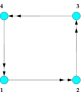
Figure 1: Quiver diagram for $\widetilde{\mathbb{F}}_{0}.$

The four-dimensional quiver gauge theory consists of a product of four $SU(N)$ gauge groups connected by chiral bi-fundamental fields as in Figure 1. The superpotential is

$$W=\epsilon_{ij}\epsilon_{kl}X_{12}^{(i)}X_{23}^{(l)}X_{34}^{(j)}X_{41}^{(k)}$$ (27)

In three dimensions at every gauge group is associated a CS term in the action with level $k_{i}$. At large $N$ it is conjectured to describe the dual field theory living on the world-volume of a stack of $N$ M$2$ branes probing a CY₄ conical singularity. The geometrical properties of the base of the cone are related to the value of the CS levels. For example in the case of $(k_{1},k_{2},k_{3},k_{4})=(k,k,-k,-k)$ this SCFT is conjectured to describe M$2$ branes probing a cone over $Q^{2,2,2}/\mathbb{Z}_{k}$. Anyway recently the mismatch in the large $N$ scaling of the free energy among the gravity dual and the field theory side placed an obstruction against this conjectured duality.

In the opposite regime $k\gg N\gg 1$ we observe a similar problem in the scaling of $\mathcal{F}$. In the case of a single gauge group we have been able to overcome the problem by restoring the symmetry $u\rightarrow-u$. Here we follow the same procedure for the $\widetilde{\mathbb{F}}_{0}$ theory, which original partition function is given by

$${\cal Z}=\int\left(\prod_{I=1}^{4}d\Gamma_{I}\right)f_{mat}\equiv\int\left[d\Gamma\right]f_{mat}$$ (28)

where we write $d\Gamma_{I}\equiv d\Gamma(\{u^{(I)}\})$ in equation (23) for brevity. Here, $f_{mat.}$ is the contribution of the matter fields, that in this case is

$$f_{mat.}=\text{Exp}\left(2\sum_{I=1}^{4}\sum_{i,j}l\left(1-\Delta_{I,I+1}+i(u_{i}^{(I)}-u_{j}^{(I+1)})\right)\right)$$ (29)

where the $I$s are identified mod $4$ and $\Delta_{I,I+1}$ is the $R$ charge of the fields which connect the $I$-th and the $(I+1)$-th node. We then symmetrize in analogy with the case with a single group obtaining

$$\mathcal{Z}=\frac{1}{2^{4}}\int[d\Gamma]g_{mat}$$ (30)

where the function $g_{mat}$ is

$$\sum_{Perm.\{\eta_{K}=\pm 1\}}\text{Exp}\left(2\sum_{I=1}^{4}\sum_{i,j}l\left(1-\Delta_{I,I+1}+i(\eta_{I}u_{i}^{(I)}-\eta_{I+1}u_{j}^{(I+1)})\right)\right)$$ (31)

where the sum is over all the possible $16$ permutations of the set $\{\eta_{K}\}$. We restored the full $\mathbb{Z}_{2}^{4}$ reflection symmetry, but up to the two loop order the same procedure also works if one only makes manifest the $\mathbb{Z}_{2}$ subgroup which acts by changing the sign of all the four groups of eigenvalues at once: $\left\{u_{I}\right\}\rightarrow-\left\{u_{I}\right\}$.

Now by making the ansatz (9) for the eigenvalues and the $R$ charges we can solve order by order the saddle point equations and compute the $R$ charges. Moreover in this case there is a constraint imposed by the superpotential

$$\sum_{I=1}^{4}\Delta_{I,I+1}=2$$ (32)

By applying the same technique as above, we get

$$\Delta_{12} = \frac{1}{2}-\frac{\lambda_{1}^{2}}{2}-\frac{3\lambda_{1}\lambda_{2}}{4}-\frac{\lambda_{2}^{2}}{2}+\frac{\lambda_{2}\lambda_{3}}{4}+\frac{\lambda_{3}^{2}}{2}+\frac{\lambda_{1}\lambda_{4}}{4}+\frac{\lambda_{3}\lambda_{4}}{4}+\frac{\lambda_{4}^{2}}{2}+\mathcal{O}(\lambda^{4})$$

$$\Delta_{23} = \frac{1}{2}+\frac{\lambda_{1}^{2}}{2}+\frac{\lambda_{1}\lambda_{2}}{4}-\frac{\lambda_{2}^{2}}{2}-\frac{3\lambda_{2}\lambda_{3}}{4}-\frac{\lambda_{3}^{2}}{2}+\frac{\lambda_{1}\lambda_{4}}{4}+\frac{\lambda_{3}\lambda_{4}}{4}+\frac{\lambda_{4}^{2}}{2}+\mathcal{O}(\lambda^{4})$$

$$\Delta_{34} = \frac{1}{2}+\frac{\lambda_{1}^{2}}{2}+\frac{\lambda_{1}\lambda_{2}}{4}+\frac{\lambda_{2}^{2}}{2}+\frac{\lambda_{2}\lambda_{3}}{4}-\frac{\lambda_{3}^{2}}{2}+\frac{\lambda_{1}\lambda_{4}}{4}-\frac{3\lambda_{3}\lambda_{4}}{4}-\frac{\lambda_{4}^{2}}{2}+\mathcal{O}(\lambda^{4})$$

$$\Delta_{41} = \frac{1}{2}-\frac{\lambda_{1}^{2}}{2}+\frac{\lambda_{1}\lambda_{2}}{4}+\frac{\lambda_{2}^{2}}{2}+\frac{\lambda_{2}\lambda_{3}}{4}+\frac{\lambda_{3}^{2}}{2}-\frac{3\lambda_{1}\lambda_{4}}{4}+\frac{\lambda_{3}\lambda_{4}}{4}-\frac{\lambda_{4}^{2}}{2}+\mathcal{O}(\lambda^{4})$$

in agreement with the field theory expectation, with $\lambda_{i}\equiv N/k_{i}$.

If we are not interested in an AdS/CFT example, we can consider the diagram of Figure 1 with an arbitrary number of bi-fundamental fields connecting each pair of nodes. If $\alpha_{I,I+1}$ is the number of fields connecting the $I$-th and the $(I+1)$-th node, with $\alpha_{I-1,I}=\alpha_{I,I+1}$ mod $2$ to avoid parity anomaly, our procedure gives the large $N$ result

$$\Delta_{12} = \frac{1}{2}-\frac{\lambda_{1}^{2}\alpha_{12}}{4}-\frac{3\lambda_{1}\lambda_{2}}{4}-\frac{\lambda_{2}^{2}\alpha_{23}}{4}+\frac{\lambda_{2}\lambda_{3}}{4}+\frac{\lambda_{3}^{2}\alpha_{34}}{4}+\frac{\lambda_{1}\lambda_{4}}{4}+\frac{\lambda_{3}\lambda_{4}}{4}+\frac{\lambda_{4}^{2}\alpha_{41}}{4}+\mathcal{O}(\lambda^{4})$$

$$\Delta_{23} = \frac{1}{2}+\frac{\lambda_{1}^{2}\alpha_{12}}{4}+\frac{\lambda_{1}\lambda_{2}}{4}-\frac{\lambda_{2}^{2}\alpha_{23}}{4}-\frac{3\lambda_{2}\lambda_{3}}{4}-\frac{\lambda_{3}^{2}\alpha_{34}}{4}+\frac{\lambda_{1}\lambda_{4}}{4}+\frac{\lambda_{3}\lambda_{4}}{4}+\frac{\lambda_{4}^{2}\alpha_{41}}{4}+\mathcal{O}(\lambda^{4})$$

$$\Delta_{34} = \frac{1}{2}+\frac{\lambda_{1}^{2}\alpha_{12}}{4}+\frac{\lambda_{1}\lambda_{2}}{4}+\frac{\lambda_{2}^{2}\alpha_{23}}{4}+\frac{\lambda_{2}\lambda_{3}}{4}-\frac{\lambda_{3}^{2}\alpha_{34}}{4}+\frac{\lambda_{1}\lambda_{4}}{4}-\frac{3\lambda_{3}\lambda_{4}}{4}-\frac{\lambda_{4}^{2}\alpha_{41}}{4}+\mathcal{O}(\lambda^{4})$$

$$\Delta_{41} = \frac{1}{2}-\frac{\lambda_{1}^{2}\alpha_{12}}{4}+\frac{\lambda_{1}\lambda_{2}}{4}+\frac{\lambda_{2}^{2}\alpha_{23}}{4}+\frac{\lambda_{2}\lambda_{3}}{4}+\frac{\lambda_{3}^{2}\alpha_{34}}{4}-\frac{3\lambda_{1}\lambda_{4}}{4}+\frac{\lambda_{3}\lambda_{4}}{4}-\frac{\lambda_{4}^{2}\alpha_{41}}{4}+\mathcal{O}(\lambda^{4})$$

which we matched with the two loop diagrammatic computation.

To conclude this section we observe that our discussion may be relevant at strong coupling, because the mismatch observed in Jafferis:2011zi with the expected AdS/CFT results should be ascribed to some problem in the identification of the saddle point, and the symmetrization of the integrand of $\mathcal{Z}$ may help in understanding the large $N$ scaling.

4 Lagrange multiplier

It is interesting to see whether the saddle point approximation can correctly describe the RG flow of the $R$ symmetry. As in Amariti:2011xp we here apply the technique of Kutasov:2003ux ; Kutasov:2004xu to answer this point.

For $\mathbb{F}_{0}$, we consider a modified version of the partition function of section 3.3

$$\widetilde{\cal Z}=\int[d\Gamma]\widetilde{f}_{mat.}$$ (35)

where $[d\Gamma]$ for this case is defined in section 3.3 and $\widetilde{f}_{mat}$ is

$$\widetilde{f}_{mat} = \text{Exp}\left(2\sum_{I=1}^{4}\sum_{i,j}l\left(1\!-\!\Delta_{I,I+1}\!+\!i(u_{i}^{(I)}\!-\!u_{j}^{(I+1)})\right)\!+\!m(\lambda_{1})\left(\sum_{I=1}^{4}\Delta_{I,I+1}-2\right)\right)$$

$$m(\lambda_{1}) = m_{0}+m_{2}\lambda_{1}^{2}$$ (36)

In the following discussion, $m(\lambda_{1})$ will play the role of a Lagrange multiplier which enforces the marginality constraint from the superpotential (27). A couple of comments are in order. We added only one Lagrange multiplier. As long as the number of bi-fundamental fields connecting two different nodes is the same this is perfectly consistent. Had we chosen a different number of fields connecting the different nodes, the renormalization group equations would have not preserved the whole symmetry of the superpotential (27) away from the fixed point, and we would have to add more multipliers. Secondly, we chose the Lagrange multiplier to be a function of $\lambda_{1}$ only. This is consistent because we are assuming that all the $\lambda$’s are small. Thus, we will write $\lambda_{i}=\lambda_{1}\frac{\lambda_{i}}{\lambda_{1}}$ and we will expand our saddle point equations in powers of $\lambda_{1}$. As long as $\lambda_{i}\ll 1$, $i=1,\ldots,4$ this gives the right result.

We symmetrize the first term in $\widetilde{f}_{mat}$ as discussed in the previous sections, and derive the saddle point equations which are not affected by the Lagrange multiplier. Then, we write the four extremization equations which simply reads

$$\frac{\partial}{\partial\,\Delta_{I,I+1}}\,\log{\widetilde{f}_{mat}}=0\qquad I=1,\ldots,4$$ (37)

and compute the solution as a function of $m(\lambda_{1})$. At the fixed point, after we substituted back into the partition function the solution to (37), the equation

$$\frac{\partial}{\partial\,m(\lambda_{1})}\,\log{\widetilde{f}_{mat}}=0$$ (38)

also holds. It is the latter equation which enforces the marginality of the superpotential; once it is imposed, it allows us to find the fixed point superpotential coupling $h$, which is related to $m$, as a function of the fixed point ’t Hooft couplings $\lambda$’s.

We do not discuss the solution in details, as the procedure used and the solution itself are very similar to those in section 3.3. Thus, we only present the results, mentioning that the equations set $m_{0}=0$ and

$$\Delta_{12} = \frac{1}{2}-\lambda_{1}^{2}-\lambda_{1}\lambda_{2}-\lambda_{2}^{2}-\frac{m_{2}\lambda_{1}^{2}}{\pi^{2}}+\mathcal{O}(\lambda^{4})$$

$$\Delta_{23} = \frac{1}{2}-\lambda_{2}^{2}-\lambda_{2}\lambda_{3}-\lambda_{3}^{2}-\frac{m_{2}\lambda_{1}^{2}}{\pi^{2}}+\mathcal{O}(\lambda^{4})$$

$$\Delta_{34} = \frac{1}{2}-\lambda_{3}^{2}-\lambda_{3}\lambda_{4}-\lambda_{4}^{2}-\frac{m_{2}\lambda_{1}^{2}}{\pi^{2}}+\mathcal{O}(\lambda^{4})$$

$$\Delta_{41} = \frac{1}{2}-\lambda_{1}^{2}-\lambda_{1}\lambda_{4}-\lambda_{4}^{2}-\frac{m_{2}\lambda_{1}^{2}}{\pi^{2}}+\mathcal{O}(\lambda^{4})$$

By comparison with the perturbative result (LABEL:eq:RF0), we obtain

$$m_{2}\lambda_{1}^{2}=\frac{|h|^{2}N^{2}}{16}$$ (40)

which is the expected relation from the discussion in Amariti:2011xp .

5 Discussion

In this paper we have studied the large $N$ behavior of the free energy at the perturbative level for both vector and chiral like gauge theories. We carried out the analysis by solving the saddle point equations for the eigenvalues with an appropriate ansatz. We observed that in the non-chiral case this procedure reproduces the two loop calculations, while in the case of theories with a chiral matter content the saddle point equations cannot be solved order by order in the ’t Hoof coupling. We have shown that this problem can be overcome by restoring the Weyl symmetry over the Cartan of every gauge group on the saddle point equation. This symmetrization acts on the integrand but it does not modify the free energy, which is indeed integrated over the Cartan subgroup. We have shown that after this transformation, a convenient ansatz correctly solves the equations at least at the lowest order in the ’t Hooft coupling, and by extremizing the free energy around the saddle point the two loop field theory results have been reproduced.

It would be important to go beyond the two loop approximation and observe whether the procedure that we have worked out in this paper does still apply. There are two interesting checks. The first consists of matching the $\lambda^{4}$ order which can be obtained with our procedure with the direct computation of the partition function at large $k$ but finite $N$, where the large $N$ limit can be safely taken after the integration over the variables $u$. This is just a consistency check for the computation of the partition function. A more complete check consists of matching with the four loop perturbation theory.

As already observed in the introduction this paper does not address the problem of the large $N$ behavior of chiral like gauge theories at strong coupling. In many cases the expected result can be computed from the AdS/CFT correspondence. Indeed if a chiral gauge theory describes the motion of M$2$ branes probing a toric CY₄ cone over a Sasaki Einstein manifold Y, then the free energy is related to the volume of Y. Recently in Gulotta:2011aa it has been observed that the computation of the volumes matches with the counting of the number of gauge invariant operators with a given $R$ and monopole charge.

This procedure was also applied to the $M^{1,1,1}/\mathbb{Z}_{k}$ case, and it was observed that this counting matches with the geometrical computation of the volumes as a function of the trial $R$ charges. Anyway this counting does not match with the eigenvalues distribution obtained from the saddle point equations of the free energy in the chiral cases. It would be worth to obtain the $N^{3/2}$ scaling of the free energy and the matching among the field theory and the supergravity computation from a purely field theoretical extremization of $\mathcal{F}$ and see whether the conjecture above holds. We think that our procedure can give some hints to study this problem. Indeed our main result consists in rewriting the partition function such that some symmetries become explicit in the saddle point equations. These restored symmetries then allow to maintain the same ansatz conjectured for vector like theories also in the chiral case. It is possible that also at strong coupling a similar procedure would allow for a consistent solution of the saddle point equations in terms of the common ansatz $u_{i}=\sqrt{N}x_{i}+iy_{i}$ , which leads to the expected result ${\cal F}\propto N^{3/2}$.

Appendix A Monopoles

Let us consider the partition function for a ${\cal N}=2$ Chern-Simons theory coupled to $N_{f}$ fundamental fields

$${\cal Z}=\int\!\!\prod_{i}du_{i}\,\,e^{ik\pi\sum_{i}u_{i}^{2}}\,e^{-\Delta_{m}\sum_{i}u_{i}}\,\prod_{i<j}\sinh^{2}\left(\pi u_{ij}\right)\,e^{N_{f}\sum_{i}l\left(1-\Delta+iu_{i}\right)}$$ (41)

We write the argument of the CS and monopole contributions as

$$ik\pi\left(u_{i}^{2}+i\frac{\Delta_{m}u_{i}}{k\pi}\right)=ik\pi\left(u_{i}+i\frac{\Delta_{m}}{2\pi k}\right)^{2}+i\frac{\Delta_{m}^{2}}{4\pi k}$$ (42)

We shift the integration variables as

$$u_{i}=u_{i}^{\prime}-i\frac{\Delta_{m}}{2\pi k}$$ (43)

and we substitute (42) and (43) into (41)

$${\cal Z}=e^{i\frac{\Delta_{m}^{2}}{4\pi k}}\int\!\!\prod_{i}du_{i}\,\,e^{ik\pi\sum_{i}u_{i}^{2}}\,\prod_{i<j}\sinh^{2}\left(\pi u_{ij}\right)\,e^{N_{f}\sum_{i}l\left(1-\Delta+\frac{\Delta_{m}}{2\pi k}+iu_{i}\right)}$$ (44)

The last formula makes two things manifest. First, the charges only appear in the combination $\Delta-\frac{\Delta_{m}}{2\pi k}$. When the gauge group is $U(N)$, we can impose $\sum_{SU(N)}u_{i}=0$ so that only the $U(1)$ weight in (43) is shifted. Then, $\Delta_{m}$ in (44) only appears in the $U(1)$ contribution. This corresponds to the fact that gauging a $U(1)$ symmetry one introduces a gauge field which couples to $j_{matter}+kj_{top}$. Secondly, in the perturbative regime $k\gg 1$, the monopole contribution is suppressed by a factor $1/k$ with respect to the contribution from the $R$ charge $\Delta$. Thus, at least up to the two loop order, the monopole charge vanishes, and the difference between the $SU(N)$ and the $U(N)$ theories is only due to the different values of the Casimir operators. In the large $N$ limit this difference is subleading in $N$ and the two models coincide, as expected from standard perturbation theory.

References

- (1) A. Kapustin, B. Willett, and I. Yaakov, Exact Results for Wilson Loops in Superconformal Chern- Simons Theories with Matter, JHEP 03 (2010) 089, [arXiv:0909.4559].
- (2) N. Drukker, M. Marino, and P. Putrov, From weak to strong coupling in ABJM theory, Commun.Math.Phys. 306 (2011) 511–563, [arXiv:1007.3837].
- (3) C. P. Herzog, I. R. Klebanov, S. S. Pufu, and T. Tesileanu, Multi-Matrix Models and Tri-Sasaki Einstein Spaces, Phys.Rev. D83 (2011) 046001, [arXiv:1011.5487].
- (4) O. Aharony, O. Bergman, D. L. Jafferis, and J. Maldacena, N=6 superconformal Chern-Simons-matter theories, M2-branes and their gravity duals, JHEP 0810 (2008) 091, [arXiv:0806.1218].
- (5) D. L. Jafferis, The Exact Superconformal R-Symmetry Extremizes Z, arXiv:1012.3210.
- (6) G. Festuccia and N. Seiberg, Rigid Supersymmetric Theories in Curved Superspace, JHEP 1106 (2011) 114, [arXiv:1105.0689].
- (7) D. L. Jafferis, I. R. Klebanov, S. S. Pufu, and B. R. Safdi, Towards the F-Theorem: N=2 Field Theories on the Three-Sphere, JHEP 1106 (2011) 102, [arXiv:1103.1181].
- (8) I. R. Klebanov, S. S. Pufu, and B. R. Safdi, F-Theorem without Supersymmetry, arXiv:1105.4598.
- (9) D. R. Gulotta, C. P. Herzog, and S. S. Pufu, From Necklace Quivers to the F-theorem, Operator Counting, and T(U(N)), arXiv:1105.2817.
- (10) A. Amariti and M. Siani, F-maximization along the RG flows: A Proposal, arXiv:1105.3979.
- (11) D. Martelli and J. Sparks, The large N limit of quiver matrix models and Sasaki-Einstein manifolds, Phys.Rev. D84 (2011) 046008, [arXiv:1102.5289].
- (12) S. Cheon, H. Kim, and N. Kim, Calculating the partition function of N=2 Gauge theories on and AdS/CFT correspondence, JHEP 1105 (2011) 134, [arXiv:1102.5565]. * Temporary entry *.
- (13) H. Fuji, S. Hirano, and S. Moriyama, Summing Up All Genus Free Energy of ABJM Matrix Model, JHEP 1108 (2011) 001, [arXiv:1106.4631].
- (14) A. Amariti, On the exact R charge for N=2 CS theories, JHEP 06 (2011) 110, [arXiv:1103.1618].
- (15) V. Niarchos, Comments on F-maximization and R-symmetry in 3D SCFTs, J.Phys.A A44 (2011) 305404, [arXiv:1103.5909]. * Temporary entry *.
- (16) S. Minwalla, P. Narayan, T. Sharma, V. Umesh, and X. Yin, Supersymmetric States in Large N Chern-Simons-Matter Theories, arXiv:1104.0680.
- (17) A. Amariti and M. Siani, Z-extremization and F-theorem in Chern-Simons matter theories, arXiv:1105.0933.
- (18) T. Morita and V. Niarchos, F-theorem, duality and SUSY breaking in one-adjoint Chern-Simons-Matter theories, arXiv:1108.4963. * Temporary entry *.
- (19) N. Hama, K. Hosomichi, and S. Lee, Notes on SUSY Gauge Theories on Three-Sphere, JHEP 1103 (2011) 127, [arXiv:1012.3512].
- (20) T. Suyama, Eigenvalue Distributions in Matrix Models for Chern-Simons-matter Theories, arXiv:1106.3147.
- (21) F. Benini, C. Closset, and S. Cremonesi, Chiral flavors and M2-branes at toric CY4 singularities, JHEP 02 (2010) 036, [arXiv:0911.4127].
- (22) D. L. Jafferis, Quantum corrections to N=2 Chern-Simons theories with flavor and their AdS4 duals, arXiv:0911.4324.
- (23) A. Redlich, Parity Violation and Gauge Noninvariance of the Effective Gauge Field Action in Three-Dimensions, Phys.Rev. D29 (1984) 2366–2374.
- (24) L. Alvarez-Gaume and E. Witten, Gravitational Anomalies, Nucl.Phys. B234 (1984) 269.
- (25) L. Avdeev, D. Kazakov, and I. Kondrashuk, Renormalizations in supersymmetric and nonsupersymmetric nonAbelian Chern-Simons field theories with matter, Nucl.Phys. B391 (1993) 333–357.
- (26) D. Gaiotto and X. Yin, Notes on superconformal Chern-Simons-Matter theories, JHEP 0708 (2007) 056, [arXiv:0704.3740].
- (27) M. Marino, Chern-Simons theory, matrix integrals, and perturbative three manifold invariants, Commun.Math.Phys. 253 (2004) 25–49, [hep-th/0207096].
- (28) M. Aganagic, A. Klemm, M. Marino, and C. Vafa, Matrix model as a mirror of Chern-Simons theory, JHEP 0402 (2004) 010, [hep-th/0211098].
- (29) N. Akerblom, C. Saemann, and M. Wolf, Marginal Deformations and 3-Algebra Structures, Nucl.Phys. B826 (2010) 456–489, [arXiv:0906.1705].
- (30) M. S. Bianchi, S. Penati, and M. Siani, Infrared stability of ABJ-like theories, JHEP 1001 (2010) 080, [arXiv:0910.5200].
- (31) M. S. Bianchi, S. Penati, and M. Siani, Infrared Stability of N = 2 Chern-Simons Matter Theories, JHEP 1005 (2010) 106, [arXiv:0912.4282].
- (32) D. Kutasov, New results on the ’a-theorem’ in four dimensional supersymmetric field theory, hep-th/0312098.
- (33) D. Kutasov and A. Schwimmer, Lagrange multipliers and couplings in supersymmetric field theory, Nucl.Phys. B702 (2004) 369–379, [hep-th/0409029].
- (34) D. R. Gulotta, C. P. Herzog, and S. S. Pufu, Operator Counting and Eigenvalue Distributions for 3D Supersymmetric Gauge Theories, arXiv:1106.5484.