On the active manipulation of quasistatic fields and its applications

Abstract

Following the ideas proposed in [10] and [11] on active exterior cloaking, we present here a systematic integral equation method to generate suitable quasistatic fields for cloaking, illusions and energy focusing (with given accuracy) in multiple regions of interests. In the quasistatic regime, the central issue is to design appropriate source functions for the Laplace equation so that the resulting solution will satisfy the required properties. We show the existence and non-uniqueness of solutions to the problem and study the physically relevant unique $L^{2}$-minimal energy solution. we also provide some numerical evidences on the feasibility of the proposed approach.

Key words. Field manipulation, quasistatics, layer potentials, integral equation, minimal energy solution, active exterior cloaking.

1 Introduction

The technique of manipulating acoustic and electromagnetic fields in desired regions of space has been greatly advanced in the recent years, mainly due to its fascinating applications such as, cloaking, the creation of illusions, secret remote communication, focusing energy, and novel imaging techniques. The development can be roughly classified into two categories.

The first type of techniques attempts to passively control the fields in the regions of interest by changing the material properties of the medium in certain surrounding regions while the second type of schemes focus on the active manipulation (active control) of fields with the help of specially designed sources.

In [8] the authors presented the first rigorous discussion of the passive manipulation of fields in the context of quasistatics cloaking (see also [29], [30] and [31] where the invariance to a change of variables is fully explained and the transformed material are fully described), and was later extended in [23] to the general case of passive manipulation of fields in the finite frequency regime (see also the review [4] and references therein). These passive strategies are now known as “transformation optics”. The similar strategy in context of acoustics was proposed in [6] (see also the review [3] and references therein). The idea behind transformation optics/acoustics is the invariance of the corresponding Dirichlet to Neumann-map (boundary measurements map) considered on some external boundary with respect to suitable change of variables which are identity on the respective boundary. This result implies that two different materials (the initial one and the one obtained after the change of variables is applied) occupying some region of space $\Omega$, will have the same boundary measurements maps on $\partial\Omega$ and thus be equivalent from the point of view of an external observer. This leads to a long list of important applications, such as, cloaking, field concentrators ([36]) or field rotators, illusion optics, etc. (see [4], [3], [7], [1] and references therein), cloaking sensors while maintaining their sensing capability [46], [47],

Recently, in an effort to improve accuracy and stability of the transformation optics/acoustics, various regularization of this scheme have been studied (see [14] and references therein, [26], [25], [28], [34], [32], [33]). Positive results about generating broadband low-loss metamaterial response have been obtained in [24], [35] and a new, more stable regularization strategy was recently proposed in [27].

In a parallel direction, many researchers focused on other alternative field manipulation strategies. They can be grouped into two main categories, passive designs based either on artificial materials with extreme properties or on geometrical arguments, and active designs based on the active control of fields by only using antennas with no materials needed in the scheme,

Among the alternative passive techniques proposed in the literature we could mention, plasmonic designs (see [1] and references therein), strategies based on anomalous resonance phenomena (see [20], [22], [21]), conformal mapping techniques (see [18],[17]), and complimentary media strategies (see [16]).

Regarding the active designs for the manipulation of fields we mention that this idea appeared first in the context of low-frequency acoustics where various techniques for the active control of low-frequency sound (or active noise cancellation) were proposed in the literature, and we could mention here the pioneer works of Leug [44] (feedforward control of sound) and Olson & May [45] (feedback control of sound). For a more detailed account of very interesting recent developments of the idea in the context of acoustics we mention the reviews [40], [42], [43], [38] [39] and the references therein.

In the electromagnetic regime, several active designs have been recently proposed in the literature and we could mention the interior active cloaking strategy proposed in [19] which uses active boundaries and the exterior active cloaking scheme discussed in [10], [11], [12], [9] (see also [48]) which uses a discrete number of active sources (antennas) to manipulate the fields. The active exterior strategy for 2D quasistatics cloaking was introduced in [10], were based on a priori information about the incoming field, with the help of one active source (antenna), we constructively described how one can create an almost zero field external region while maintaining a very small scattering effect in the far field. The proposed strategy did not work for objects closed to the antennas, it cloaked large objects only when they are far enough to the antenna (see [9]) and was not adaptable for three space dimensions. The finite frequency case was studied in the last section of [10] and in [12] (see also [9] for a recent review) where three active sources (antennas) were needed to create a zero field region in the interior of their convex hull while creating a very small scattering effect in the far field. The broadband character of the proposed scheme was numerically observed in [11]. We mention now that, from the point of view of the possible applications the constraint that the antennas surround the region of interests is not desirable and one would like to find a solution for the active manipulation of fields by using only one active source (antenna) as we proposed in [10].

In this paper, we address the problem formulated in Question 1 for the particular case of the quasistatic regime and a homogeneous environment). This problem is of course ill-posed and this explains the multitude of possible approximate solutions proposed for it. Our aim is to provide a unified mathematical theory for the general problem of active manipulation of electromagnetic or acoustic fields, which will work in a broadband regime and regardless of dimension, will allow for robust computational simulations and for the approximation of a stable optimal energy solution and will be appropriate for the more general case of non-homogeneous environments. In the present work we introduce the mathematical theory and analyse the problem in the quasistatic regime (modelled by the Laplace operator) corresponding to a homogeneous environment.

The paper is organized as follows. In Section 2 we formulate mathematically the problem of generating desired field in certain regions of space using active sources. We then study in Section 3 the existence of solutions of the mathematical problem and Section 4 the the constructive approximation of a solution with minimum energy. We provide some numerical simulations to support our theoretical results in Section 5. Concluding and further remarks are offered in Section 6. Finally, for the sake of completeness, we added the proofs for two technical results in the Appendix.

2 Problem formulation

Let $D_{\delta}\subset{\mathbb{R}}^{d}$ ($d=2,3$) be a small neighborhood of the origin ${\bf 0}$, and $D$ a given smooth domain containing $D_{\delta}$. Let the regions of interest, $\{D_{k}\}_{k=1}^{N}$, be $N$ subdomains of $D$ (i.e. $D_{k}\subset\subset D$, $1\leq k\leq N$) that are disjoint in the sense that $\overline{D}_{k}\cap\overline{D}_{k^{\prime}}=\emptyset,\forall k\neq k^{\prime}$. We also require that $D_{\delta}$ be disjoint with $D_{k}$, $\overline{D}_{\delta}\cap\overline{D}_{k}=\emptyset,\mbox{ for all }k$. We denote $u_{0}$ a smooth function on ${\mathbb{R}}^{d}\backslash\overline{D}$, and by $u_{k}$ a smooth function that is harmonic in a neighborhood of $D_{k}$, i.e. $\Delta u_{k}=0$ in $V\subset{\mathbb{R}}^{d}$ with $D_{k}\subset\subset V$. Then the general mathematical question that we want to ask in quasistatic regime is:

Question 1.

Can we design an exterior active source (antenna), modeled as a continuous function $h({\bf x})$ supported on $\partial D_{\delta}$, such that the harmonic field in ${\mathbb{R}}^{d}\backslash D_{\delta}$ generated by $h({\bf x})$, say $u$, has the property that $u\approx u_{0}$ in ${\mathbb{R}}\backslash\overline{D}$ and $u\approx u_{k}$ in $D_{k}$ for all $1\leq k\leq N$, where by $\approx$ we mean a good approximation in the uniform convergence norm?

This question appears naturally in many applications. For instance, if the answer to Question 1 is positive, then one can use the active source (antenna) on $D_{\delta}$ to generate a zero field in $\bigcup_{k=1}^{N}D_{k}$ and a scattering field $u_{0}$ corresponding to an arbitrary object in ${\mathbb{R}}^{d}\backslash\overline{D}$ to create an illusion for an external (outside of $\overline{D}$) observer. One can also program the active source (antenna) to approximate $N$ different desired fields in each of the regions $D_{k}$, $1\leq k\leq N$ while creating a zero field region in ${\mathbb{R}}^{d}\backslash\overline{D}$, thus sending information to regions of interests without being detected by an outside observer.

We now study Question 1 in more detail. To simplify the presentation, but without loss of generality, we assume that all regions involved in Question 1 are balls in ${\mathbb{R}}^{d}$. We denote by $B_{r}({\bf x})$ the d-dimensional open ball that centered at ${\bf x}\in{\mathbb{R}}^{d}$ with radius $r>0$. Moreover, we first present the case where only one region of interests is involved and then, in Remark 4.1, show how the general result (i.e., the case of $N$ region of interests) follows as an immediate consequence. Thus, let us consider Question 1 with $N=1$, $D_{\delta}=B_{\delta}(0)$, $D=B_{R}({\bf 0})$ and $D_{1}=B_{a}({\bf x}_{0})$ and (for technical reasons to be discussed later) new parameters $R^{\prime}$, and $a^{\prime}$ such that

$$a<a^{\prime},\ R^{\prime}<R,\ |{\bf x}_{0}|>a^{\prime}+\delta,\ \mbox{ and }\ R^{\prime}>|{\bf x}_{0}|+a^{\prime}.$$ (2.1)

A schematic illustration of the problem setting and various geometrical parameters are show in Fig. 1. Then, in the case when $u_{0}$ denotes a homogeneous quasistatic potential Question 1 can be formulated mathematically as follows.

Formulation A.

Let $0<\varepsilon\ll 1$ be fixed. Find a function $h\in C(\partial B_{\delta}({\bf 0}))$ such that there exists $v\in C^{2}({\mathbb{R}}^{d}\setminus\overline{B}_{\delta}({\bf 0}))\cap C^{1}({\mathbb{R}}^{d}\setminus B_{\delta}({\bf 0}))$ solution of,

$$\vspace{0.15cm}\left\{\vspace{0.15cm}\begin{array}[]{llll}\Delta v=0\mbox{ in }{\mathbb{R}}^{d}\setminus\overline{B}_{\delta}({\bf 0})\vspace{0.15cm}\\ v=h\mbox{ on }\partial B_{\delta}({\bf 0})\vspace{0.15cm}\\ \|v-u_{1}\|_{C(\bar{B}_{a}({\bf x}_{0}))}\leq\varepsilon\vspace{0.15cm}\\ \|v-u_{0}\|_{C({\mathbb{R}}^{d}\setminus B_{R}({\bf 0}))}\leq\varepsilon\end{array}\right.$$ (2.2)

where $u_{1}$ is a given function harmonic in a set containing $B_{a}({\bf x}_{0})$ and the norm $\|\cdot\|_{C(X)}$ is the usual uniform norm on continuous functions defined on $X$.

Figure 1: The geometrical setting of Formulation A.

If we subtract $u_{0}$ from $v$ in Formulation A, and denote by $u\equiv v-u_{0}$, $g\equiv h-u_{0}$, we obtain an equivalent formulation of the original problem.

Formulation A^′.

Let $0<\varepsilon\ll 1$ be fixed. Find a function $g\in C(\partial B_{\delta}({\bf 0}))$ such that there exists $u\in C^{2}({\mathbb{R}}^{d}\setminus\overline{B}_{\delta}({\bf 0}))\cap C^{1}({\mathbb{R}}^{d}\setminus B_{\delta}({\bf 0}))$ solution of,

$$\vspace{0.15cm}\left\{\vspace{0.15cm}\begin{array}[]{llll}\Delta u=0\mbox{ in }{\mathbb{R}}^{d}\setminus\overline{B}_{\delta}({\bf 0})\vspace{0.15cm}\\ u=g\mbox{ on }\partial B_{\delta}({\bf 0})\vspace{0.15cm}\\ \|u+u_{0}-u_{1}\|_{C(\bar{B}_{a}({\bf x}_{0}))}\leq\varepsilon\vspace{0.15cm}\\ \|u\|_{C({\mathbb{R}}^{d}\setminus B_{R}({\bf 0}))}\leq\varepsilon\end{array}\right.$$ (2.3)

Thus a solution of our problem is a function $g\in C(\partial B_{\delta})$ (resp. $h\in C(\partial B_{\delta})$ for (2.2)), such that there exists at least a solution for problem (2.3) (resp. (2.2)). Such a solution will describe the required potential to be generated at the active source (antenna) so that an approximation of $0$ (resp. $-u_{0}$) in the region $B_{a}({\bf x}_{0})$ with $\varepsilon$-accuracy will be possible with a very small perturbation of the far field (resp. very small far field).

Let $a^{\prime},R^{\prime},{\bf x}_{0},\delta$ be as before. We introduce the following space $\Xi$,

$$\Xi\equiv L^{2}(\partial B_{a^{\prime}}({\bf x}_{0}))\times L^{2}(\partial B_{R^{\prime}({\bf 0})})$$ (2.4)

Then $\Xi$ is a Hilbert space with respect to the scalar product given by

$$(\varphi,\psi)_{\Xi}=\int_{\partial B_{a^{\prime}}({\bf x}_{0})}\varphi_{1}({\bf y})\psi_{1}({\bf y})ds_{{\bf y}}+\int_{\partial B_{R^{\prime}}({\bf 0})}\varphi_{2}({\bf y})\psi_{2}({\bf y})ds_{{\bf y}}$$ (2.5)

for all $\varphi\equiv(\varphi_{1},\varphi_{2})$ and $\psi=(\psi_{1},\psi_{2})$ in $\Xi$. The next lemma presents two technical regularity results which, in order to make the paper self contained, will be proved in the Appendix.

Lemma 2.1.

Let $0<R_{1}<R_{*}<R_{2}$ be three constants and ${\bf y}_{0}\in{\mathbb{R}}^{d}$ an arbitrary point. Let $f,g\in C(\partial B_{R_{*}}({\bf y}_{0}))$ and define $v_{i}\in C^{2}(B_{R_{*}}({\bf y}_{0}))\cap C^{1}(\overline{B}_{R_{*}}({\bf y}_{0}))$ and $v_{e}\in C^{2}({\mathbb{R}}^{d}\setminus\overline{B}_{R_{*}}({\bf y}_{0}))\cap C^{1}({\mathbb{R}}^{d}\setminus B_{R_{*}}({\bf y}_{0}))$ to be the solutions of the following interior and exterior Dirichlet problems respectively,

$$\left\{\begin{array}[]{ll}\Delta v_{i}=0\mbox{ in }B_{R_{*}}({\bf y}_{0})\vspace{0.15cm}\\ v_{i}=f\mbox{ on }\partial B_{R_{*}}({\bf y}_{0})\vspace{0.15cm}\end{array}\right.$$ (2.6)

and

$$\left\{\begin{array}[]{lll}\Delta v_{e}=0\mbox{ in }{\mathbb{R}}^{d}\setminus\bar{B}_{R_{*}}({\bf y}_{0})\vspace{0.15cm}\\ v_{e}=g\mbox{ on }\partial B_{R_{*}}({\bf y}_{0})\vspace{0.15cm}\\ v_{e}=\left\{\begin{array}[]{ll}O(1)\mbox{ for }|{\bf x}|\rightarrow\infty,\mbox{ if }d=2\vspace{0.15cm}\\ o(1)\mbox{ for }|{\bf x}|\rightarrow\infty,\mbox{ if }d=3\end{array}\right.\end{array}\right.$$ (2.7)

Then we have,

$$(i)\;\displaystyle\|v_{i}\|_{C(\bar{B}_{R_{1}}({\bf y}_{0}))}\leq\frac{R_{*}+R_{1}}{|B_{1}|R_{*}(R_{*}-R_{1})^{d-1}}\|f\|_{L^{1}(\partial B_{R_{*}}({\bf y}_{0}))}$$

$$(ii)\;\displaystyle\|v_{e}\|_{C({\mathbb{R}}^{d}\setminus B_{R_{2}}({\bf y}_{0}))}\leq\frac{R_{2}+R_{*}}{|B_{1}|R_{*}(R_{2}-R_{*})^{d-1}}\|g\|_{L^{1}(\partial B_{R_{*}}({\bf y}_{0}))}$$

where $|B_{1}|$ denotes the volume of the unit ball $B_{1}({\bf y}_{0})$.

The Big $O$ and little $o$ notations in the radiation condition guaranteeing the uniqueness of the solution for the exterior problem are the standard ones.

3 Existence of solutions

We are now ready to present the main results. Let us introduce the integral operator, $K:L^{2}(\partial B_{\delta}({\bf 0}))\rightarrow\Xi$, defined as

$$Ku({\bf x},{\bf z})=(K_{1}u({\bf x}),K_{2}u({\bf z}))$$ (3.8)

for any $u({\bf x})\in L^{2}(\partial B_{\delta}({\bf 0}))$, where

$$K_{1}u({\bf x}) = \int_{\partial B_{\delta}({\bf 0})}u({\bf y})\frac{\partial\Phi({\bf x},{\bf y})}{\partial\mbox{\boldmath${\nu}$}_{{\bf y}}}ds_{{\bf y}},\mbox{ for }{\bf x}\in\partial B_{a^{\prime}}({\bf x}_{0})$$

$$K_{2}u({\bf z}) = \int_{\partial B_{\delta}({\bf 0})}u({\bf y})\frac{\partial\Phi({\bf z},{\bf y})}{\partial\mbox{\boldmath${\nu}$}_{{\bf y}}}ds_{{\bf y}},\mbox{ for }{\bf z}\in\partial B_{R^{\prime}}({\bf 0})$$ (3.9)

where $\displaystyle\mbox{\boldmath${\nu}$}_{{\bf y}}=\frac{{\bf y}}{|{\bf y}|}$ is the normal exterior to $\partial B_{\delta}({\bf 0})$ and where $\Phi({\bf x},{\bf y})$ represents the fundamental solution of the Laplace operator, i.e.,

$$\Phi({\bf x},{\bf y})=\left\{\begin{array}[]{ll}\vspace{0.15cm}\displaystyle\frac{1}{2\pi}\mbox{ln}\frac{1}{|{\bf x}-{\bf y}|},\mbox{ for }d=2\vspace{0.15cm}\\ \displaystyle\frac{1}{4\pi}\frac{1}{|{\bf x}-{\bf y}|},\mbox{ for }d=3\end{array}\right.$$ (3.10)

The next result is classical but, for the sake of completeness, we included its proof in the Appendix.

Lemma 3.1.

The operator $K$ defined in (3.8) is a compact linear operator from $L^{2}(\partial B_{\delta}({\bf 0}))$ to $\Xi$.

Let us introduce further the adjoint operator of $K$, i.e., the operator $K^{*}:\Xi\rightarrow L^{2}(\partial B_{\delta})$ defined through the relation,

$$(Kv,u)_{\Xi}=(v,K^{*}u)_{L^{2}(\partial B_{\delta}({\bf 0}))},\ \forall u\in\Xi,v\in L^{2}(\partial B_{\delta}({\bf 0}))$$ (3.11)

where $(\cdot,\cdot)_{\Xi}$ is the scalar product on $\Xi$ defined in (2.5) and $(\cdot,\cdot)_{L^{2}(\partial B_{\delta}({\bf 0}))}$ denotes the usual scalar product in $L^{2}(\partial B_{\delta}({\bf 0}))$. We check, by simple change of variables and algebraic manipulations, that the adjoint operator $K^{*}$ is given by,

$$K^{*}u({\bf x})=\int_{\partial B_{a^{\prime}}({\bf x}_{0})}u_{1}({\bf y})\frac{\partial\Phi({\bf x},{\bf y})}{\partial\mbox{\boldmath${\nu}$}_{{\bf x}}}ds_{{\bf y}}+\int_{\partial B_{R^{\prime}}({\bf 0})}u_{2}({\bf y})\frac{\partial\Phi({\bf x},{\bf y})}{\partial\mbox{\boldmath${\nu}$}_{{\bf x}}}ds_{{\bf y}}$$ (3.12)

for any $u=(u_{1},u_{2})\in\Xi$ and ${\bf x}\in\partial B_{\delta}({\bf 0})$, with $\displaystyle\mbox{\boldmath${\nu}$}_{{\bf x}}=\frac{{\bf x}}{|{\bf x}|}=\frac{{\bf x}}{\delta}$.

From the compactness and linearity of $K$ as given in Lemma 3.1, we conclude that the adjoint operator $K^{*}$ is compact as well. Furthermore, let us denote by ${\rm Ker}(K^{*})$ the kernel (i.e., null space) of $K^{*}$. Then we have the following result.

Proposition 3.1.

If $\psi=(\psi_{1},\psi_{2})\in{\rm Ker}(K^{*})$ then $\psi\equiv(0,0)$ in $\Xi$.

Proof.

Let $\psi\in{\rm Ker}(K^{*})$ and define

$$w({\bf x})=\int_{\partial B_{a^{\prime}}({\bf x}_{0})}\psi_{1}({\bf y})\Phi({\bf x},{\bf y})ds_{{\bf y}}+\int_{\partial B_{R^{\prime}}({\bf 0})}\psi_{2}({\bf y})\Phi({\bf x},{\bf y})ds_{{\bf y}},\mbox{ for }{\bf x}\in{\mathbb{R}}^{d}$$ (3.13)

where the integrals exist as improper integrals for ${\bf x}\in\partial B_{a^{\prime}}({\bf x}_{0})\cup\partial B_{R^{\prime}}({\bf 0})$. From $K^{*}\psi=0$ and (3.12) we have that $w$ satisfies the Laplace equation

$$\left\{\vspace{0.15cm}\begin{array}[]{ll}\Delta w=0,&\mbox{ in }B_{\delta}({\bf 0})\vspace{0.15cm}\\ \displaystyle\frac{\partial w}{\partial\mbox{\boldmath${\nu}$}_{{\bf x}}}=0,&\mbox{ on }\partial B_{\delta}({\bf 0})\end{array}\right.$$ (3.14)

We then conclude that

$$w=\mbox{constant}\mbox{ in }B_{\delta}({\bf 0})$$ (3.15)

We denote this constant by $L$, i.e., $w=\mbox{L}$ in $B_{\delta}({\bf 0})$. Then, because by definition $w$ is harmonic in $B_{R^{\prime}}({\bf 0})\setminus{\bar{B}}_{a^{\prime}}({\bf x}_{0})$, from the unique continuation principle, we conclude that

$$w=L\mbox{ in }B_{R^{\prime}}({\bf 0})\setminus{\bar{B}}_{a^{\prime}}({\bf x}_{0})$$ (3.16)

The next relations for $w$ are in fact the classical jump conditions for the single layer potentials with $L^{2}$ densities (see [5] and references therein). We have,

$$\displaystyle\lim_{h\rightarrow+0}\int_{\partial B_{a^{\prime}}({\bf x}_{0})}|w({\bf x}\pm h\mbox{\boldmath${\nu}$}_{{\bf x}})-w({\bf x})|^{2}ds_{{\bf x}}=0$$ (3.17)

$$\displaystyle\lim_{h\rightarrow+0}\int_{\partial B_{R^{\prime}}({\bf 0})}|w({\bf x}\pm h\mbox{\boldmath${\nu}$}_{{\bf x}})-w({\bf x})|^{2}ds_{{\bf x}}=0$$ (3.18)

$$\displaystyle\lim_{h\rightarrow+0}\int_{\partial B_{a^{\prime}}({\bf x}_{0})}\left|2\frac{\partial w}{\partial\mbox{\boldmath${\nu}$}_{{\bf x}}}({\bf x}\pm h\mbox{\boldmath${\nu}$}_{{\bf x}})-2\frac{\partial w}{\partial\mbox{\boldmath${\nu}$}_{{\bf x}}}({\bf x})\pm\psi_{1}({\bf x})\right|^{2}ds_{{\bf x}}=0$$ (3.19)

$$\displaystyle\lim_{h\rightarrow+0}\int_{\partial B_{R^{\prime}}({\bf 0})}\left|2\frac{\partial w}{\partial\mbox{\boldmath${\nu}$}_{{\bf x}}}({\bf x}\pm h\mbox{\boldmath${\nu}$}_{{\bf x}})-2\frac{\partial w}{\partial\mbox{\boldmath${\nu}$}_{{\bf x}}}({\bf x})\pm\psi_{2}({\bf x})\right|^{2}ds_{{\bf x}}=0$$ (3.20)

where $\mbox{\boldmath${\nu}$}_{\bf x}=\mbox{\boldmath${\nu}$}({\bf x})$ denotes the exterior normal to $\partial B_{R^{\prime}}({\bf 0})$ and $B_{a^{\prime}}({\bf x}_{0})$ respectively and all the integral of the normal derivatives of $w$ exists as improper integrals. From (3.16), (3.17) and (3.18) we obtain that

$$w=L\mbox{ on }\partial B_{R^{\prime}}({\bf 0})\cup\partial B_{a^{\prime}}({\bf x}_{0})$$ (3.21)

Next note that by definition $w$ is harmonic in $B_{a^{\prime}}({\bf x}_{0})$. Then, uniqueness of the interior Dirichlet problem for $w$ on $B_{a^{\prime}}({\bf x}_{0})$ and (3.21) implies

$$w=L\mbox{ in }\bar{B}_{a^{\prime}}({\bf x}_{0})$$ (3.22)

From (3.16), (3.22), and the two jump relations (3.19), we obtain that

$$\psi_{1}=0\mbox{ on }\partial B_{a^{\prime}}({\bf x}_{0})$$ (3.23)

Equation (3.23) used in the definition of $w$ given at (3.13), implies

$$w({\bf x})=\int_{\partial B_{R^{\prime}}({\bf 0})}\psi_{2}({\bf y})\Phi({\bf x},{\bf y})ds_{{\bf y}},\mbox{ for }{\bf x}\in{\mathbb{R}}^{d}$$ (3.24)

Next, relations (3.16), (3.21), and (3.22) imply that

$$w=L\mbox{ in }{\bar{B}}_{R^{\prime}}({\bf 0}).$$ (3.25)

Let us now observe that Green’s theorem applied to $w$ in $B_{R^{\prime}}({\bf 0})$ gives

$$\int_{\partial B_{R^{\prime}}({\bf 0})}\frac{\partial w}{\partial\mbox{\boldmath${\nu}$}_{\bf x}}ds_{\bf x}=0.$$ (3.26)

On the other hand, from the interior jump condition given in (3.20) together with (3.25) we have that

$$\frac{\partial w}{\partial\mbox{\boldmath${\nu}$}_{\bf x}}=-\frac{1}{2}\psi_{2}\mbox{ a.e. on }\partial B_{R^{\prime}}({\bf 0})$$ (3.27)

From (3.26) and (3.27) we deduce

$$\int_{\partial B_{R^{\prime}}({\bf 0})}\psi_{2}({\bf x})ds_{\bf x}=0.$$ (3.28)

Observe that (3.28) guarantees the bounded behavior of $w$ at infinity in two dimensions while it is well known that $w$ will decay to zero at infinity in three dimensions. Then, the classical representation result for smooth functions, which are harmonic in the exterior of a given smooth region and bounded at infinity (see [5]), implies

$$w({\bf x})=w_{\infty}+\int_{\partial B_{R^{\prime}}({\bf 0})}\left(w({\bf y})\frac{\partial\Phi({\bf x},{\bf y})}{\partial\mbox{\boldmath${\nu}$}_{\bf y}}-\frac{\partial w}{\partial\mbox{\boldmath${\nu}$}_{\bf y}}({\bf y})\Phi({\bf x},{\bf y})\right)ds_{{\bf y}}$$ (3.29)

for all ${\bf x}\in{\mathbb{R}}^{d}\setminus B_{R^{\prime}}({\bf 0})$ and for some constant $w_{\infty}$ which depends only on the dimension. Using (3.21) and (3.27) in (3.29) we obtain

$$w({\bf x}) = w_{\infty}+L\int_{\partial B_{R^{\prime}}({\bf 0})}\frac{\partial\Phi({\bf x},{\bf y})}{\partial\mbox{\boldmath${\nu}$}_{\bf y}}ds_{{\bf y}}+\frac{1}{2}\int_{\partial B_{R^{\prime}}({\bf 0})}\psi_{2}({\bf y})\Phi({\bf x},{\bf y})ds_{{\bf y}}$$ (3.30)

$$= w_{\infty}+\frac{1}{2}w({\bf x})$$

$$= 2w_{\infty}\mbox{ for }{\bf x}\in{\mathbb{R}}^{d}\setminus{\overline{B}}_{R^{\prime}}({\bf 0})$$

where we used (3.13) for the last integral in the first line of (3.30). Finally, (3.25) and (3.30) together with the pair of jump conditions given at (3.20) imply that

$$\psi_{2}=0\mbox{ a.e. on }\partial B_{R^{\prime}}({\bf 0}).$$ (3.31)

The statement of the Proposition follows from (3.23) and (3.31). ∎

Before presenting the main result of this work, let us introduce the following space of functions

$$U\equiv K(C(\partial B_{\delta}({\bf 0})).$$

It is clear that $U$ is a subspace of $\Xi$. Moreover we have,

Lemma 3.2.

The set $U\subset\Xi$ is dense in $\Xi$.

Proof.

We first observe that the subspace $U\subset\Xi$ satisfies

$$\overline{U}=\left(U^{\perp}\right)^{\perp}$$ (3.32)

where here and further in the proof, for a given set $M\subset\Xi$, $\overline{M}$ and $M^{\perp}$ denote its closure and orthogonal complement respectively in the $L^{2}$ topology generated on $\Xi$ by the scalar product defined at (2.5). Property (3.32) is classic for subspaces in a Hilbert space (see [2]). On the other hand we also have that

$$U^{\perp}={\rm Ker}(K^{*})$$ (3.33)

Indeed let $\xi=(\xi_{1},\xi_{2})\in U^{\perp}$. Then, for all $\varphi\in C(\partial B_{\delta}({\bf 0}))$ we have,

$$0=(K\varphi,\xi)_{\Xi} \Leftrightarrow (\varphi,K^{*}\xi)_{L^{2}(\partial B_{\delta}({\bf 0}))}=0\Leftrightarrow$$ (3.34)

$$\Leftrightarrow K^{*}\xi=0\Leftrightarrow\xi\in{\rm Ker}(K^{*}).$$

Properties (3.32) and (3.33) imply that

$${\overline{U}}={\rm Ker}(K^{*})^{\perp}$$ (3.35)

Proposition 3.1 together with (3.35) imply the density of $U$ in $\Xi$. ∎

We are now in the position to state and prove the main result of the paper.

Theorem 3.2.

Let $a,c,a^{\prime},R^{\prime},R$ be given as in (2.1). Let $v=(v_{1},v_{2})\in C({\bar{B}}_{a^{\prime}}({\bf x}_{0}))\times C({\mathbb{R}}^{d}\setminus B_{R^{\prime}}({\bf 0}))$ be such that $v_{1}$ is harmonic in $B_{a^{\prime}}({\bf x}_{0})$ and $v_{2}$ is harmonic in ${\mathbb{R}}^{d}\setminus{\bar{B}}_{R^{\prime}}({\bf 0})$. Define the double layer potential ${\cal D}$ with density $\varphi\in L^{2}(\partial B_{\delta}({\bf 0}))$ as,

$${\cal D}\varphi({\bf x})=\int_{\partial B_{\delta}({\bf 0})}\varphi({\bf y})\frac{\partial\Phi({\bf x},{\bf y})}{\partial\nu_{{\bf y}}}ds_{\bf y},\mbox{ for }{\bf x}\in{\mathbb{R}}^{d}\setminus\bar{B}_{\delta}({\bf 0})$$

Then ${\cal D}:L^{2}(\partial B_{\delta}({\bf 0}))\rightarrow C({\mathbb{R}}^{d}\setminus{\overline{B}}_{a^{\prime}-a+\delta}({\bf 0}))$ is a continuous operator between $L^{2}(\partial B_{\delta}({\bf 0}))$ and $C({\mathbb{R}}^{d}\setminus{\overline{B}}_{a^{\prime}-a+\delta}({\bf 0}))$ endowed with their natural topologies. Moreover, there exists a sequence $\{v_{n}\}\subset C(\partial B_{\delta}({\bf 0}))$ such that

$${\cal D}v_{n}\rightarrow v_{1}\mbox{ strongly in }C(\bar{B}_{a}({\bf x}_{0})),\mbox{and },{\cal D}v_{n}\rightarrow v_{2}\mbox{ strongly in }C({\mathbb{R}}^{d}\setminus B_{R}({\bf 0}))$$

with respect to the uniform topology of $C(\bar{B}_{a}({\bf x}_{0}))$ and $C({\mathbb{R}}^{d}\setminus B_{R}({\bf 0}))$.

Proof.

We first observe that $v\in\Xi$. Then the definition of $U$ and Lemma 3.2 imply that there exists a sequence $\{v_{n}\}\subset C(\partial B_{\delta}({\bf 0}))$ such that

$$K(v_{n})\rightarrow v\mbox{ strongly in }\Xi$$ (3.36)

From the definition of the $\Xi$ topology and (3.36) we conclude that

$$\|K_{1}v_{n}-v_{1}\|_{L^{2}(\partial B_{a^{\prime}}({\bf x}_{0}))}\rightarrow 0$$

(3.37)

$$\|K_{2}v_{n}-v_{2}\|_{L^{2}(\partial B_{R^{\prime}}({\bf 0}))}\rightarrow 0$$

Observe that, by definition, $K_{1}v_{n}$ (resp. $K_{2}v_{n}$) is the restriction to $\partial B_{a^{\prime}}({\bf x}_{0})$ (resp. $\partial B_{R^{\prime}}({\bf 0})$) of ${\cal D}v_{n}$ (resp. ${\cal D}v_{n}$) where ${\cal D}$ was defined in the statement of the Theorem. From the properties of ${\cal D}$, the hypothesis on $v_{1},v_{2}$ and the regularity results of Lemma 2.1 we conclude that

$$\|{\cal D}v_{n}-v_{1}\|_{C(\bar{B}_{a}({\bf x}_{0}))}\leq C_{1}\|K_{1}v_{n}-v_{1}\|_{L^{2}(\partial B_{a^{\prime}}({\bf x}_{0}))}$$

(3.38)

$$\|{\cal D}v_{n}-v_{2}\|_{C({\mathbb{R}}^{d}\setminus B_{R}({\bf 0}))}\leq C_{2}\|K_{2}v_{n}-v_{2}\|_{L^{2}(\partial B_{R^{\prime}}({\bf 0}))}$$

where we have also used the properties of $a,a^{\prime},R,R^{\prime}$ and ${\bf x}_{0}$ stated at (2.1). Finally from (3.37) and (3.38) we obtain the statement of the Theorem. ∎

4 The minimal energy solution

Theorem 3.2 implies that there exist infinitely many functions $h\in C(\partial B_{\delta}({\bf 0}))$ (resp. $g\in C(\partial B_{\delta}({\bf 0}))$) as solutions to (2.2) in Formulation A ((resp. (2.3)) in Formulation A^′). Indeed, let $0<\varepsilon\ll 1$ and $v=(v_{1},v_{2})\in C({\bar{B}}_{a^{\prime}}({\bf x}_{0}))\times C({\mathbb{R}}^{d}\setminus B_{R^{\prime}}({\bf 0}))$ such that $v_{1}$ is harmonic in $B_{a^{\prime}}({\bf x}_{0})$ and $v_{2}$ is harmonic in ${\mathbb{R}}^{d}\setminus{\bar{B}}_{R^{\prime}}({\bf 0})$. Then, using the regularity results of Lemma 2.1 we observe that any function $h\in C(\partial B_{\delta}({\bf 0}))$ satisfying

$$\|Kh-v\|_{\Xi}\leq\varepsilon,$$ (4.39)

where the $\|\cdot\|_{\Xi}$ is the natural norm induced by the inner product defined in (2.5), must be a solution for the problem (2.2). This together with (3) provides a sequence of solutions for problem (2.2).

Now, we will prove how, for any desired level of accuracy $\varepsilon$, among the solutions of (4.39), there exists a unique solution with minimal energy norm, i.e., with minimal $L^{2}(\partial B_{\delta}({\bf 0}))$ norm. We have the following result.

Corollary 4.1.

Let $0<\varepsilon\ll 1$ and $v\in\Xi$ be given. Then there exists a unique $h_{0}\in L^{2}(\partial B_{\delta}({\bf 0}))$ solution of the following minimization problem,

$$\|h_{0}\|_{L^{2}(\partial B_{\delta}({\bf 0}))}=\min_{\|Kh-v\|_{\Xi}\leq\varepsilon}\|h\|_{L^{2}(\partial B_{\delta}({\bf 0}))}$$ (4.40)

Proof.

From Proposition 3.1 and classical linear operator theory we have that the linear bounded operator $K:L^{2}(\partial B_{\delta}({\bf 0}))\rightarrow\Xi$ has a dense range. This together with the classical theory of minimum norm solutions based on the Tikhonov regularization implies the statement of the Corollary (see [15], Theorem 16.12). In fact the classical theory implies that the solution $h_{0}$ of (4.40) belongs $C(\partial B_{\delta}({\bf 0}))$ and is the unique solution of

$$\alpha h_{\alpha}+K^{*}Kh_{\alpha}=K^{*}v,\mbox{ with }\|Kh_{\alpha}-v\|_{\Xi}=\varepsilon,$$ (4.41)

as the regularization strength $\alpha$ goes to $0$. ∎

The next result is an immediate consequence of Theorem 3.2. It proves the existence of a class of solutions for the problem (2.3).

Corollary 4.2.

Let $u_{0}$ and $u_{1}$ be as in (2.2) and consider $v=(u_{1}-u_{0},0)$. Then there exist infinitely many functions $g\in C(\partial B_{\delta}({\bf 0}))$ such that ${\cal D}g=u$ with $u$ satisfying (2.3). Moreover, there exists a unique function $g\in C(\partial B_{\delta}({\bf 0}))$ solution of (2.3) with minimal $L^{2}(\partial B_{\delta}({\bf 0}))$ norm.

Proof.

First observe that $v=(u_{1}-u_{0},0)$ satisfies the hypothesis of Theorem 3.2 for $a^{\prime}>a$ satisfying (2.1) and small enough so that $u_{1}$ remains harmonic on $B_{a^{\prime}}({\bf x}_{0})$. Thus we have that there exists a sequence $\{g_{n}\}\subset C(\partial B_{\delta}({\bf 0}))$ such that we have

$$\|{\cal D}g_{n}+u_{0}\|_{C(\bar{B}_{a}({\bf x}_{0}))}\rightarrow 0$$

(4.42)

$$\|{\cal D}g_{n}\|_{C({\mathbb{R}}^{d}\setminus B_{R}({\bf 0}))}\rightarrow 0$$

where ${\cal D}$ is as in Theorem 3.2. Then, for $0<\varepsilon\ll 1$ as in (2.3), we can choose $N$ such that for all $n\geq N$ we will have

$$\|{\cal D}g_{n}+u_{0}\|_{C(\bar{B}_{a}({\bf x}_{0}))}\leq\epsilon$$

(4.43)

$$\|{\cal D}g_{n}\|_{C({\mathbb{R}}^{d}\setminus B_{R}({\bf 0}))}\leq\epsilon$$

This implies that, there exists an index $N$ such that for all $n\geq N$, functions of the form ${\cal D}g_{n}$ will be solutions of the problem (2.3). Next, by using Corollary 4.1 we obtain the existence of a solution $g\in C(\partial B_{\delta}({\bf 0}))$ with minimal $L^{2}(\partial B_{\delta}({\bf 0}))$ norm. ∎

Remark 4.1.

We observe that one can easily adapt the proof of Theorem 3.2 to the general case stated in Question  1, i.e., the case of finitely many mutually disjoint balls of interest. Thus, following the same arguments as before, one will obtain a class of solutions for Question 1 in this general context. Moreover, by adapting the proof of Corollary 4.1 to the general case of of $N$ disjoint domains we could obtain the existence of a minimal $L^{2}(\partial B_{\delta})$- norm solution for the problem.

Remark 4.2.

We also mention that all the results in this paper readily extend to general simple connected domains with $C^{2}$ boundary but for the clarity of the exposition we chose to present the results only in the case of spherically shaped domains.

Remark 4.3.

It is well-known that both the interior and exterior Dirichlet problems are stable with respect to boundary data. This means that small perturbations on boundary data $h$ produce small perturbations in the solution $u$ in Formulation A. This further suggests that the inverse problem that we consider in this work, however, is unstable. To find the source function $h$ that generate desired field $v$, we need to invert a compact integral operator. Such a problem is always an ill-posed problem [13, Theorem 1.17] and this is the main reason for the consideration of minimal energy solution.

5 Numerical simulations

We now present some numerical results to demonstrate the ideas that we have developed. We consider both two-dimensional and three-dimensional cases. To simplify the visualization, we only present results with regions of interests being balls, although the numerical algorithms we developed can deal with regions of arbitrary shapes with boundaries regular enough. The scattering problem (more precisely, the integral operator $K$) is discretized by the Nyström method, following the presentation in [5].

In the two-dimensional case, we consider Question 1 with $N=2$, $\delta=1$, $D_{1}=B_{2}({\bf x}_{1})$, $D_{2}=B_{2}({\bf x}_{2})$ and $D=B_{15}({\bf 0})$. The centers of $D_{1}$ and $D_{2}$ are ${\bf x}_{1}=(0,12)$ and ${\bf x}_{2}=(10,0)$ respectively. The fields are $u_{1}=\log\frac{1}{|{\bf x}|}$, $u_{2}=\frac{x}{|{\bf x}|^{2}}$ and $u_{0}=0$. The accuracy parameter is $\varepsilon=10^{-3}(\|u_{1}\|_{L^{2}(D_{1})}+\|u_{2}\|_{L^{2}(D_{2})}+\|u_{0}\|_{L^{2}(\partial D)})$. We show in the left plot of Fig. 2 the minimal energy solution of the problem with the desired fields given as above. The source function, supported on the unit circle, is parameterized using the azimuth angle $\varphi\in[0,2\pi)$. The two middle plots of Fig. 2 show the relative differences of the field that is generated by the minimal energy solution and the desired field in region $D_{1}$ and $D_{2}$. It is clear from the plot that the solution strategy works almost perfectly because the mismatch between the desired field and the generated field is almost very small everywhere.

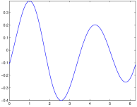
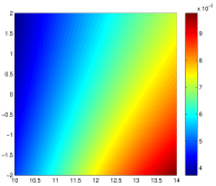
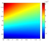
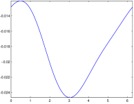
Figure 2: Numerical results in the two-dimensional case. From top left to bottom right: the minimal energy source function $f(\varphi)$, the relative difference between generated and desired fields in the neighborhoods of region $D_{1}$, $D_{2}$, generated field on $\partial D$.

In the three-dimensional case, we observe very similar results. Given an arbitrary point ${\bf x}_{1}=(10,0,0)$ we considered Question  1 with $N=1$, $\delta=1$, $u_{0}=0$, $u_{1}=\frac{1}{|{\bf x}|}$, $D_{1}=B_{2}({\bf x}_{1})$ and $D=B_{15}({\bf 0})$. The accuracy parameter is again $\varepsilon=10^{-3}(\|u_{1}\|_{L^{2}(D_{1})}+\|u_{0}\|_{L^{2}(\partial D)})$. The results are shown in Fig. 3. On the left plot, we show the minimal energy source $h(\theta,\varphi)$ where the unit ball is parameterized using the polar angle $\theta\in[-\pi/2,\pi/2]$ and the azimuth angle $\varphi\in[0,2\pi)$. On the middle plot, we show the difference between the generated field and the desired filed on $\partial B_{2}({\bf x}_{1})$. The right plot shows the difference between the generated field and the desired filed on $\partial B_{15}({\bf 0})$. Due to the limitations of visualization, we are not able to show the difference inside the balls which we observe to be small.

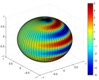
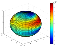
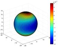
Figure 3: Numerical results in the three-dimensional case. Left: plot of the minimal energy source function $f(\theta,\varphi)$; Middle: plot of the relative difference field on $\partial B_{2}({\bf x}_{1})$; Right: plot of the difference field on $\partial B_{15}({\bf 0})$.

The numerical simulations support our proof that the strategy proposed in this work on generating desired fields in different regions works well. More systematic numerical studies of the problem under various situations, together with a stability analysis will be reported in  [RenOno].

6 Concluding remarks

The idea of manipulating quasistatic fields (or in general acoustic and electromagnetic fields) to generate desired scattering effects has been explored extensively in the engineering community recently due to its practical importance. In this work we present a systematic method to analyze mathematically and numerically the feasibility of the active field manipulation strategy. In the quasistatic regime, we show that one can find source functions that are able to generate desired quasistatic field in multiple regions of interests, to any given accuracy. This enable us to use the active source to create desired illusions or energy focusing without being detected by observations performed outside of the domain of interests. In fact, we show that for any given accuracy, there are infinitely many sources that can achieve the same effects. The source function that has the minimal energy is probably the one that is physically relevant and is weakly stable. Our numerical simulations confirm that the strategy can indeed be realized.

The formulation that we present is independent of the spatial dimension it provides a first step towards the development of field manipulation techniques in more complicated settings, such as in low-to-medium frequency acoustic and TE or TM electromagnetic regimes even though the analysis in those regimes need to be done carefully due to the change of the integral kernels and the presence of resonances. In addition, if the problem is posed in a non-homogeneous medium, with known medium property, the same formulation can be constructed and the same type of minimal energy solution can be obtained through the Euler-Lagrange equation (4.41).

Another essential discussion is about the stability of the solution. As it is well known the problem of inverting a compact operator is highly unstable and that is why we focus on the most physical relevant solution, namely the unique minimum energy solution. By using the generalized discrepancy principle it can be shown that this solution is $L^{2}$ stable with respect to small errors at the antennas or in the measurements of the right hand side data. The $L^{2}$ stability analysis together with the associated numerical discussion for the minimal norm solution will be presented in  [37].

There are many potential applications of the method as we mentioned in the Introduction. Formulation A with $u_{1}=0$ corresponds to the problem of the quasistatic active exterior cloaking as described in [10]. It has been shown in [10, 11](see also [12, 9] for acoustics) that with a few active point sources, one can generate similar effects as what we propose here. This is not surprising because of the non-uniqueness nature of the problem. Indeed, we believe that the cases in [10, 11] are special cases of the current framework, if we are allowed to use continuous functions to approximate the delta function model of point sources. Numerically, this can be done by searching for solutions with minimal $L^{1}$ norm instead of the $L^{2}$ norm (the energy norm). The numerical techniques of $l^{1}$ minimization can then be employed to solve the minimization problem.

Appendix

Lemma 6.1.

Let $0<R_{1}<R_{*}<R_{2}$ be three constants and ${\bf y}_{0}\in{\mathbb{R}}^{d}$ an arbitrary point. Let $f,g\in C(\partial B_{R_{*}}({\bf y}_{0}))$ and define $v_{i}\in C^{2}(B_{R_{*}}({\bf y}_{0}))\cap C^{1}(\overline{B}_{R_{*}}({\bf y}_{0}))$ and $v_{e}\in C^{2}({\mathbb{R}}^{d}\setminus\overline{B}_{R_{*}}({\bf y}_{0}))\cap C^{1}({\mathbb{R}}^{d}\setminus B_{R_{*}}({\bf y}_{0}))$ to be the solutions of the following interior and exterior Dirichlet problems respectively,

$$\left\{\begin{array}[]{ll}\Delta v_{i}=0\mbox{ in }B_{R_{*}}({\bf y}_{0})\vspace{0.15cm}\\ v_{i}=f\mbox{ on }\partial B_{R_{*}}({\bf y}_{0})\vspace{0.15cm}\end{array}\right.$$ (6.44)

nd

$$\left\{\begin{array}[]{lll}\Delta v_{e}=0\mbox{ in }{\mathbb{R}}^{d}\setminus\bar{B}_{R_{*}}({\bf y}_{0})\vspace{0.15cm}\\ v_{e}=g\mbox{ on }\partial B_{R_{*}}({\bf y}_{0})\vspace{0.15cm}\\ v_{e}=\left\{\begin{array}[]{ll}O(1)\mbox{ for }|{\bf x}|\rightarrow\infty,\mbox{ if }d=2\vspace{0.15cm}\\ o(1)\mbox{ for }|{\bf x}|\rightarrow\infty,\mbox{ if }d=3\end{array}\right.\end{array}\right.$$ (6.45)

hen we have,

$$(i)\;\displaystyle\|v_{i}\|_{C(B_{R_{1}}({\bf y}_{0}))}\leq\frac{R_{*}+R_{1}}{|B_{1}|R_{*}(R_{*}-R_{1})^{d-1}}\|f\|_{L^{1}(\partial B_{R_{*}}({\bf y}_{0}))}$$

$$(ii)\;\displaystyle\|v_{e}\|_{C({\mathbb{R}}^{d}\setminus B_{R_{2}}({\bf y}_{0}))}\leq\frac{R_{2}+R_{*}}{|B_{1}|R_{*}(R_{2}-R_{*})^{d-1}}\|g\|_{L^{1}(\partial B_{R_{*}}({\bf y}_{0}))}$$

where $|B_{1}|$ denotes the volume of the unit ball $B_{1}({\bf y}_{0})$.

Proof.

Without loss of generality, we assume that the three balls are centered in the origin, i.e., ${{\bf y}}_{0}={{\bf 0}}$. In this condition, form the Poisson formula we have,

$$v_{i}({\bf x})=\frac{1}{|B_{1}|}\int_{\partial B_{R_{*}}({\bf 0})}f({\bf y})\;\frac{R_{*}^{2}-|{\bf x}|^{2}}{R_{*}|{\bf x}-{\bf y}|^{d}}\;ds_{{\bf y}},\mbox{ for }|{\bf x}|<R_{*}$$ (6.46)

and

$$v_{e}({\bf x})=\frac{1}{|B_{1}|}\int_{\partial B_{R_{*}}({\bf 0})}g({\bf y})\;\frac{|{\bf x}|^{2}-R_{*}^{2}}{R_{*}|{\bf x}-{\bf y}|^{d}}\;ds_{{\bf y}},\mbox{ for }|{\bf x}|>R_{*}$$ (6.47)

where $|B_{1}|$ denotes the volume of the $d$-dimensional unit ball. Recall that the triangle inequality states,

$$|{\bf x}-{\bf y}|\geq||{\bf x}|-|{\bf y}||,\mbox{ for all }{\bf x},{\bf y}\in{\mathbb{R}}^{d}$$ (6.48)

From (6.46) and (6.48) we obtain

$$|v_{i}({\bf x})|\leq\frac{1}{|B_{1}|}\int_{\partial B_{R_{*}}({\bf 0})}|f({\bf y})|\frac{R_{*}+|{\bf x}|}{R_{*}|R_{*}-|{\bf x}||^{d-1}}ds_{{\bf y}},\mbox{ for }|{\bf x}|<R_{*}$$

Thus

$$|v_{i}({\bf x})|\leq\frac{R_{*}+R_{1}}{|B_{1}|R_{*}(R_{*}-R_{1})^{d-1}}\int_{\partial B_{R_{*}}({\bf 0})}|f({\bf y})|ds_{{\bf y}},\mbox{ for }|{\bf x}|\leq R_{1}$$ (6.49)

From (6.47) and (6.48) similarly we obtain

$$|v_{e}({\bf x})|\leq\frac{1}{|B_{1}|}\int_{\partial B_{R_{*}}({\bf 0})}|g({\bf y})|\frac{R_{*}+|{\bf x}|}{R_{*}||{\bf x}|-R_{*}|^{d-1}}ds_{{\bf y}},\mbox{ for }|{\bf x}|>R_{*}$$

and this implies

$$|v_{e}({\bf x})|\leq\frac{R_{*}+|{\bf x}|}{|B_{1}{R_{*}||{\bf x}|-R_{*}|^{d-1}}}\int_{\partial B_{R_{*}}({\bf 0})}|g({\bf y})|ds_{{\bf y}},\mbox{ for }|{\bf x}|>R_{*}.$$

By using simple algebra the last inequality becomes

$$|v_{e}({\bf x})|\leq\frac{1}{|B_{1}|R_{*}}\left(\frac{1}{(|{\bf x}|-R_{*})^{d-2}}+\frac{2R_{*}}{(|{\bf x}|-R_{*})^{d-1}}\right)\int_{\partial B_{R_{*}}({\bf 0})}|g({\bf y})|ds_{{\bf y}},\mbox{ for }|{\bf x}|>R_{*}.$$

and, similarly as for (6.49) this implies

$$|v_{e}({\bf x})|\leq\frac{1}{|B_{1}|R_{*}}\left(\frac{1}{(R_{2}-R_{*})^{d-2}}+\frac{2R_{*}}{(R_{2}-R_{*})^{d-1}}\right)\int_{\partial B_{R_{*}}({\bf 0})}|g({\bf y})|ds_{{\bf y}},\mbox{ for }|{\bf x}|\geq R_{2}.$$ (6.50)

The statement of the Lemma is implied by (6.49), and (6.50). ∎

The next result is classical but for the self contained character of the paper we choose to include it here.

Lemma 6.2.

The operator $K$ defined in (3.8) is a compact linear operator from $L^{2}(\partial B_{\delta}({\bf 0}))$ to $\Xi$.

Proof.

Let $\{u_{n}\}$ be a bounded sequence in $L^{2}(\partial B_{\delta}({\bf 0}))$, i.e.,

$$\|u_{n}\|_{L^{2}(\partial B_{\delta}({\bf 0}))}\leq C$$ (6.51)

with $C$ independent of $n$. Then there exists $u\in L^{2}(\partial B_{\delta}({\bf 0}))$ such that, up to a subsequence still indexed by $n$, we have

$$u_{n}\rightharpoonup u,\mbox{ weekly in }L^{2}(\partial B_{\delta}({\bf 0}))$$ (6.52)

Moreover, (6.51) and (6.52) imply,

$$\|u\|_{L^{2}(\partial B_{\delta}({\bf 0}))}\leq C$$ (6.53)

From the continuity of the kernels of $K_{1}$ and $K_{2}$ defined at (3.9) and by using (6.52) we obtain,

$$K_{1}u_{n}({\bf x}) \rightarrow K_{1}u({\bf x}),\mbox{ for all }{\bf x}\in\partial B_{a^{\prime}}({\bf x}_{0})$$

$$K_{2}u_{n}({\bf z}) \rightarrow K_{2}u({\bf z}),\mbox{ for all }{\bf z}\in\partial B_{R^{\prime}}({\bf 0})$$ (6.54)

Next observe that

$$\frac{\partial\Phi({\bf x},{\bf y})}{\partial\mbox{\boldmath${\nu}$}_{{\bf y}}}=\frac{1}{|B_{1}|}\frac{({\bf x}-{\bf y})\cdot{\bf y}}{\delta|{\bf x}-{\bf y}|^{d}},\mbox{ for }{\bf y}\in\partial B_{\delta}({\bf 0})\mbox{ and for any }{\bf x}\neq{\bf y}$$ (6.55)

where again $|B_{1}|$ is the volume of the $d$-dimensional unit ball and we used here that $\displaystyle\mbox{\boldmath${\nu}$}_{{\bf y}}=\frac{{\bf y}}{|{\bf y}|}$ on $\partial B_{\delta}({\bf 0})$. From (6.51), (6.52), (6.53) and (6.55) we have

$$|K_{1}(u_{n}-u)({\bf x})| = \left|\displaystyle\int_{\partial B_{\delta}({\bf 0})}(u_{n}-u)({\bf y})\frac{\partial\Phi({\bf x},{\bf y})}{\partial\mbox{\boldmath${\nu}$}_{{\bf y}}}ds_{{\bf y}}\right|$$ (6.56)

$$\leq \|u_{n}-u\|_{L^{2}(\partial B_{\delta}({\bf 0}))}\left\|\frac{\partial\Phi({\bf x},{\bf y})}{\partial\mbox{\boldmath${\nu}$}_{{\bf y}}}\right\|_{L^{2}(\partial B_{\delta}({\bf 0}))}$$

$$\leq \displaystyle C\left(\frac{1}{|{\bf x}_{0}|-a^{\prime}-\delta}\right)^{d-1}\;\;\;\;\mbox{ for }{\bf x}\in\partial B_{a^{\prime}}({\bf x}_{0})$$

where we used that

$$\mbox{dist}(\partial B_{a^{\prime}}({\bf x}_{0}),\partial B_{\delta}({\bf 0}))=|{\bf x}_{0}|-a^{\prime}-\delta>0$$

with $|{\bf x}_{0}|-a^{\prime}-\delta>0$ following from (2.4).

Similarly as for (6.56), from (6.51), (6.52) (6.55) we obtain,

$$|K_{2}(u_{n}-u)({\bf x})| = \left|\displaystyle\int_{\partial B_{\delta}({\bf 0})}(u_{n}-u)({\bf y})\frac{\partial\Phi({\bf z},{\bf y})}{\partial\mbox{\boldmath${\nu}$}_{{\bf y}}}ds_{{\bf y}}\right|$$ (6.57)

$$\leq \|u_{n}-u\|_{L^{2}(\partial B_{\delta}({\bf 0}))}\left\|\frac{\partial\Phi({\bf z},{\bf y})}{\partial\mbox{\boldmath${\nu}$}_{{\bf y}}}\right\|_{L^{2}(\partial B_{\delta}({\bf 0}))}$$

$$\leq \displaystyle C\frac{1}{(R^{\prime}-\delta)}\;\;\;\;\mbox{ for }{\bf z}\in\partial B_{R^{\prime}}({\bf 0})$$

where we used that

$$\mbox{dist}(\partial B_{R^{\prime}}({\bf 0}),\partial B_{\delta}({\bf 0}))=R^{\prime}-\delta>0$$

From (6.54), (6.56) and (6.57) and the Lebesgue dominated convergence theorem, we obtain

$$K_{1}u_{n}\rightarrow K_{1}u \mbox{ strongly in }L^{2}(\partial B_{a^{\prime}}({\bf x}_{0}))$$

$$K_{2}u_{n}\rightarrow K_{2}u \mbox{ strongly in }L^{2}(\partial B_{R^{\prime}}({\bf 0}))$$ (6.58)

Then from the definition of the operator $K$ and from (6.58) we conclude that

$$Ku_{n}\rightarrow Ku\mbox{ strongly in }\Xi$$

and this implies the statement of the lemma. ∎

References

• [1] A. Alu and N. Engheta, Plasmonic and metamaterial cloaking: physical mechanism and potentials, J. Opt. A: Pure Appl. Opt, 10, (2008).
• [2] H. Brezis, Analyse functionnelle. Theorie et applications, Dunod, Paris, France, 2nd ed., (1999).
• [3] H. Chen and C. Chan, Acoustic cloaking and transformation acoustics, J. Phys. D: Appl. Phys., 43, (2010).
• [4] H. Chen, C. T. Chan, and P. Sheng, Transformation optics and metamaterials, Nature Materials, 9, pp. 387–396, (2010).
• [5] D. Colton and R. Kress, Inverse Acoustic and Electromagnetic Scattering Theory, Springer-Verlag, New York, (1998).
• [6] S. A. Cummer, B.-I. Popa, D. Schurig, D. R. Smith, J. Pendry, M. Rahm, and A. Starr, Scattering theory derivation of a 3d acoustic cloaking shell, Phys. Rev. Lett., 100, (2008).
• [7] A. Greenleaf, Y. Kurylev, M. Lassas, and G. Uhlmann, Invisibility and inverse problems, Bull. Amer. Math. Soc., 46, pp. 55–97, (2009).
• [8] A. Greenleaf, M. Lassas, and G. Uhlmann, Anisotropic conductivities that cannot be detected by eit, Physiol. Meas., 24, pp. 413–419, (2003).
• [9] F.  Guevara Vasquez, G. W. Milton, D. Onofrei, P. Seppecher, Transformation elastodynamics and active exterior acoustic cloaking, Acoustic metamaterials: Negative refraction, imaging, lensing and cloaking, arXiv:1105.1221, (2011).
• [10] F. Guevara Vasquez, G. W. Milton, and D. Onofrei, Active exterior cloaking, Phys. Rev. Lett., 103, (2009).
• [11]  , Broadband exterior cloaking, Optics Express, 17, pp. 14800–14805, (2009).
• [12]  , Exterior cloaking with active sources in two dimensional acoustics, accepted Wave Motion, arXiv:1009.2038, (2011).
• [13] A. Kirsch, An Introduction to the Mathematical Theory of Inverse Problems, Springer-Verlag, New York, (1996).
• [14] R. Kohn, D. Onofrei, M. Vogelius, and M. Weinstein, Cloaking via change of variables for the helmholtz equation at fixed frequency, Comm. Pure. Appl. Math., 63, pp. 973–1016, (2000).
• [15] R. Kress, Linear Integral Equations, Applied Mathematical Sciences, Springer-Verlag, New York, 2nd ed., (1999).
• [16] Y. Lai, H. Chen, Z.-Q. Zhang, and C. T. Chan, Complementary media invisibility cloak that cloaks objects at a distance outside the cloaking shell, Phys. Rev. Lett., 102, (2009).
• [17] U. Leonhardt, Notes on conformal invisibility devices, New J. Phys., 8, p. 118, (2006).
• [18]  , Optical conformal mapping, Science, 312, pp. 1777–1780, (2006).
• [19] D. A. B. Miller, On perfect cloaking, Opt. Express, 14, pp. 12457–12466, (2006).
• [20] G. W. Milton and N.-A. P. Nicorovici, On the cloaking effects associated with anomalous localized resonance, Proc. R. Soc. Lon. Ser. A. Math. Phys. Sci., 462, pp. 3027–3059, (2006).
• [21] G. W. Milton, N.-A. P. Nicorovici, R. C. McPhedran, K. Cherednichenko, and Z. Jacob, Solutions in folded geometries, and associated cloaking due to anomalous resonance, New J. Phys., 10, (2008).
• [22] N.-A. P. Nicorovici, G. Milton, R. C. McPhedran, and L. C. Botten, Quasistatic cloaking of two-dimensional polarizable discrete systems by anomalous resonance, Opt. Express, 15, pp. 6314–6323, (2007).
• [23] J. B. Pendry, D. Schurig, and D. R. Smith, Controlling electromagnetic fields, Science, 312, pp. 1780–1782, (2006).
• [24] I. I. Smolyaninov, V. N. Smolyaninova, A. V. Kildishev, and V. M. Shalaev, Anisotropic metamaterials emulated by tapered waveguides: Application to optical cloaking, Phys. Rev. Lett., 103, (2009).
• [25] Hoai-Minh Nguyen, Approximate cloaking for the Helmholtz equation via transformation optics and consequences for perfect cloaking, to appear in Comm. Pure Appl. Math , Comm. Pure. Appl. Math., Volume 65, Issue 2, pages 155–186, (2012).
• [26] H. Y. Liu, Virtual reshaping and invisibility in obstacle scattering, Inverse Problems, 25, 045006, (2009).
• [27] Hongyu Liu, Hongpeng Sun, Enhanced Near-cloak by FSH Lining, online at arXiv:1110.0752, (2011).
• [28] Hongyu Liu, Ting Zhou, On Approximate Electromagnetic Cloaking by Transformation Media , SIAM J. Appl. Math., 71, pp. 218–241, (2011).
• [29] L. S. Dolin, On a possibility of comparing three-dimensional electromagnetic systems with inhomogeneous filling, Izv. Vyssh. Uchebn. Zaved. Radiofiz. 4, 964, (1961).
• [30] E. J. Post, Formal structure of electromagnetics, North-Holland (1962).
• [31] M. Lax and D. F. Nelson, “Maxwell equations in material form,” Phys. Rev. B 13, 1777, (1976).
• [32] H. Ammari, Hyeonbae Kang, Hyundae Lee, Mikyoung Lim,Enhancement of near-cloaking. Part II: the Helmholtz equation, To appear in Communications in Mathematical Physics, (2012).
• [33] H. Ammari, J. Garnier, V. Jugnon, H. Kang, H. Lee, and M. Lim, Enhancement of near-cloaking. Part III: numerical simulations, statistical stability, and related questions. To appear in Contemporary Mathematics (2012).
• [34] H. Ammari, H. Kang, H. Lee, and M. Lim, Enhancement of near-cloaking using generalized polarization tensors vanishing structures. Part I: The conductivity problem. to appear in Communications in Mathematical Physics (2012).
• [35] J. Valentine, Z. Shuang, T. Zentgraf, Z. Xiang Development of Bulk Optical Negative Index Fishnet Metamaterials: Achieving a Low-Loss and Broadband Response Through Coupling, Proceedings of the IEEE, Vol. 99, Iss. 10 pp. 1682 - 1690, (2011).
• [36] Allan Greenleaf, Yaroslav Kurylev, Matti Lassas, Gunther Uhlmann, Schrodinger’s Hat: Electromagnetic, acoustic and quantum amplifiers via transformation optics, online at arxiv.org: arXiv:1107.4685v1, 2011.
• [37] D. Onofrei, On the stability of the active field manipulation design, in preparation, (2012).
• [38] N. Peake, D.G. Crighton, Active control of sound, Annu. Rev. Fluid Mech., vol.32, 137-164, (2000).
• [39] S.J. Elliot, P.A. Nelson, The active control of sound, Electronics and Comm. Engineering Journal, August, (1990).
• [40] J. Loncaric, V.S. Ryaben’kii, S.V. Tsynkov, Active shielding and control of environmental noise, technical report, NASA/CR-2000-209862, ICASE Report No. 2000-9, (2000).
• [41] J. Loncaric, S.V. Tsynkov, Quadratic optimization in the problems of active control of sound, Appl. NUm. Math., vol. 52, 381-400, 2005.
• [42] A.W. Peterson, S.V. Tsynkov, Active control of sound for composite regions, SIAM J. Appl. Math, vol. 67, Iss. 6, pp 1582-1609, (2007).
• [43] C.R. Fuller, A.H. von Flotow, Active control of sound and vibration, IEEE, (1995).
• [44] P. Leug, Process of silencing sound oscillations, U.S. patent no. 2043416, (1936).
• [45] H.F. Olson, E.G. May, Electronic sound absorber, J. Acad. Soc. America, vol. 25, pp. 1130-1136, (1953).
• [46] A. Greenleaf, Y. Kurylev, M. Lassas, G. Uhlmann, Cloaking a Sensor via Transformation Optics, Physical Review E 83, 016603 (2011).
• [47] Giuseppe Castaldi, Ilaria Gallina, Vincenzo Galdi, Andrea Alu, Nader Engheta, Power scattering and absorption mediated by cloak/anti-cloak interactions: A transformation-optics route towards invisible sensors, JOSA B, Vol. 27, Iss. 10, pp. 2132-2140, (2010).
• [48] H. H. Zheng, J. J. Xiao, Y. Lai, C. T. Chan Exterior optical cloaking and illusions by using active sources: A boundary element perspective, Phys. Rev. B, Vol. 81, Issue 19, 2010.