Error Analysis regarding the calculation of Nonlinear Force-free Field

Abstract

Magnetic Field extrapolation is an alternative method to study chromospheric and coronal magnetic fields. In this paper, two semi-analytical solutions of force-free fields (Low and Lou, 1990) have been used to study the errors of nonlinear force-free (NLFF) fields based on force-free factor $\alpha$. Three NLFF fields are extrapolated by approximate vertical integration (AVI) Song et al. (2006), boundary integral equation (BIE) Yan and Sakurai (2000) and optimization (Opt.) Wiegelmann (2004) methods. Compared with the first semi-analytical field, it is found that the mean values of absolute relative standard deviations (RSD) of $\alpha$ along field lines are about 0.96-1.19, 0.63-1.07 and 0.43-0.72 for AVI, BIE and Opt. fields, respectively. While for the second semi-analytical field, they are about 0.80-1.02, 0.67-1.34 and 0.33-0.55 for AVI, BIE and Opt. fields, respectively. As for the analytical field, the calculation error of $\langle|RSD|\rangle$ is about 0.1 $\sim$ 0.2. It is also found that RSD does not apparently depend on the length of field line. These provide the basic estimation on the deviation of extrapolated field obtained by proposed methods from the real force-free field.

Keywords Magnetic Fields, Photosphere, Corona

1 Introduction

The magnetic field plays key roles in a variety of dynamical processes, particularly in eruptive phenomena such as filament eruptions, flares and coronal mass ejections. The topological structure is an important properties of spatial magnetic field. Therefore it is important to understand three-dimensional properties of magnetic field in order to elaborate efficient theoretical models, which will contribute to understand solar activity. At present, due to the restrictions of observational technique, we can not get the accurate information on magnetic field in the hot and tenuous corona. This can only be done at the level of the cooler and denser photosphere. In spite of that, the extrapolation of magnetograms, measured maps of the photospheric or low chromospheric field, into the corona is the most important technique to supply the missing information about the spatial magnetic field. The field extrapolation is based on force-free assumption (Aly, 1989), which assumes that the corona is free of Lorentz forces. For the low-$\beta$ corona where the plasma is tenuous, the force-free assumption is appropriate. The force-free field obeys the following equations:

$$\nabla\times\textbf{B}=\alpha(\textbf{r})\textbf{B},$$ (1)

$$\nabla\cdot\textbf{B}=0,$$ (2)

where $\alpha$ is called force-free factor. If $\alpha$ = 0, the equations represent a potential field (a current-free field). If $\alpha$ = constant, they describe a current-carrying linear force-free (LFF) field, and if $\alpha$ = $f(\textbf{r})$ it is a general NLFF field. This two equations also imply that:

$$\textbf{B}\cdot\nabla\alpha=0.$$ (3)

Equation (3) demonstrates that $\alpha$ is invariant along field lines of B. The scalar $\alpha$ is in general a function of space and identifies how much current flows along each field line. Thus, the deviations of $\alpha$ along one field line at some extent can demonstrate performance of field extrapolation.

At present, the potential ($\alpha$ = 0) and linear force-free ($\alpha$ = constant) field extrapolations reached a mature development, but they describe the magnetic field above the photosphere in a very restricted manner. According to the practice conditions of solar magnetic field, it is not a current-free field and NLFF should be more reasonable. Recently, several NLFF field extrapolation methods have been proposed ($e.g.$, Wu et al., 1990; Cuperman et al., 1990; Démoulin et al., 1992; Mikic and McClymont, 1994; Roumeliotis, 1996; Amari et al., 1997; Sakurai, 1981; Chodura and Schlueter, 1981; Yan and Sakurai, 2000; Wheatland et al., 2000; Wiegelmann, 2004; Song et al., 2006; He and Wang, 2008). The performance of above extrapolation methods have been studied in several papers ($e.g.,$ Schrijver et al., 2006; Amari et al., 2006; Régnier et al., 2004; Yan and Li, 2006; Wiegelmann et al., 2006 Valori et al., 2007; Régnier et al., 2007; DeRosa et al., 2009; He et al., 2011 and Liu et al. 2011 ), comparing to models or observations ($e.g.$, the appearance of extreme ultraviolet (EUV) and X-ray or loops) those methods above mentioned can give reasonable results at the level of macroscopic structure.

Since the field extrapolation is an important technique to study the coronal magnetic field, the performance of field extrapolation become special importance. From Equation (3), it can been seen that though $\alpha$ may change from one field line to another, it must be a constant along one field line. Knowing $\alpha$ is an important parameter worthy to be researched, in this paper the distributions of $\alpha$ between extrapolated field and semi-analytical field are compared; the calculation error of $\alpha$ is discussed; the performance of $\alpha$ along field line are studied specially.

The paper is organized as follows: firstly, the description of extrapolation methods and semi-analytical field will be introduced in Section 2; secondly, the results of distribution comparison and calculation error of force-free factor $\alpha$ are shown in Section 3; at last, the short discussions and conclusions will be given in section 4.

2 Extrapolation methods and Semi-analytical field

2.1 Approximate vertical integration method

The approximate vertical integration (AVI) method (Song et al., 2006) was improved from the vertical integration proposed by Wu et al. (1990). In this method, it is assumed that the magnetic field components is given by the following formula,

$$\textbf{B}_{x}=\xi_{1}(x,y,z)F_{1}(x,y,z),$$ (4)

$$\textbf{B}_{y}=\xi_{2}(x,y,z)F_{2}(x,y,z),$$ (5)

$$\textbf{B}_{z}=\xi_{3}(x,y,z)F_{3}(x,y,z),$$ (6)

assuming the second-order continuous partial derivatives in a certain height range, 0$<z<$H (H is the calculated height from the photospheric surface). In Equations (4)-(6), $\xi_{1},\xi_{2}$ and $\xi_{3}$ mainly depend on $z$ and slowly vary with $x$ and $y$, while $F_{1},F_{2}$ and $F_{3}$ mainly depend on $x$ and $y$ and weakly vary with $z$. After constructing the magnetic field, the following integration equations,

$$\dfrac{\partial B_{x}}{\partial z}=\dfrac{\partial B_{z}}{\partial x}+\alpha B_{y},$$ (7)

$$\dfrac{\partial B_{y}}{\partial z}=\dfrac{\partial B_{z}}{\partial y}-\alpha B_{x},$$ (8)

$$\dfrac{\partial B_{z}}{\partial z}=-\dfrac{\partial B_{x}}{\partial x}-\dfrac{\partial B_{y}}{\partial y},$$ (9)

$$\alpha B_{z}=\dfrac{\partial B_{y}}{\partial x}-\dfrac{\partial B_{x}}{\partial y},$$ (10)

can be used to calculate extrapolated field. There exists singularity problem due to differential operation for AVI method, hence we smooth data locally where exists singularity (cf. Liu et al., 2011).

2.2 Boundary integral equation method

The boundary integral equation (BIE) method proposed by Yan and Sakurai (2000), which uses the integration function to extrapolate the magnetic field. In this method, an optimized parameter $\lambda$, which is the function of spatial position x, must be found through iteration. The integral

$$\textbf{B}(x_{i},y_{i},z_{i})=\int_{\Gamma}\dfrac{z_{i}[\lambda r\sin(\lambda r)+\cos(\lambda r)]\textbf{B}_{0}(x,y,0)}{2\pi[(x-x_{i})^{2}+(y-y_{i})^{2}+z_{i}^{2}]^{3/2}},$$ (11)

is used to calculate the magnetic field, where $r$ = $[(x-x_{i})^{2}+(y-y_{i})^{2}+z_{i}^{2}]^{1/2}$ and $\textbf{B}_{0}$ is the magnetic field of photospheric surface. This method is to find suitable values of $\lambda$ through iteration and try to make sure that the extrapolated field is force-free and divergence-free (cf. He and Wang, 2008 and Li, Yan, and Song, 2004).

2.3 Optimization method

The optimization (Opt.) method proposed by Wheatland et al. (2000) and developed by Wiegelmann (2004) consists in minimizing a joint measure for the normalized Lorentz force and the divergence of the field, given by the function,

$$L=\int_{V}\omega(x,y,z)[B^{-2}|(\nabla\times\textbf{B}\times\textbf{B})|^{2}+|\nabla\cdot\textbf{B}|^{2}]d^{3}x,$$ (12)

where $\omega(x,y,z)$ is a weighting function related position. It is clear that (for $w>0$) the force-free equations are fulfilled when $L$ is equal to zero. This method involves minimizing $L$ by optimizing the solution function $\textbf{B}(x,t)$ through states that are increasingly force- and divergence-free, where $t$ is an artificial time-like parameter introduced.

2.4 Semi-analytical NLFF Field

Low and Lou (1990) have presented a class of axis-symmetric NLFF fields in the spherical coordinate system. These NLFF field can be used to test the performance of field extrapolation by shifted under two steps of Cartesian coordinate system transformation, rotating by an angle $\phi$ around the y-axis and moving the origin to a distance $l$ along the z-axis. A special class of NLFF fields denoted B($n$, $m$) can be obtained in the spherical coordinate system. For different $n$ and $m$, it can give different distributions of magnetic field, which meet the requirements of divergence-free and force-free equations. Then we should specify two parameters $l$ and $\phi$ for coordinate transformation. In this paper we choose such two classic NLFF fields as semi-analytical fields:

SAF1: the semi-analytical field with $n=1,m=1$, $l=0.3$, and $\phi=\dfrac{\pi}{4}$, set $x\in[-0.5,0.5]$, $y\in[-0.5,0.5]$ and $z\in[0,1]$ in the Cartesian coordinate system.

SAF2: the semi-analytical field with $n=3,m=1$, $l=0.3$, and $\phi=\dfrac{4\pi}{5}$, set $x\in[-0.5,0.5]$, $y\in[-0.5,0.5]$ and $z\in[0,1]$ in the Cartesian coordinate system.

The mesh is 64 $\times$ 64 $\times$ 64 for those two fields. Because $\alpha$ will be studied mainly, the values of analytical $\alpha$ ($\alpha_{Ana.}$) of SAF1 and SAF2 are calculated (cf. Low and Lou, 1990) and saved in 3D position.

3 Results

3.1 SAF1

Figure 1 shows the field lines of SAF1, AVI ,BIE and Opt. fields. It can be found that the distributions of field lines of extrapolated fields (AVI, BIE or Opt. field) are basically consistent with that of SAF1, and the field lines of AVI and BIE fields are very similar. Hence the structure of spatial field obtained from field extrapolation can present for that of semi-analytical field at some extent. In order to evaluate the performance of extrapolated field, we calculate the average ($\langle|F|\rangle$) and maximum ($F_{max}$) Lorentz-force (J $\times$ $\textbf{B}/\mu_{0}$, $\mu_{0}$ is permeability) and $\sigma_{j}$, defined by equation (13) same as Schrijver et al. (2006), to test the extent of force-free for each extrapolated field. The results of these physical quantity are given in table 1 for SAF1 and the corresponding extrapolated fields, here the pixel size is assumed 1 arcsec. It can be found that angles between J and B of Opt. field (comparable to SAF1 at some extent) are smaller than those of AVI and BIE fields.

$$\sigma_{J}=\left(\sum_{i}\dfrac{|\textbf{J}_{i}\times\textbf{B}_{i}|}{B_{i}}\right)/\sum_{i}J_{i},$$ (13)

Table 1 : The results of the average ($\langle|F|\rangle$) and maximum ($F_{max}$) Lorentz-force and $\sigma_{j}$ for SAF1 and the corresponding extrapolated fields.

	$\langle|F|\rangle$	$F_{max}$	$\sigma_{J}$
	($G^{2}/M$)$\times$ $10^{-14}$	($G^{2}/M$)$\times$ $10^{-12}$
SAF1	2.2	0.8	0.14
AVI	5.6	9.6	0.72
BIE	3.7	5.4	0.45
Opt.	2.3	2.4	0.21

Because a 3D field is available, force-free factor $\alpha$ can be calculated individually from the formulas (14)-(16), which are obtained by expanding Equation (1). Because $\alpha$ is the scalar depended on spatial position, $\alpha_{1}$, $\alpha_{2}$ and $\alpha_{3}$ should be the same for a given position. Figure 2 shows the images of $\alpha_{1}$, $\alpha_{2}$ and $\alpha_{3}$, magnetic field components and current components ($J_{x}$, $J_{y}$, $J_{z}$) labeled for SAF1 at $z=0$, where the red lines on each grey-scale map of magnetic field component are the neutral line of each component labeled. Because $\alpha$ is calculated from the semi-analytical field, this figure demonstrates that there will be unavoidable calculation errors when $\alpha$ is calculated from magnetic field. The evident calculation errors are most likely located near where the magnetic field components reversed, which are consistent among $\alpha_{1}$, $\alpha_{2}$ and $\alpha_{3}$. From the formulas (14)-(16), it can be seen that there are singularity problem when magnetic field component approaches to zero, hence the evident calculation errors correspond to the neutral line of magnetic field components (red lines labeled). Since $\alpha$ is a scalar and the function of spatial position, it is reasonable to combine $\alpha_{1}$, $\alpha_{2}$ and $\alpha_{3}$ to minimize the calculation errors.

$$\alpha_{1}=J_{x}/B_{x},\hskip 21.52771ptJ_{x}=\left(\dfrac{\partial B_{z}}{\partial y}-\dfrac{\partial B_{y}}{\partial z}\right)\bigg{/}B_{x},$$ (14)

$$\alpha_{2}=J_{y}/B_{y},\hskip 21.52771ptJ_{y}=\left(\dfrac{\partial B_{x}}{\partial z}-\dfrac{\partial B_{z}}{\partial x}\right)\bigg{/}B_{y},$$ (15)

$$\alpha_{3}=J_{z}/B_{z},\hskip 21.52771ptJ_{z}=\bigg{(}\dfrac{\partial B_{y}}{\partial x}-\dfrac{\partial B_{x}}{\partial y}\bigg{)}\bigg{/}B_{z}.$$ (16)

In order to compare $\alpha$, the combined value from $\alpha_{1}$, $\alpha_{2}$ and $\alpha_{3}$ is also studied in this work. The method to realize this is that: to get the average of two values of $\alpha$ ($\alpha_{1}$, $\alpha_{2}$ or $\alpha_{3}$) whose values are closed, which means that for a given position $\alpha$ deduced from one formula (14, 15 or 16) is give up forcibly. Figure 3 shows the process to combine $\alpha$ reasonably. It shows $\alpha_{1}$, $\alpha_{2}$ and $\alpha_{3}$, the combined $\alpha$ ($\alpha_{Com.}$) and analytical $\alpha$ ($\alpha_{Ana.}$) of SAF1 at $z=0$, $z=1$ and $z=2$. It is found that there are evident calculation errors for $\alpha_{1}$, $\alpha_{2}$ and $\alpha_{3}$. The correlation coefficients between $\alpha_{1,2,3,Com.}$ and $\alpha_{Ana.}$ are given in table 2. However $\alpha_{Com.}$ is improved evidently, $\alpha_{Com.}$ match very well with $\alpha_{Ana.}$, the correlation coefficients between $\alpha_{Com.}$and $\alpha_{Ana.}$ are 0.99. Therefore the process to combine $\alpha$ is valid for SAF1 (note this validation is not suitable for all cases of extrapolated field, but it can be valid on the whole, which will present next section).

Table 2 : The correlation coefficients between $\alpha_{1,2,3,Com.}$ and $\alpha_{Ana.}$ for SAF1.

	$\alpha_{Com.}$	$\alpha_{1}$	$\alpha_{2}$	$\alpha_{3}$
z=0	0.99	0.97	0.93	0.90
z=1	0.99	0.92	0.89	0.91
z=2	0.99	0.97	0.90	0.93

Figure 4 shows the images of $\alpha_{1,2,3,Com.}$ deduced from SAF1, AVI, BIE and Opt. fields at $z=1$ and $z=2$. There are evident deviations of $\alpha$ between extrapolated field and semi-analytical field. The correlation coefficients of $\alpha_{1,2,3,Com.}$ between SAF1 and each extrapolated fields are given in table 3. This low relation of $\alpha$s between extrapolated field and SAF1 is caused mainly by the deviations between extrapolated field and SAF1, since from the above analysis it is found that the correlation coefficients between $\alpha_{Com.}$ and $\alpha_{Ana.}$ are already greater than 99% for SAF1.

Table 3 : The correlation coefficients of $\alpha_{1,2,3,Com.}$ between SAF1 and the corresponding extrapolated fields.

	AVI	BIE	Opt.
$\alpha_{Com.}(z=1)$	0.36	0.49	0.67
$\alpha_{Com.}(z=2)$	0.42	0.41	0.59
$\alpha_{2}(z=1)$	0.43	0.59	0.62
$\alpha_{2}(z=2)$	0.46	0.46	0.54
$\alpha_{1}(z=1)$	0.33	0.39	0.55
$\alpha_{1}(z=2)$	0.38	0.41	0.56
$\alpha_{3}(z=1)$	0.65	0.45	0.53
$\alpha_{3}(z=2)$	0.58	0.52	0.63

$$RSD=\dfrac{1}{\langle\alpha\rangle}\sqrt{\dfrac{1}{N-1}\sum_{i=0}^{N-1}(\alpha_{i}-\langle\alpha\rangle)^{2}}.$$ (17)

As for the NLFF field, force-free factor $\alpha$ should be a constant along one special field line. Hence a physical quantity: relative standard deviation (RSD), which can estimate the deviation of $\alpha$ along field lines is studied. RSD is defined by formula (17), where N is the number of points calculated along field line. Figure 5(A) shows RSD of $\alpha_{Ana.}$ along each field lines for SAF1. Because the values of RSD approach zero ($\langle|RSD|\rangle$ is only 0.0056 and the points is very concentrated, which can give the conclusion that the field lines can be traced and the deviation of $\alpha_{Ana.}$ of SAF1 is negligible. It means that SAF1 satisfies the force-free equations very well.

In Figure 6, the possibility function (PDF) of RSD of $\alpha_{1,2,3,Com.}$ along some selected field lines are plotted for SAF1, AVI, BIE and Opt. fields. The reason for RSD of SAF1 are plotted is that they can give an estimation on calculation errors. It can be found that PDF of RSD of $\alpha$ is very narrow and $\langle|RSD|\rangle$ is 0.09-0.16 for SAF1, this value can be taken as the calculation error of $\langle|RSD|\rangle$. For extrapolated NLFF fields, there are evident deviations of $\alpha$ along field lines since PDF of RSD of $\alpha$ is not concentrated and $\langle|RSD|\rangle$ of $\alpha$ along some selected field lines is 0.96-1.19, 0.63-1.07 and 0.43-0.72 for AVI, BIE and Opt. field, respectively. Additionally, the validation of combined is not evident for some cases,for example BIE extrapolated field (its RSD of $\alpha_{Com.}$ is not the smallest one). In Figure 7, RSD vs field line length are plotted for SAF1, AVI, BIE and Opt. fields in order to find whether or not RSD are depend on field line length, where field line length was indicated by the number of points calculated along each field line. It can be found that RSD dose basically not depend on field line length.

3.2 SAF2

Figure 8 shows the field lines of SAF2, AVI, BIE and Opt. fields. Same as Figure 1 it can be found that although there are some fine differences of field lines among these fields, the distributions of field lines of extrapolated fields basically match that of SAF2 at large scale. Like SAF1, we also calculate $\langle F\rangle$,  $F_{max}$ and $\sigma_{j}$ for each extrapolated field corresponding to SAF2. The results are given in table 4, here the pixel size is also assumed 1 arcsec. It can be found that for SAF2 angles between J and B are large than those for SAF1, even for semi-analytical field. The $\langle F\rangle$ and $F_{max}$ differences among extrapolated fields are negligible, however the $\sigma_{j}$ of Opt. field is better than those of AVI and BIE fields.

Table 4 : The results of the average ($\langle F\rangle$) and maximum ($F_{max}$) Lorentz-force and $\sigma_{j}$ for SAF2 and the corresponding extrapolated fields.

	$\langle F\rangle$	$F_{max}$	$\sigma_{J}$
	($G^{2}/M$)$\times$ $10^{-12}$	($G^{2}/M$)$\times$ $10^{-11}$
SAF2	1.4	13.6	0.30
AVI	9.3	25.7	0.69
BIE	7.7	32.4	0.71
Opt.	1.8	2.6	0.31

Same as Figure 2 for SAF1, Figure 9 shows the images of $\alpha_{1}$, $\alpha_{2}$ and $\alpha_{3}$, components of magnetic field and current for SAF2 at $z=0$. This also demonstrates that calculation errors are mainly located near where the magnetic field components reversed. Like Figure 3 for SAF1, Figure 10 shows $\alpha_{1}$, $\alpha_{2}$, $\alpha_{3}$, $\alpha_{Com.}$ and $\alpha_{Ana.}$ of SAF2 at $z=0$, $z=1$ and $z=2$. Through calculation we get the correlation coefficients between $\alpha_{1,2,3,Com.}$ and $\alpha_{Ana.}$, which are shown in table 5. It shows that $\alpha_{Com.}$ evidently improve the computational precision of $\alpha$ for SAF2.

Table 5 : he correlation coefficients between $\alpha_{1,2,3,Com.}$ and $\alpha_{Ana.}$ for SAF2.

	$\alpha_{Com.}$	$\alpha_{1}$	$\alpha_{2}$	$\alpha_{3}$
z=0	0.96	0.96	0.92	0.92
z=1	0.99	0.94	0.94	0.94
z=2	0.99	0.93	0.97	0.97

Figure 11 shows the images of $\alpha_{1,2,3,Com.}$ deduced from SAF2, BIE, AVI and Opt. fields at $z=1$ and $z=2$. Comparing the results of SAF1, the consistency between $\alpha$s of extrapolated field and SAF2 is improved at some extent. The correlation coefficients of $\alpha_{1,2,3,Com.}$ between SAF1 and the corresponding extrapolated fields are given in table 6. This relative low relation of $\alpha$s between extrapolated field and SAF2 is also caused by the deviations extrapolated field and semi-analytical field.

Table 6 : The correlation coefficients of $\alpha_{1,2,3,Com.}$ between SAF1 and the corresponding extrapolated fields.

	AVI	BIE	Opt.
$\alpha_{Com.}(z=1)$	0.54	0.77	0.72
$\alpha_{Com.}(z=2)$	0.59	0.73	0.68
$\alpha_{2}(z=1)$	0.48	0.71	0.67
$\alpha_{2}(z=2)$	0.54	0.64	0.54
$\alpha_{1}(z=1)$	0.56	0.65	0.71
$\alpha_{1}(z=2)$	0.51	0.63	0.66
$\alpha_{3}(z=1)$	0.65	0.58	0.68
$\alpha_{3}(z=2)$	0.58	0.55	0.65

Figure 5(B) shows RSD of $\alpha_{Ana.}$ for SAF2, where $\langle|RSD|\rangle$ is 0.0023 and the points is also very concentrated, which also indicate that deviation of $\alpha_{Ana.}$ of SAF2 is negligible. It means that SAF2 also satisfies force-free equations very well.

Same as Figure 6, PDF of RSD of $\alpha$ along some selected field lines are plotted in Figure 12 for SAF2, BIE, AVI and Opt. fields. From this figure, it can be found that calculation errors denoted by RSD, that deduced from SAF2, is smaller than those of SAF1. $\langle|RSD|\rangle$ is 0.13-0.11, 0.80-1.02, 0.67-1.34 and 0.33-0.55 for SAF2, AVI, BIE and Opt. fields, respectively, which are better than those of SAF1. However the PDFs of RSD are also very wide for these extrapolated NLFF fields. RSD vs field line length for SAF2, AVI, BIE and Opt. fields are plotted in Figure 13, it can give the same results consistent with those of SAF1, that RSD do not depend on field line length either.

4 Discussions and Conclusions

In this paper, force-free factor $\alpha$ of NLFF field was mainly studied. The aim is to find, to what extent, $\alpha$ along a given field line can keep a constant, and to give an error estimation on $\alpha$ calculated from magnetic field.

Through analysis, it is found that there are unavoidable calculation errors for deducing $\alpha$ from magnetic field, the calculation errors are most likely to locate near where magnetic field components are reversed. $\langle|RSD|\rangle$ of $\alpha$ along selected field lines is about 0.1 $\sim$ 0.2 for semi-analytical fields, which can be considered as calculation errors of $\langle|RSD|\rangle$ caused by computation completely.

It is found that there are obvious deviations on $\alpha$ of extrapolated fields from that of semi-analytical fields. The results of deviation of $\alpha$ along selected field lines are as follows: For SAF1, $\langle|RSD|\rangle$ of $\alpha$ along selected field lines are about 0.96-1.19, 0.63-1.07 and 0.43-0.72, for AVI, BIE and Opt. fields, respectively. While for SAF2, they are about 0.13-0.11, 0.80-1.02, 0.67-1.34 and 0.33-0.55 for AVI, BIE and Opt. fields, respectively. In both cases, it can be found that RSD of $\alpha$ along the selected field lines do not depend on field line length.

Since RSD is a criterion for the deviation from a perfect force-free state (the lower values indicate a more accurate force-free state) and RSD of Opt. field is less than those of AVI and BIE fields basically, so the performance of Opt. extrapolated fields is superior to other two extrapolated fields at some extent. In addition, an interesting thing is that $\alpha_{Com.}$ is valid for all case of Opt. field, which is the same as semi-analytical fields. Previous studies mostly paid close attentions to the global or point to point properties for extrapolated fiedl, even if these properties are reasonable and acceptable, another property of force-free field ($\alpha$  should be an constant along field line) may not be satisfied well. For example, BIE method have given an constrain on the angles between B (calculated from Helmholtz equation) and J (deduced from B) at each point, so the reasonability of global performance may be improved on the whole, but higher requirements ($\alpha$  should be an constant along field line) should be add for extrapolation method. For the extrapolation errors of AVI method, there are two main effects, first is that it reconstructs the field by two field terms; second is that the singularity problems can not removal completely. In fact, the initial condition of potential field for Opt. field may give better results of RSD at some extent, however the superiority of Opt. field can also be studied from other aspects, such as the correlation coefficients of $\alpha$ between extrapolated field and semi-analytical field and other global properties.

Acknowledgements This work was partly supported by the National Natural Science Foundation of China (Grant Nos. 10611120338, 10673016, 10733020, 10778723, 11003025 and 10878016), National Basic Research Program of China (Grant No. 2011CB8114001) and Important Directional Projects of Chinese Academy of Sciences (Grant No. KLCX2-YW-T04).

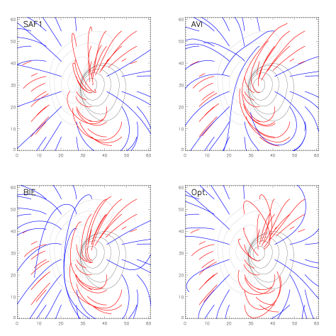
Fig. 1 : The magnetic field lines for each NLFF fields (SAF1, AVI, BIE and Opt. methods are labeled).

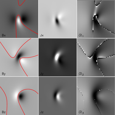
Fig. 2 : The images of $\alpha_{1}$, $\alpha_{2}$ and $\alpha_{3}$, the components of magnetic field and current ($J_{x}$, $J_{y}$, $J_{z}$) labeled in each frame for SAF1 at $z=0$.

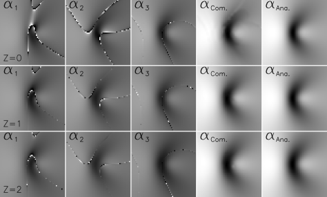
Fig. 3 : The images of $\alpha_{1}$, $\alpha_{2}$, $\alpha_{3}$, $\alpha_{Com.}$ and $\alpha_{Ana.}$ at $z=0$, $z=1$ and $z=2$ for SAF1. .

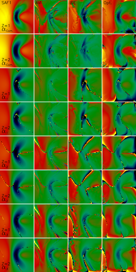
Fig. 4 : The images of $\alpha_{Com.,1,2,3}$ deduced from extrapolated fields at $z=1$ and $z=2$. (SAF1)

Fig. 5 : RSD ($\delta_{\alpha}$) of $\alpha_{Ana.}$ calculated from selected field lines for two semi-analytical fields (labeled).

Fig. 6 : The PDF of RSD ($\delta_{\alpha_{Com.,1,2,3}}$) calculated from some selected field lines for each NLFF field. (SAF1)

Fig. 7 : The scatter diagram of RSD ($\delta_{\alpha_{Com.,1,2,3}}$) vs the length of field line calculated from some selected field lines for each NLFF field. (SAF1)

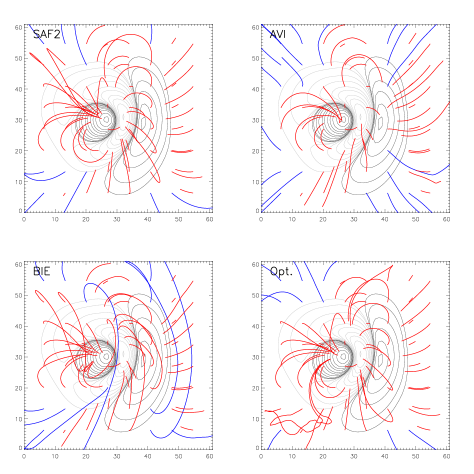
Fig. 8 : The magnetic field lines for each NLFF fields (SAF2, AVI, BIE and Opt. methods are labeled)

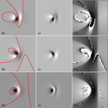
Fig. 9 : The images of $\alpha_{1}$, $\alpha_{2}$ and $\alpha_{3}$, the components of magnetic field and current ($J_{x}$, $J_{y}$, $J_{z}$) labeled in each frame for SAF2 at $z=0$.

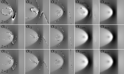
Fig. 10 : The images of $\alpha_{1}$, $\alpha_{1}$ and $\alpha_{1}$, $\alpha_{Com.}$ and $\alpha_{Ana.}$ at $z=0$, $z=1$ and $z=2$ for SAF2.

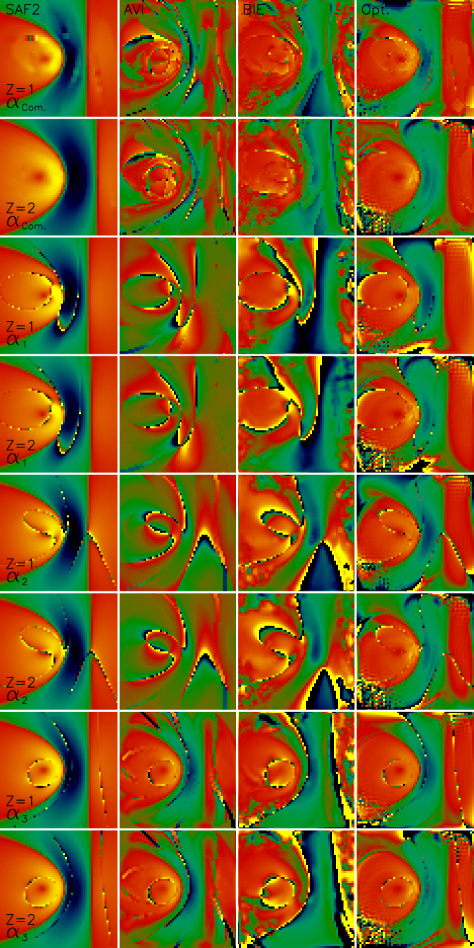
Fig. 11 : The images of $\alpha_{Com.,1,2,3}$ deduced from extrapolated fields at $z=1$ and $z=2$. (SAF2)

Fig. 12 : The PDF of RSD ($\delta_{\alpha_{Com.,1,2,3}}$) calculated from some selected field lines for each NLFF field. (SAF2)

Fig. 13 : The scatter diagram of RSD ($\delta_{\alpha_{Com.,1,2,3}}$) vs the length of field line calculated from some selected field lines for each NLFF field. (SAF2)

References

- Aly (1989) Aly, J.J.: 1989, Sol. Phys. 120, 19.
- Amari et al. (1997) Amari, T., Aly, J.J., Luciani, J.F., Boulmezaoud, T.Z., Mikic, Z.: 1997, Sol. Phys. 174, 129.
- Amari et al. (2006) Amari, T., Boulmezaoud, T.Z., Aly, J.J.: 2006, Astron. Astrophys. 446, 691.
- Chodura and Schlueter (1981) Chodura, R., Schlueter, A.: 1981, J. Chem. Phys. 41, 68.
- Cuperman et al. (1990) Cuperman, S., Ofman, L., Semel, M.: 1990, Astron. Astrophys. 230, 193.
- Démoulin et al. (1992) Démoulin, P., Cuperman, S., Semel, M.: 1992, Astron. Astrophys. 236, 351.
- DeRosa et al. (2009) DeRosa, M.L., Schrijver, C.J., Barnes, G., Leka, K.D., Lites, B.W., Aschwanden, M.J., et al.: 2009, Astrophys. J. 696, 1780
- He and Wang (2008) He, H., Wang, H.: 2008, J. Geophys. Res. 113, A05S90
- He et al. (2011) He, H., Wang, H.,Yan, Y.: 2011, J. Geophys. Res. 116, A01101
- Liu et al. (2011) Liu, S., Zhang, H.Q., Su, J.T. and Song, M.T.: 2011, Sol. Phys. 269, 41
- Li, Yan, and Song (2004) Li, Z, Yan, Y.H., Song, G.: 2004, Mon. Not. R. Astron. Soc. 347, 1255
- Low and Lou (1990) Low, B.C., Lou, Y.Q.: 1990, Astrophys. J. 352, 343
- Mikic and McClymont (1994) Mikic, Z.; McClymont, A. N.: 1994, in Solar Active Region Evolution: Comparing Models with Observations, Vol68. ASP Conf. Ser., p.225.
- Régnier et al. (2004) Régnier, S., Amari, T.: 2004, Astron. Astrophys. 425, 345.
- Régnier et al. (2007) Régnier, S., Priest, E. R.: 2007, Astron. Astrophys. 468, 701.
- Roumeliotis (1996) Roumeliotis, G.: 1996, Astrophys. J. 473, 1095
- Sakurai (1981) Sakurai, T.: 1981, Sol. Phys. 69, 343.
- Schrijver et al. (2006) Schrijver, C.J., De Rosa, M. L., Metcalf, T. R., Liu, Y., McTiernan, J., Régnier, S., Valori, G., Wheatland, M. S., Wiegelmann, T.: 2006, Sol. Phys. 235, 161.
- Song et al. (2006) Song, M.T., Fang, C., Tang, Y.H., Wu, S.T., Zhang, Y.A.: 2006, Astrophys. J. 649, 1084.
- Valori et al. (2007) Valori, G., Kliem, B., Fuhrmann, M.: 2007, Sol. Phys. 245, 263.
- Wheatland et al. (2000) Wheatland, M.S., Sturrock, P.A., Roumeliotis, G.: 2000, Astrophys. J. 540, 1150.
- Wiegelmann (2004) Wiegelmann, T.: 2004, Sol. Phys. 219, 87.
- Wiegelmann et al. (2006) Wiegelmann, T., Inhester, B., Sakurai, T.: 2006, Sol. Phys. 233, 215
- Wu et al. (1990) Wu, S.T., Sun, M.T., Chang, H.M., Hagyard, M.J., Gary, G.A.: 1990, Astrophys. J. 362, 698.
- Yan and Li (2006) Yan, Y., Li, Z.: 2006, Astrophys. J. 638, 1162.
- Yan and Sakurai (2000) Yan, Y., Sakurai, T.: 2000, Sol. Phys. 195, 89.