Volumes and Tangent Cones of Matroid Polytopes

Abstract.

De Loera et al. 2009, showed that when the rank is fixed the Ehrhart polynomial of a matroid polytope can be computed in polynomial time when the number of elements varies. A key to proving this is the fact that the number of simplicial cones in any triangulation of a tangent cone is bounded polynomially in the number of elements when the rank is fixed. The authors speculated whether or not the Ehrhart polynomial could be computed in polynomial time in terms of the number of bases, where the number of elements and rank are allowed to vary. We show here that for the uniform matroid of rank $r$ on $n$ elements, the number of simplicial cones in any triangulation of a tangent cone is $n-2\choose r-1$. Therefore, if the rank is allowed to vary, the number of simplicial cones grows exponentially in $n$. Thus, it is unlikely that a Brion-Lawrence type of approach, such as Barvinok’s Algorithm, can compute the Ehrhart polynomial efficiently when the rank varies with the number of elements. To prove this result, we provide a triangulation in which the maximal simplicies are in bijection with the spanning thrackles of the complete bipartite graph $K_{r,n-r}$.

1. Introduction

Recall that a matroid $M$ is a finite collection $\mathcal{F}$ of subsets of $[n]=\{1,2,\dots,n\}$ called independent sets, such that the following properties are satisfied: (1) $\emptyset\in\mathcal{F}$, (2) if $X\in\mathcal{F}$ and $Y\subseteq X$ then $Y\in\mathcal{F}$, (3) if $U,V\in\mathcal{F}$ and $|U|=|V|+1$ there exists $x\in U\setminus V$ such that $V\cup x\in\mathcal{F}$. In this paper we investigate convex polyhedra associated with matroids.

Similarly, recall that a matroid $M$ can be defined by its bases, which are the inclusion-maximal independent sets. The bases of a matroid $M$ can be recovered by its rank function $\varphi$. For the reader we recommend [6] or [11] for excellent introductions to the theory of matroids.

Now we introduce the main object of this paper. Let $\mathcal{B}$ be the set of bases of a matroid $M$. If $B=\{\sigma_{1},\ldots,\sigma_{r}\}\in\mathcal{B}$, we define the incidence vector of B as $\mathchoice{\mbox{\boldmath$\displaystyle\bf e$}}{\mbox{\boldmath$\textstyle\bf e$}}{\mbox{\boldmath$\scriptstyle\bf e$}}{\mbox{\boldmath$\scriptscriptstyle\bf e$}}_{B}:=\sum_{i=1}^{r}\mathchoice{\mbox{\boldmath$\displaystyle\bf e$}}{\mbox{\boldmath$\textstyle\bf e$}}{\mbox{\boldmath$\scriptstyle\bf e$}}{\mbox{\boldmath$\scriptscriptstyle\bf e$}}_{\sigma_{i}}$, where $\mathchoice{\mbox{\boldmath$\displaystyle\bf e$}}{\mbox{\boldmath$\textstyle\bf e$}}{\mbox{\boldmath$\scriptstyle\bf e$}}{\mbox{\boldmath$\scriptscriptstyle\bf e$}}_{j}$ is the standard elementary $j$th vector in $\mathbb{R}^{n}$. The matroid polytope of $M$ is defined as $\mathcal{P}(M):=\operatorname{conv}\{\,\mathchoice{\mbox{\boldmath$\displaystyle\bf e$}}{\mbox{\boldmath$\textstyle\bf e$}}{\mbox{\boldmath$\scriptstyle\bf e$}}{\mbox{\boldmath$\scriptscriptstyle\bf e$}}_{B}\mid B\in\mathcal{B}\,\}$, where $\operatorname{conv}(\cdot)$ denotes the convex hull. This is different from the well-known independence matroid polytope, $\mathcal{P}^{\mathcal{I}}(M):=\operatorname{conv}\{\,\mathchoice{\mbox{\boldmath$\displaystyle\bf e$}}{\mbox{\boldmath$\textstyle\bf e$}}{\mbox{\boldmath$\scriptstyle\bf e$}}{\mbox{\boldmath$\scriptscriptstyle\bf e$}}_{I}\mid I\subseteq B\in\mathcal{B}\,\}$, the convex hull of the incidence vectors of all the independent sets. We can see that $\mathcal{P}(M)\subseteq\mathcal{P}^{\mathcal{I}}(M)$ and $\mathcal{P}(M)$ is a face of $\mathcal{P}^{\mathcal{I}}(M)$ lying in the hyperplane $\sum_{i=1}^{n}x_{i}=\operatorname{rank}(M)$, where $\operatorname{rank}(M)$ is the cardinality of any basis of $M$.

Recall that given an integer $k>0$ and a polytope $\mathcal{P}\subseteq\mathbb{R}^{n}$ we define $k\mathcal{P}:=\{\,k\mathchoice{\mbox{\boldmath$\displaystyle\bf\alpha$}}{\mbox{\boldmath$\textstyle\bf\alpha$}}{\mbox{\boldmath$\scriptstyle\bf\alpha$}}{\mbox{\boldmath$\scriptscriptstyle\bf\alpha$}}\mid\mathchoice{\mbox{\boldmath$\displaystyle\bf\alpha$}}{\mbox{\boldmath$\textstyle\bf\alpha$}}{\mbox{\boldmath$\scriptstyle\bf\alpha$}}{\mbox{\boldmath$\scriptscriptstyle\bf\alpha$}}\in\mathcal{P}\,\}$ and the function $i(\mathcal{P},k):=\#(k\mathcal{P}\cap\mathbb{Z}^{n})$, where we define $i(\mathcal{P},0):=1$. It is well known that for integral polytopes, as in the case of matroid polytopes, $i(\mathcal{P},k)$ is a polynomial, called the Ehrhart polynomial of $\mathcal{P}$. Moreover the leading coefficient of the Ehrhart polynomial is the normalized volume of $\mathcal{P}$, where a unit is the volume of the fundamental domain of the affine lattice spanned by $\mathcal{P}$ [7]. In [2] the following was shown:

Theorem 1 ( Theorem 1 in [2]).

Let $r$ be a fixed integer. Then there exist algorithms whose input data consists of a number $n$ and an evaluation oracle for

1. a rank function $\varphi$ of a matroid $M$ on $n$ elements satisfying $\varphi(A)\leq r$ for all $A$, or

2. an integral polymatroid rank function $\psi$ satisfying $\psi(A)\leq r$ for all $A$,

that compute in time polynomial in $n$ the Ehrhart polynomial (in particular, the volume) of the matroid polytope $\mathcal{P}(M)$, the independence matroid polytope $\mathcal{P}^{\mathcal{I}}(M)$, and the polymatroid $\mathcal{P}(\psi)$, respectively.

The proof of Theorem 1 relied on four important facts when the rank is fixed: (1) The number of bases is polynomially bounded, (2) every triangulation of a tangent cone of the matroid polytope has a polynomial number of maximal simplicial cones, (3) a triangulation of a tangent cone can be done in polynomial time, and (4) every triangulation of a tangent cone of the matroid polytope is unimodular. The first item follows easily from the rank being fixed, implying there are at most $n\choose r$ bases. The third item is relatively straightforward using the pulling triangulation, given item two holds. The proof of item two in [2] (Lemma 10) used a bound on the volume of the subpolytope given by a vertex and all its adjacent vertices. Item four does not rely on the rank being fixed at all.

The authors of [2] speculated whether or not the Ehrhart polynomial of a matroid polytope could be computed in polynomial time with respect to the number of basis, regardless of the rank. The primary limitation to proving this result seemed to be item two above. However, we show the following:

Theorem 2.

Let $U^{r,n}$ be the uniform matroid of rank $r$ with $n$ elements. There are $n-2\choose r-1$ simplicial cones in any triangulation of a tangent cone of the matroid base polytope of $U^{r,n}$.

Thus, it is unlikely that the Erhrart polynomial of a matroid base polytope can be computed in polynomial time when the number of ground elements $n$ varies and the rank is not fixed. That is, a Brion-Lawrence type of approach (Barvinok’s Algorithm [1]) to compute the Ehrhart polynomial is likely not computationally efficient. If the rank is allowed to vary, Theorem 2 states that the number of simplicial cones in the triangulation of any tangent cone of $U^{n/2,n}$, where $n$ even, is $n-2\choose n/2-1$, the central binomial coefficient. And, it is known that $n-2\choose n/2-1$ grows exponentially in $n$.

2. Gröbner Bases and Triangulations

Notation and ideas for many of the proofs in this section are taken from [9] (which is in turn was drawn from [5]), which covers Gröbner bases and triangulations.

The edges of the matroid polytope have the following important property.

Lemma 2 (See Theorem 4.1 in [3], Theorem 5.1 and Corollary 5.5 in [10]).

Let $M$ be a matroid.

• Two vertices $\mathchoice{\mbox{\boldmath$\displaystyle\bf e$}}{\mbox{\boldmath$\textstyle\bf e$}}{\mbox{\boldmath$\scriptstyle\bf e$}}{\mbox{\boldmath$\scriptscriptstyle\bf e$}}_{B_{1}}$ and $\mathchoice{\mbox{\boldmath$\displaystyle\bf e$}}{\mbox{\boldmath$\textstyle\bf e$}}{\mbox{\boldmath$\scriptstyle\bf e$}}{\mbox{\boldmath$\scriptscriptstyle\bf e$}}_{B_{2}}$ are adjacent in $\mathcal{P}(M)$ if and only if $\mathchoice{\mbox{\boldmath$\displaystyle\bf e$}}{\mbox{\boldmath$\textstyle\bf e$}}{\mbox{\boldmath$\scriptstyle\bf e$}}{\mbox{\boldmath$\scriptscriptstyle\bf e$}}_{B_{1}}-\mathchoice{\mbox{\boldmath$\displaystyle\bf e$}}{\mbox{\boldmath$\textstyle\bf e$}}{\mbox{\boldmath$\scriptstyle\bf e$}}{\mbox{\boldmath$\scriptscriptstyle\bf e$}}_{B_{2}}=\mathchoice{\mbox{\boldmath$\displaystyle\bf e$}}{\mbox{\boldmath$\textstyle\bf e$}}{\mbox{\boldmath$\scriptstyle\bf e$}}{\mbox{\boldmath$\scriptscriptstyle\bf e$}}_{i}-\mathchoice{\mbox{\boldmath$\displaystyle\bf e$}}{\mbox{\boldmath$\textstyle\bf e$}}{\mbox{\boldmath$\scriptstyle\bf e$}}{\mbox{\boldmath$\scriptscriptstyle\bf e$}}_{j}$ for some $i,j$.

• If two vertices $\mathchoice{\mbox{\boldmath$\displaystyle\bf e$}}{\mbox{\boldmath$\textstyle\bf e$}}{\mbox{\boldmath$\scriptstyle\bf e$}}{\mbox{\boldmath$\scriptscriptstyle\bf e$}}_{I_{1}}$ and $\mathchoice{\mbox{\boldmath$\displaystyle\bf e$}}{\mbox{\boldmath$\textstyle\bf e$}}{\mbox{\boldmath$\scriptstyle\bf e$}}{\mbox{\boldmath$\scriptscriptstyle\bf e$}}_{I_{2}}$ are adjacent in $\mathcal{P}^{\mathcal{I}}(M)$ then $\mathchoice{\mbox{\boldmath$\displaystyle\bf e$}}{\mbox{\boldmath$\textstyle\bf e$}}{\mbox{\boldmath$\scriptstyle\bf e$}}{\mbox{\boldmath$\scriptscriptstyle\bf e$}}_{I_{1}}-\mathchoice{\mbox{\boldmath$\displaystyle\bf e$}}{\mbox{\boldmath$\textstyle\bf e$}}{\mbox{\boldmath$\scriptstyle\bf e$}}{\mbox{\boldmath$\scriptscriptstyle\bf e$}}_{I_{2}}\in\{\,\mathchoice{\mbox{\boldmath$\displaystyle\bf e$}}{\mbox{\boldmath$\textstyle\bf e$}}{\mbox{\boldmath$\scriptstyle\bf e$}}{\mbox{\boldmath$\scriptscriptstyle\bf e$}}_{i}-\mathchoice{\mbox{\boldmath$\displaystyle\bf e$}}{\mbox{\boldmath$\textstyle\bf e$}}{\mbox{\boldmath$\scriptstyle\bf e$}}{\mbox{\boldmath$\scriptscriptstyle\bf e$}}_{j},\,\mathchoice{\mbox{\boldmath$\displaystyle\bf e$}}{\mbox{\boldmath$\textstyle\bf e$}}{\mbox{\boldmath$\scriptstyle\bf e$}}{\mbox{\boldmath$\scriptscriptstyle\bf e$}}_{i},\,-\mathchoice{\mbox{\boldmath$\displaystyle\bf e$}}{\mbox{\boldmath$\textstyle\bf e$}}{\mbox{\boldmath$\scriptstyle\bf e$}}{\mbox{\boldmath$\scriptscriptstyle\bf e$}}_{j}\,\}$ for some $i,j$. Moreover if $\textstyle\bf v$ is a vertex of $\mathcal{P}^{\mathcal{I}}(M)$ then all adjacent vertices of $\textstyle\bf v$ can be computed in polynomial time in $n$, even if the matroid $M$ is only presented by an evaluation oracle of its rank function $\varphi$.

In this section we study the matroid polytopes of uniform matroids. Let $U^{r,n}$ denote the uniform matroid of rank $r$ on $n$ elements. If $B$ is a basis of $U^{r,n}$, then $B\backslash\{i\}\cup\{j\}$ is an adjacent basis on $\mathcal{P}(U^{r,n})$, for all $i\in B$ and $j\in[n]\backslash B$. Since we study the uniform matroid, without loss of generality, we focus on the basis $B=\{1,\ldots,r\}$ with incidence vector

$$[\underbrace{1,\ldots,1}_{r},\underbrace{0,\ldots,0}_{n-r}].$$

The bases adjacent to $B$ are then $\{1,\ldots,r\}\backslash\{i\}\cup\{j\}$ where $1\leq i\leq r$ and $r+1\leq j\leq n$. Shifting by the vector $\mathchoice{\mbox{\boldmath$\displaystyle\bf e$}}{\mbox{\boldmath$\textstyle\bf e$}}{\mbox{\boldmath$\scriptstyle\bf e$}}{\mbox{\boldmath$\scriptscriptstyle\bf e$}}_{B}$, we are interested in the pointed cone $C$ with rays $\mathchoice{\mbox{\boldmath$\displaystyle\bf e$}}{\mbox{\boldmath$\textstyle\bf e$}}{\mbox{\boldmath$\scriptstyle\bf e$}}{\mbox{\boldmath$\scriptscriptstyle\bf e$}}_{i}-\mathchoice{\mbox{\boldmath$\displaystyle\bf e$}}{\mbox{\boldmath$\textstyle\bf e$}}{\mbox{\boldmath$\scriptstyle\bf e$}}{\mbox{\boldmath$\scriptscriptstyle\bf e$}}_{j}$, for all $1\leq i\leq r$ and $r+1\leq j\leq n$. We define

$$\mathcal{E}_{r,n}:=\{\,\mathchoice{\mbox{\boldmath$\displaystyle\bf e$}}{\mbox{\boldmath$\textstyle\bf e$}}{\mbox{\boldmath$\scriptstyle\bf e$}}{\mbox{\boldmath$\scriptscriptstyle\bf e$}}_{j}-\mathchoice{\mbox{\boldmath$\displaystyle\bf e$}}{\mbox{\boldmath$\textstyle\bf e$}}{\mbox{\boldmath$\scriptstyle\bf e$}}{\mbox{\boldmath$\scriptscriptstyle\bf e$}}_{i}\mid 1\leq i\leq r,\,r+1\leq j\leq n\,\}.$$

Note that the points $\mathcal{E}_{r,n}$ lie in the hyperplane $[\underbrace{1,\ldots,1}_{r},\underbrace{-1,\ldots,-1}_{n-r}]\cdot\mathchoice{\mbox{\boldmath$\displaystyle\bf x$}}{\mbox{\boldmath$\textstyle\bf x$}}{\mbox{\boldmath$\scriptstyle\bf x$}}{\mbox{\boldmath$\scriptscriptstyle\bf x$}}=0$, which does not contain the origin. We are interested in triangulations of $C$ into simplicial cones. Note that any triangulation of $C$ is in bijection with triangulations of the points $\mathcal{E}_{r,n}$. Hence, we study triangulations of $\mathcal{E}_{r,n}$. To simplify matters and better relate to material in [9] we will focus on triangulations of

$$\mathcal{B}_{r,n}:=\{\,\mathchoice{\mbox{\boldmath$\displaystyle\bf e$}}{\mbox{\boldmath$\textstyle\bf e$}}{\mbox{\boldmath$\scriptstyle\bf e$}}{\mbox{\boldmath$\scriptscriptstyle\bf e$}}_{i}+\mathchoice{\mbox{\boldmath$\displaystyle\bf e$}}{\mbox{\boldmath$\textstyle\bf e$}}{\mbox{\boldmath$\scriptstyle\bf e$}}{\mbox{\boldmath$\scriptscriptstyle\bf e$}}_{j}\mid 1\leq i\leq r,\,r+1\leq j\leq n\,\}.$$

Note that $\operatorname{conv}(\mathcal{E}_{r,n})$ can be mapped to $\operatorname{conv}(\mathcal{B}_{r,n})$ by the unimodular involution

$$\left(\begin{array}[]{cc}-I_{r}&0\\ 0&I_{n-r}\end{array}\right).$$

Therefore triangulations of $\operatorname{conv}(\mathcal{E}_{r,n})$ and $\operatorname{conv}(\mathcal{B}_{r,n})$ are in bijection and their volumes are equal. Note that $\mathcal{B}_{r,n}$ is a sub-polytope of the second hypersimplex

$$\mathcal{A}_{n}:=\{\,\mathchoice{\mbox{\boldmath$\displaystyle\bf e$}}{\mbox{\boldmath$\textstyle\bf e$}}{\mbox{\boldmath$\scriptstyle\bf e$}}{\mbox{\boldmath$\scriptscriptstyle\bf e$}}_{i}+\mathchoice{\mbox{\boldmath$\displaystyle\bf e$}}{\mbox{\boldmath$\textstyle\bf e$}}{\mbox{\boldmath$\scriptstyle\bf e$}}{\mbox{\boldmath$\scriptscriptstyle\bf e$}}_{j}\mid 1\leq i<j\leq n\,\}.$$

We now follow closely the notation and proofs of Chapter 9 of [9]. In it, Sturmfels gives a unimodular triangulation of $\mathcal{A}_{n}$ into $2^{n-1}-n$ simplices.

Proposition 2.

The dimension of $\operatorname{conv}(\mathcal{B}_{r,n})$ is $n-2$.

Proof.

The points $\mathcal{B}_{r,n}$ lie in the hyperplanes $[1,\ldots,1]\cdot\mathchoice{\mbox{\boldmath$\displaystyle\bf x$}}{\mbox{\boldmath$\textstyle\bf x$}}{\mbox{\boldmath$\scriptstyle\bf x$}}{\mbox{\boldmath$\scriptscriptstyle\bf x$}}=2$ and $[\underbrace{1,\ldots,1}_{r},\underbrace{-1,\ldots,-1}_{n-r}]\cdot\mathchoice{\mbox{\boldmath$\displaystyle\bf x$}}{\mbox{\boldmath$\textstyle\bf x$}}{\mbox{\boldmath$\scriptstyle\bf x$}}{\mbox{\boldmath$\scriptscriptstyle\bf x$}}=0$. It is not difficult to see there are $n-2$ linearly independent vectors in $\mathcal{B}_{r,n}$. ∎

Remark 2.

The set of column vectors $\mathcal{B}_{r,n}$ is the vertex-edge incidence matrix of the complete bipartite graph $K_{r,n-r}$.

The toric ideal $I_{\mathcal{B}_{r,n}}$ is the kernel of the map

$$\Phi:k[x_{ij}\,:\,1\leq i\leq r,\,r+1\leq j\leq n]\rightarrow k[t_{1},\ldots,t_{n}],\,x_{ij}\mapsto t_{i}t_{j}.$$

The variables $x_{ij}$ are indexed by the edges of the complete bipartite graph $K_{r,n-r}$. We identify the vertices of $K_{r,n-r}$ with the vertices of a planar embedding of the complete bipartite graph on $r$ and $n-r$ vertices. By an edge we mean a closed line segment between two vertices in the complete bipartite graph on $r$ and $n-r$ vertices. The weight of the variable $x_{ij}$ is the number of edges of $K_{r,n-r}$ which do not meet the edge $(i,j)$.

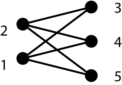
Figure 1. Complete bipartite graph $K_{2,3}$.

Example 2.

For $K_{2,3}$ in Figure 1, variables $x_{13},x_{25}$ have weight $0$, variable $x_{14},x_{24}$ have weight $1$, and variables $x_{15},x_{23}$ have weight $2$.

Remark 2.

Throughout this section, we will draw the complete bipartite graph $K_{s,t}$ as in Figure 1: The $s$ vertices $\{1,\ldots,s\}$ are drawn vertically on the left and labeled from bottom to top and the $t$ vertices $\{s+1,\ldots,s+t\}$ are drawn vertically on the right and labeled from top to bottom. This is done to match closely with [9], where the complete graphs $K_{n}$ are drawn on the $n$-gon with labels in clockwise order. Thus, for the drawings of the complete bipartite graph $K_{s,t}$ we can also talk about the $(s+t)$-gon given by the $s+t$ points.

Given any pair of non-intersecting edges $(i,j),(k,l)$ of $K_{r,n-r}$ the pair $(i,l),(j,k)$ meets in a point (intersect). With disjoint edges $(i,j),(k,l)$ we associate the binomial $x_{ij}x_{kl}-x_{il}x_{jk}$. We denote by $\mathcal{C}$ the set of all binomials obtained in this fashion, and by $in_{\succ}(\mathcal{C})$ the set of their initial monomials. Here $\succ$ denotes the term order that refines the partial order on monomials specified by these weights.

Example 2.

Let $r=2$, $n=5$. Then $\mathcal{C}$ is

$$\big{\{}\,\underline{x_{13}x_{25}}-x_{15}x_{23},\underline{x_{13}x_{24}}-x_{14}x_{23},\underline{x_{14}x_{25}}-x_{15}x_{24}\big{\}}.$$

Theorem 3.

The set $\mathcal{C}$ is the reduced Gröbner basis of $I_{B_{r,n}}$ with respect to $\succ$.

The proof of Theorem 3 follows nearly verbatim of the proof of Theorem 9.1 in [9], with only minor modification to handle the complete bipartite graph. The proof of Theorem 3 is given in the Appendix.

Remark 3 (Remark 9.2 in [9]).

The set $\mathcal{C}$ is the reduced Gröbner basis for $I_{B_{r,n}}$ with respect to the purely lexicigraphic term order induced by the following variable ordering:

$$x_{ij}\succ x_{kl}\quad\text{if and only if}\quad i<k\text{ or }(i=k\text{ and }j>l).$$

Proof.

For any ordered quadruple $1\leq i<j<k<l\leq n$, the intersecting pair of edges is $\{(i,k),(j,l)\}$. We must show that the monomial $x_{ik}x_{jl}$ is smaller than both $x_{ij}x_{jk}$ in the given term order. But this holds since $x_{kl}\succ x_{jk}\succ x_{jl}\succ x_{ij}\succ x_{ik}\succ x_{il}$. ∎

Following identical logic in Chaption 9 of [9], we apply Theorem 3 to give an explicit triangulation and determine the normalized volume of $\operatorname{conv}(B_{r,n})$. By Theorem 8.3 in [9], the square-free monomial ideal $\langle\operatorname{in}_{\succ}(\mathcal{C})\rangle=in_{\succ}(I_{B_{r,n}})$ is the Stanley-Reisner ideal of a regular triangulation $\Delta_{\succ}$ of $\operatorname{conv}(B_{r,n})$. The simplices in $\Delta_{\succ}$ are the supports of the standard monomials. All maximal simplicies in $\Delta_{\succ}$ have unit normalized volume by Corollary 8.9 in [9], Corollary 63 in [4], or Lemma 8 in [2]. We observed before that elements of $\operatorname{in}_{\succ}(\mathcal{C})$, the minimally non-standard monomials, are supported on pairs of disjoint edges.

Corollary 3.

The simplices of $\Delta_{\succ}$ are the subgraphs of $K_{r,n-r}$ with the property that any pair of edges intersects in the convex embedding of the graph given in 2.

Now we identify subgraphs of $K_{r,n-r}$ with subpolytopes of $\operatorname{conv}(B_{r,n})$: A subgraph $H$ is identified with the convex hull of the column vectors of its vertex-edge incidence matrix.

Definition 3.

Let $G$ be a graph with edge set $E$ embedded in the plane. Recall the edges $\widehat{E}\subseteq E$ are a thrackle if every pair of edges intersects.

Proposition 3.

A subpolytope $\sigma$ of $\operatorname{conv}(B_{r,n})$ is a $(n-2)$-dimensional simplex if and only if the coresponding subgraph $H$ is a spanning tree of $K_{r,n-r}$. The normalized volume of $\sigma$ is $1$.

Proof.

Suppose $H$ supports a $(n-2)$-simplex. Let $M_{H}$ be the $\{0,1\}$-incidence matrix of $H$. This matrix is non-singular which implies it is spanning and all cycles are odd (if any). But, the complete bipartite graph does not have odd cycles. Therefore $H$ is acyclic and spanning. Any acyclic spanning subgraph of $K_{r,n-r}$ with $n-1$ edges is a spanning tree.

Conversely, if $H$ is a spanning tree of $K_{r,n-r}$, it contains $n-1$ edges, is acyclic and its incidence matrix is non-singular implying it is a $(d-2)$-simplex.

There exists some vertex $v\in[n]$ such that the degree of $v$ is $1$. Performing cofactor expansion on the $v$th row we see that $M_{H}=M_{H-v}$. Repeating we see that $|M_{H}|=1$. ∎

Theorem 4.

The maximal simplices of the triangulation $\Delta_{\succ}$ are the spanning trees of $K_{r,n-r}$ with $n-1$ edges and with the property that any pair of edges intersects.

Proof.

Follows from 3 and 3. ∎

Proposition 4.

Every thrackle of $K_{s,t}$ is acyclic.

Proof.

All cycles in $K_{s,t}$ must be even, but as shown in the proof of Theorem 3, any even cycle will contain two edges that do not cross. ∎

Theorem 4 states that the simplices of $\Delta_{\succ}$ are the spanning thrackles of $K_{r,n-r}$. It is known that the number of spanning trees of $K_{r,n-r}$ is $r^{n-r-1}n^{r-1}$, but from Lemma 10 in [2] and by observation, not all spanning trees are thrackles. Below we prove that the number of spanning thrackles is simply a binomial coefficient.

We first observe a basic fact about thrackles on $K_{r,n-r}$.

Proposition 4.

Let $K_{s,t}$ be the complete bipartite graph with the planar embedding in 2, $H$ a thrackle of $K_{s,t}$, $1\leq i\leq s$, $s+1\leq j_{1}<j_{2}\leq s+t$, $j_{1}+1<j_{2}$ and $\{(i,j_{1}),(i,j_{2})\}$ edges of $H$. Then for all $k\in[s]\backslash\{i\}$ and $j_{1}<l<j_{2}$, $(k,l)$ does not intersect every edge of $H$.

Proof.

Let $K_{s,t}$ be the complete bipartite graph with the planar embedding in 2, $H$ a thrackle of $K_{s,t}$, $1\leq i\leq s$, $s+1\leq j_{1}\leq j_{2}\leq s+t$, $j_{1}+1<j_{2}$ and $\{(i,j_{1}),(i,j_{2})\}$ edges of $H$. If $k>i$ then $(k,l)$ does not intersect $(i,j_{2})$. If $k<i$ then $(k,l)$ does not intersect $(i,j_{1})$. ∎

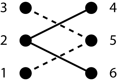
Figure 2. A thrackle (solid) with edges $\{(2,4),(2,6)\}$. No other edges (dashed) incident to vertex $5$ and not incident to vertex $2$ can be added to the thrackle to give a new thrackle.

For an example of 4, see Figure 2. From the above proposition we get the following corollary

Corollary 4.

Let $K_{s,t}$ be the complete bipartite graph with the planar embedding in 2. If $H$ is a spanning thrackle of $K_{s,t}$, $1\leq i\leq s$, $s+1\leq j_{1}\leq j_{2}\leq s+t$, $j_{1}+1<j_{2}$ and $\{(i,j_{1}),(i,j_{2})\}$ edges of $H$, then for all $j_{1}\leq j_{3}\leq j_{2}$, $(i,j_{3})$ is an edge of $H$.

Proposition 4.

Let $K_{s,t}$ be the complete bipartite graph with the planar embedding in 2 and $H$ a spanning thrackle of $K_{s,t}$. Then $\{1,s+1\}$ must be in $H$.

Proof.

Since $H$ is spanning, some edge of $H$ must be incident to $s+1$. But, this edge will not intersect any edge $\{1,j\}$ where $s+1<j\leq s+t$. ∎

Definition 4.

Let $K_{s,t}$ be the complete bipartite graph with the planar embedding in 2. We define $f(s,t)$ to be number of spanning thrackles of $K_{s,t}$.

By observation we see that $f(1,1)=1$ and $f(1,t)=1$ for all $1\leq t$. Also note that $f(s,t)=f(t,s)$.

Proposition 4.

Let $K_{s,t}$ be the complete bipartite graph with the planar embedding in 2. The number of spanning thrackles such that the only edges incident to vertex $1$ are $\{(1,s+1),\ldots,(1,i)\}$ where $s+1\leq i\leq t+s$ is $f(s-1,t+s+1-i))$.

Proof.

Let $K_{s,t}$ be the complete bipartite graph with the planar embedding in 2 and $H$ a spanning thrackle such that the only edges incident to vertex $1$ are $\{(1,s+1),\ldots,(1,i)\}$ where $s+1\leq i\leq t+s$. For any $1<j\leq s$ and $s+1\leq k<i$ we have that $(j,k)$ does not intersect the edges $\{(1,s+1),\ldots,(1,i)\}$. Therefore, the number of spanning thrackles such that the only edges incident to vertex $1$ are $\{(1,s+1),\ldots,(1,i)\}$ where $s+1\leq i\leq t+s$ equals $f(s-1,t+s+1-i))$. ∎

Using 4, we find a recurrence relation for the number of spanning thrackles of $K_{s,t}$ by dividing the spanning thrackles $H$ into disjoint cases (see Figure 3):

1. The only edge incident to $1$ is $\{(1,s+1)\}$.

2. The only edges incident to $1$ are $\{(1,s+1),(1,s+2)\}$.

3. The only edges incident to $1$ are $\{(1,s+1),(1,s+2),(1,s+3)\}$.
   $\vdots$

4. The only edges incident to $1$ are $\{(1,s+1),(1,s+2),\ldots,(1,s+t)\}$.

In item (1), if the only edge incident to $1$ in $H$ is $\{(1,s+1)\}$, then the number of spanning thrackles satisfying this condition is equal to $f(s-1,s+t)$. Similarly, if the only edges incident to $1$ in $H$ are $\{(1,s+1),(1,s+2)\}$, then the number of spanning thrackles satisfying this condition is equal to $f(s-1,s+t-1)$. This leads to the recursion relation

$$f(s,t)=\sum_{i=0}^{t-1}f(s-1,t-i).$$ (1)

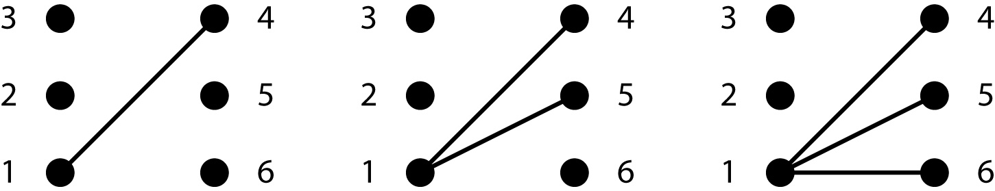
Figure 3. For $K_{3,3}$, the spanning thrackles fall into three disjoint cases. The only edge incident to $1$ is $(1,4)$ (left). The only edge incident to $1$ is $\{(1,4),(1,5)\}$ (middle). The only edge incident to $1$ is $\{(1,4),(1,5),(1,6)\}$ (right).

Lemma 4.

Let $K_{s,t}$ be the complete bipartite graph with the planar embedding in 2 and $H$ a spanning thrackle of $K_{s,t}$. The edges

$$\left\{\,(i,j)\in H\mid\nexists k,\,k<j,\,(i,k)\in H\,\right\}$$ (2)

uniquely determine $H$.

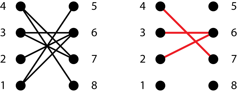
Figure 4. For the spanning thrackle (left) of $K_{4,4}$ the red edges (right) uniquely determine the thrackle.

See Figure 4 for an example.

Proof of 4.

By 4 and 4 the vertices incident to vertex $1$ must be an interval $[s+1,i_{1}]$ where $s+1\leq i_{1}\leq s+t$. Similarly, by the recursive argument in 4, the vertices incident to vertex $2$ must be an interval $[i_{1},i_{2}]$ where $i_{1}\leq i_{2}\leq s+t$. Continuing this argument, the vertices $1,2,\ldots,s$ are incident to the interval of vertices $[s+1,i_{1}],[i_{1},i_{2}],[i_{2},i_{3}],\ldots,[i_{s-1},s+t]$ respectively. Thus, $H$ is uniquely determined by $i_{1},\ldots,i_{s-1}$ and these are precisely what are given in Equation (2). ∎

Remark 4.

Note that if $(i,j)$ is an edge in the set 2, then for all $(k,l)$ in the set 2 such that $k>i$ we have $l\geq j$.

Recall from [8] that a weak composition of a positive integer $p$ is an ordered sum of $q$ non-negative integers which sums to $p$. It is known that the number of such weak composition is $p+q-1\choose q-1$.

Corollary 4.

The number of spanning thrackles $f(s,t)$ of the complete bipartite graph $K_{s,t}$ embedded in the plane as in 2 is equal to $s+t-2\choose s-1$. I.e.,

$$f(s,t)={s+t-2\choose s-1}={s+t-2\choose t-1}.$$ (3)

Proof.

4 states that the edges of Equation (2) uniquely determine the spanning thrackle. But, it can be seen that these edges are in bijection with the weak compositions of $t-1$ into $s$ parts. Hence Equation 3 holdes. ∎

Now we are equipped to prove Theorem 2.

Proof of Theorem 2.

By Theorem 4 the simplices of $\Delta_{\succ}$ are the maximal spanning thrackles, and from 4, we know this to be $n-2\choose r-1$. Now $\Delta_{\succ}$ is but one possible triangulation of the tangent cone. But, by Corollary 8.9 in [9], Corollary 63 in [4], or Lemma 8 in [2], we know that any triangulation of a tangent cone of a matroid polytope will be composed of unimodular cones. Hence it will have the same normalized volume, namely $n-2\choose r-1$. ∎

Finally, we offer an alternative method to prove Equation (3). We give a function $\Phi$ from the space spanning thrackles of $K_{s,t}$ embedded as in 2 to the space of $\{0,1\}$ sequences with exactly $s-1$ zeros and $t-1$ ones. Let $H$ be a spanning thrackle. The string $\Phi(H)$ is given by the algorithm:

Algorithm 4.

Input: A spanning thrackle $H$ of $K_{s,t}$ embedded as in 2. Output: A $\{0,1\}$ string with exactly $s-1$ zeros and $t-1$ ones. 1: Let $S$ = “”; 2: for every edge $v\in[s+1,s+t-1]$ do 3: for every vertex $w\neq 1$ adjacent to $v$ in $H$ and $w$ is unmarked do 4: S = S + “0”. 5: Mark $w$. 6: S = S + “1”. 7: for every vertex $w\neq 1$ adjacent to $s+t$ in $H$ and $w$ is unmarked do 8: S = S + “0”. 9: Mark $w$.

Following this, it is known the number of such $\{0,1\}$ strings is $s+t-2\choose s-1$. For an example of 4 (i.e. $\Phi$), see Figure 5.

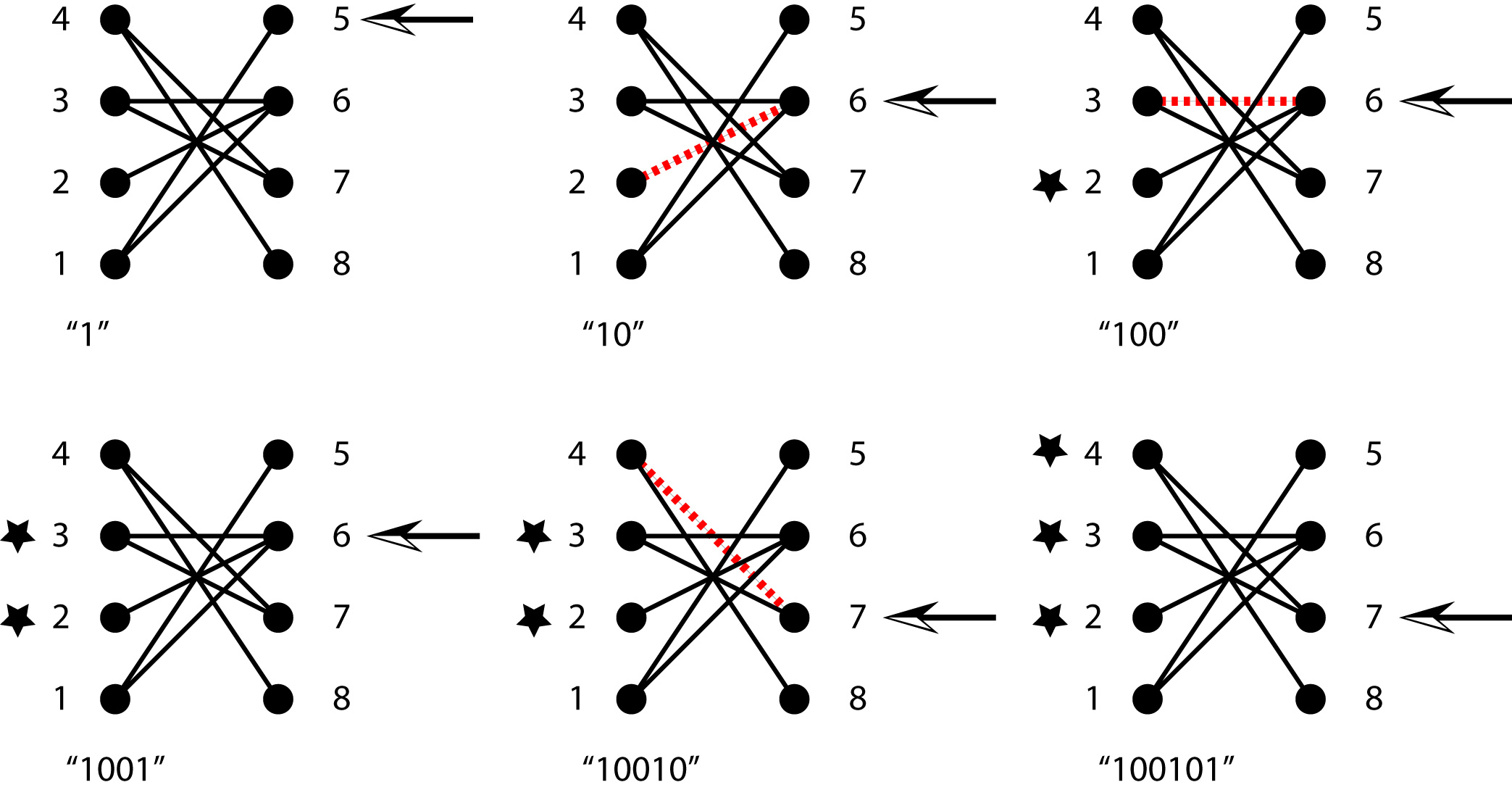
Figure 5. An example of 4 mapping of a spanning thrackle to a $\{0,1\}$ sequence with $s-1$ zeros and $t-1$ ones.

3. Discussion

If $M$ is not the uniform matroid, then the extreme rays of a tangent cone will not necessarily be $\mathcal{E}_{r,n}$. However, the arguments in Theorem 3 will still hold for any sub-polytope of $\operatorname{conv}(B_{r,n})$. In this case, instead of the complete bipartite graph $K_{r,n-r}$, we would have a subgraph $G$ of $K_{r,n-r}$. The maximal simplices of $\Delta_{\succ}$ would correspond to maximal thrackles of $G$. It would be interesting to study the number of such thrackles for other classes of matroids such as graphs, transversals, etc.

It should be noted that the volume of any tangent cone for any matroid of rank $r$ on $n$ elements is bounded by the volume of the tangent cone of the uniform matroid $U^{r,n}$. That is, bounded by $n-2\choose r-1$. Also immediate from Theorem 2 is that when the rank is fixed, the volume of the tangent cone is bounded polynomially in $n$. This provides an alternate proof of Lemma 10 in [2].

Unfortunately, knowledge of the exact volume of the convex hull of a vertex of a matroid polytope and its adjacent vertices does not immediately give a bound on the volume of the matroid polytope itself. There are points in the matroid polytope that are not in the convex hull of a vertex of a matroid polytope and its adjacent vertices.

4. appendix

Proof of Theorem 3.

Note the reduction relation defined by the proposed Gröbner basis amounts to replacing non-crossing edges by crossing edges. For each binomial $x_{ij}x_{kl}-x_{il}x_{jk}$ in $\mathcal{C}$, the initial term with respect to $\succ$ corresponds to the disjoint edges. This follows from the convex embedding of $K_{r,n-r}$ and the definition of the weights. The integral vectors in the kernel of $\mathcal{B}_{r,n}$ are in bijection with even length closed walks on th complete bipartite graph $K_{r,n-r}$, and hence so are the binomials of $I_{\mathcal{B}_{r,n}}$. More precisely, with an even walk $\Gamma=(i_{1},i_{2},\ldots,i_{2k-1},i_{2k},i_{1})$ we associate the binomial

$$b_{\Gamma}=\prod_{l=1}^{k}x_{i_{2l-1},i_{2l}}-\prod_{l=1}^{k}x_{i_{2l},i_{2l+1}}$$

where $i_{2k+1}=i_{1}$. Clearly the walk $\Gamma$ can be recovered from its binomial $b_{\Gamma}$. By Corollary 4.4 of [9], the infinite set of binomials associated with all even closed walks in $K_{r,n-r}$ contains every reduced Gröbner basis of $I_{\mathcal{B}_{r,n}}$. Therefore, in order to prove that $\mathcal{C}$ is a Gröbner basis, it is enough to prove that the initial monomial of any binomial $b_{\Gamma}$ is divisible by some monomial $x_{ij}x_{kl}$ where $(i,j),(k,l)$ is the pair of disjoint edges.

Suppose on the contrary there exists a binomial $b_{\Gamma}\in I_{\mathcal{B}_{r,n}}$ that contradicts our assertion. This implies that each pair of edges appearing in the initial monomial of $b_{\Gamma}$ intersects. We may assume that $b_{\Gamma}$ is a minimial counter-example in the sense that $r,n$ are minimal and $b_{\Gamma}$ has minimal weight. Hence the weight of the binomial $b_{\Gamma}$ is the sum of the weights of its two terms. The walk $\Gamma$ is spanning in $K_{r,n-r}$ by minimality of $n$. Every edge of $\Gamma$ gets a label ”odd” or ”even” according to its position on the walk. In the case of the complete bipartite graph, the odd edges go from $1\leq i\leq r$ to $r+1\leq j\leq n$, and even edges go in the opposite direction. If an edge is visited more than once, it can not receive both ”odd” and ”even”, since otherwise the related variable can be factored out of $b_{\Gamma}$. This would contradict the minimality of the weight. Alternatively, due to the fact above about odd and even edges on the bipartite graph, this will not occur. Moreover, if $b_{\Gamma}=\mathchoice{\mbox{\boldmath$\displaystyle\bf x$}}{\mbox{\boldmath$\textstyle\bf x$}}{\mbox{\boldmath$\scriptstyle\bf x$}}{\mbox{\boldmath$\scriptscriptstyle\bf x$}}^{\mathchoice{\mbox{\boldmath$\displaystyle\bf u$}}{\mbox{\boldmath$\textstyle\bf u$}}{\mbox{\boldmath$\scriptstyle\bf u$}}{\mbox{\boldmath$\scriptscriptstyle\bf u$}}}-\mathchoice{\mbox{\boldmath$\displaystyle\bf x$}}{\mbox{\boldmath$\textstyle\bf x$}}{\mbox{\boldmath$\scriptstyle\bf x$}}{\mbox{\boldmath$\scriptscriptstyle\bf x$}}^{\mathchoice{\mbox{\boldmath$\displaystyle\bf v$}}{\mbox{\boldmath$\textstyle\bf v$}}{\mbox{\boldmath$\scriptstyle\bf v$}}{\mbox{\boldmath$\scriptscriptstyle\bf v$}}}$ and $in_{\succ}(b_{\Gamma})=\mathchoice{\mbox{\boldmath$\displaystyle\bf x$}}{\mbox{\boldmath$\textstyle\bf x$}}{\mbox{\boldmath$\scriptstyle\bf x$}}{\mbox{\boldmath$\scriptscriptstyle\bf x$}}^{\mathchoice{\mbox{\boldmath$\displaystyle\bf u$}}{\mbox{\boldmath$\textstyle\bf u$}}{\mbox{\boldmath$\scriptstyle\bf u$}}{\mbox{\boldmath$\scriptscriptstyle\bf u$}}}$, we can assume that each pair of edges in $\mathchoice{\mbox{\boldmath$\displaystyle\bf x$}}{\mbox{\boldmath$\textstyle\bf x$}}{\mbox{\boldmath$\scriptstyle\bf x$}}{\mbox{\boldmath$\scriptscriptstyle\bf x$}}^{\mathchoice{\mbox{\boldmath$\displaystyle\bf v$}}{\mbox{\boldmath$\textstyle\bf v$}}{\mbox{\boldmath$\scriptstyle\bf v$}}{\mbox{\boldmath$\scriptscriptstyle\bf v$}}}$ intersects. Otherwise if $(i,j),(k,l)$ is a non-intersecting pair of edges then we can reduce $\mathchoice{\mbox{\boldmath$\displaystyle\bf x$}}{\mbox{\boldmath$\textstyle\bf x$}}{\mbox{\boldmath$\scriptstyle\bf x$}}{\mbox{\boldmath$\scriptscriptstyle\bf x$}}^{\mathchoice{\mbox{\boldmath$\displaystyle\bf v$}}{\mbox{\boldmath$\textstyle\bf v$}}{\mbox{\boldmath$\scriptstyle\bf v$}}{\mbox{\boldmath$\scriptscriptstyle\bf v$}}}$ modulo $\mathcal{C}$ to obtain a counterexample of smaller weight.

Suppose we draw $K_{r,n-r}$ as described in 2. The circular distance between any two vertices $1\leq i\leq r$ and $r+1\leq j\leq n$ is the shortest distance between $i$ and $j$ on the n-gon.

Let $(s,t)$ be an edge of the walk $\Gamma$ such that the circular distance between $s$ and $t$ is smallest possible. The edge $(s,t)$ separates the vertices of $K_{r,n-r}$, except $s$ and $t$, into two disjoint sets $P$ and $Q$ where $|P|\geq|Q|$. Let us assume the walk starts at $(s,t)=(i_{1},i_{2})$. The walk is then a sequence of vertices and edges $\Gamma=(i_{1},(i_{1},i_{2}),i_{2},(i_{2},i_{3}),\ldots,i_{2k},(i_{2k},i_{2k+1}))$. Each pair of odd (resp. even) edges intersects. The odd edges are of type $(i_{2r-1},i_{2r})$ and the even edges are of type $(i_{2r},i_{2r+1})$. Since the circular distance of $(i_{1},i_{2})$ is minimal, the vertex $i_{3}$ can not be in $Q$. Otherwise the edge $(i_{2},i_{3})$ would have smaller cicular distance. We claim that if $P$ contains an odd vertex $i_{2r-1}$, then it also contains the subsequent odd vertices $i_{2r+1},i_{2r+3},\ldots,i_{2k-1}$. The edge $(i_{1},i_{2})$ is the common boundary of the two regions $P$ and $Q$. Any odd edge intersects it (at least by having an end $\{i_{1},i_{2}\}$) and thus $i_{2r}$ is in $Q\cup\{i_{1},i_{2}\}$. Since any even edge must intersect $(i_{2},i_{3})$, the vertex $i_{2r+1}$ lies in $P\cup\{i_{2}\}$. To complete the proof of the claim we show that $i_{2r+1}\neq i_{2}$. The equality $i_{2r+1}=i_{2}$ would imply either $i_{2r}=i_{1}$ or $i_{2r}\in Q$. If $i_{2r}=i_{1}$ then $(i_{1},i_{2})$ is both odd and even. On the other hand if $i_{2r}\in Q$ then $(i_{2r},i_{2})$ has smaller circular distance than $(i_{1},i_{2})$. Thus $i_{2r+1}$ belongs to $P$. The claim is proved by repeating this argument.

Since $i_{3}$ was shown to be in $P$, it follows that all odd vertices except $i_{1}$ lie in $P$ and the even vertices lie in $Q\cup\{i_{1},i_{2}\}$. The final vertex $i_{2k}$ is thus in $Q$. The even edge $(i_{2k},i_{1})$ must be a closed line segment contained in the region $Q$. Therefore $(i_{1},i_{3})$ and $(i_{2k},i_{1})$ are two even edges that do not intersect, which is a contradiction. This proves $\mathcal{C}$ is a Gröbner basis of $I_{\mathcal{B}_{r,n}}$.

By construction, no monomial in an element of $\mathcal{C}$ is divisible by the initial term of an element in $\mathcal{C}$. Hence $\mathcal{C}$ is the reduced Gröbner basis of $I_{\mathcal{B}_{r,n}}$ with respect to $\succ$. ∎

References

- [1] Alexander I. Barvinok. Polynomial time algorithm for counting integral points in polyhedra when the dimension is fixed. Mathematics of Operations Research, 19:769–779, 1994.
- [2] Jesus A. De Loera, David Haws, and Matthias Köppe. Ehrhart polynomials of matroid polytopes and polymatroids. Journal of Discrete and Computational Geometry, 2009.
- [3] I. M. Gelfand, M. Goresky, R. D. MacPherson, and V. V. Serganova. Combinatorial geometries, convex polyhedra, and Schubert cells. Adv. Math., 63:301–316, 1987.
- [4] David Haws. Matroid polytopes: Algorithms, theory, and applications. arXiv:0905.4405, 2009.
- [5] J. De Loera, B. Sturmfels, and R. Thomas. Gröbner bases and triangulations of the second hypersimplex. Combinatorica, 15:409–424, 1995.
- [6] J. Oxley. Matroid Theory. Oxford University Press, New York, NY, USA, 1992.
- [7] Richard P. Stanley. Combinatorics and Commutative Algebra: Second Edition. Birkhäuser, Boston, 2nd edition, 1996.
- [8] Richard P. Stanley. Enumerative Combinatorics, volume 1. Cambridge University Press, 1997.
- [9] Bernd Sturmfels. Gröbner Bases and Convex Polytopes, volume 8 of University Lecture Series. American Mathematical Society, 1996.
- [10] D. M. Topkis. Adjacency on polymatroids. Mathematical Programming, 30(2):229–237, October 1984.
- [11] D. Welsh. Matroid Theory. Academic Press, Inc., 1976.