Comparison of $f$-vectors of Random Polytopes to the Gaussian Distribution

Abstract.

Choose $n$ random, independent points in $\mathbb{R}^{d}$ according to a fixed distribution. The convex hull of these points is a random polytope. In some cases, central limit theorems have been proven for the components of $f$-vectors of random polytopes constructed in this and similar ways. In this paper, we provide numerical evidence that the components of the $f$-vectors of random polytopes generated according to five different distributions are approximately jointly Gaussian for large $n$.

1. Introduction

Phenomena in high dimensions have been the subject of many studies. In particular, one may be interested in studying higher dimensional geometric objects called polytopes. A $polytope$ $P\in\mathbb{R}^{d}$ is a bounded subset of $\mathbb{R}^{d}$ formed by taking the intersection of finitely many halfspaces. The $f$-vector of a polytope $P$ is a vector $f=(f_{0},f_{1}...,f_{d-1})$ such that $f_{i}$ is the number of $i$-dimensional faces of $P$. In particular, $f_{0}$ is the number of vertices of $P$ and $f_{d-1}$ is the number of $(d-1)$-dimensional faces, known as $facets$.

There are some known results on the distribution of the $f$-vector of types of random polytopes. Previous work has found that individual components of the $f$-vectors are approximately Gaussian when the polytopes are generated according to various distributions. In particular, Bárány and Vu [3] proved that if a polytope is taken as the convex hull of independent and identically distributed (i.i.d.) points according to the standard Gaussian distribution, then the volume and individual components of the $f$-vector of that polytope satisfy a central limit theorem; that is, converge to a Gaussian distribution as the number of i.i.d. random points tends to infinity. Bárány and Reitzner [2] proved central limit theorems for the volume and components of the $f$-vector of a so-called Poisson random polytope; that is, the convex hull of the intersection of an arbitrary volume 1 convex body $K$ with a Poisson process $\chi$. Following earlier work of Reitzner [4], Vu [5] proved that the volume and components of the $f$-vector of a random polytope drawn from points inside a smooth convex set also satisfy central limit theorems.

In this paper, we consider the joint distributions of the $f$-vectors of random polytopes. The method used in this paper for constructing a random polytope is taking the convex hull of a set of i.i.d. random points generated from a fixed distribution. Our conjecture is the following:

1.1. Conjecture

Let N be a positive integer. Let $\mathcal{X}_{N}=\{X_{1},...,X_{n}\}$ be a collection of random points $X_{i}\in\mathbb{R}^{d}$, which are independent and identically distributed according to a fixed distribution. Letting $P_{N}\in\mathbb{R}^{d}$ be the convex hull of $\mathcal{X}_{N}$, under mild assumptions on the distribution of the $X_{i}$, the joint distribution of the $f$-vector satisifes a central limit theorem.

1.2. Results

In the five underlying distributions of the random points considered, numerical evidence supports the conjecture. The metric used to compare the closeness of the distribution of the $f$-vectors with the Gaussian distribution is based on the Kolmogorov distance, $D_{K}$. For now one may think of $D_{K}$ as a tool that measures the distance between two distributions and that $0\leq D_{K}\leq 1$. If $D_{K}$ is a small value then the two distributions are considered to be close to each other. The values of $D_{K}$ presented in the table are for comparison to the appropriate Gaussian distribution; details are discussed in section 3. Here, $d$ is the dimension, $n$ is the number of random points, and $N$ is the sample size or number of $f$-vectors.

Table 1. Uniform Distribution in Cube

$d$	$n$	$N$	$D_{K}$
5	64000	25000	0.	008995
6	64000	25000	0.	007590
7	8000	25000	0.	007133
8	1000	3125	0.	02613

Table 2. Uniform Distribution in $\ell_{1}$ Ball

$d$	$n$	$N$	$D_{K}$
5	64000	25000	0.	009971
6	64000	25000	0.	01075
7	4000	25000	0.	01113
8	1000	2000	0.	03003

Table 3. Uniform Distribution in $\ell_{2}$ Ball

$d$	$n$	$N$	$D_{K}$
5	64000	25000	0.	008495
6	64000	25000	0.	007873
7	2000	25000	0.	01182
8	1000	940	0.	04573

Table 4. Standard Gaussian Distribution

$d$	$n$	$N$	$D_{K}$
5	64000	25000	0.	01197
6	64000	25000	0.	01125
7	64000	25000	0.	009252
8	32000	1000	0.	01530

Table 5. Uniform Distribution in Hemisphere

$d$	$n$	$N$	$D_{K}$
5	64000	25000	0.	006166
6	4000	25000	0.	008827
7	500	12500	0.	02883

Since $D_{K}$ is a metric that takes on values in the interval [0,1], a value with order of magnitude $10^{-3}$ as the Kolmogorov distance should be considered a rather small value.

Figure 1 contains histograms of individual components of 64,000 $f$-vectors computed from the convex hull of 25,000 i.i.d. random points uniformly distributed in the 5-dimensional cube. After standardizing the $f$-vectors to have sample mean zero and identity sample covariance, the resulting data lie in $\mathbb{R}^{2}$. As further illustration, the 2-dimensional data of the standardized $f$-vector is plotted in $\mathbb{R}^{3}$.

(a) $f_{0}$

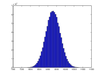
(b) $f_{1}$

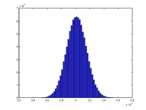
(c) $f_{2}$

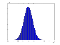
(d) $f_{3}$

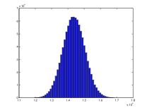
(e) $f_{4}$

Figure 1. Histograms of components of $f$-vectors in $\mathbb{R}^{5}$. Data came from 25,000 $f$-vectors computed from random polytopes generated by 64,000 i.i.d. uniformly distributed points in the 5-dimensional cube.

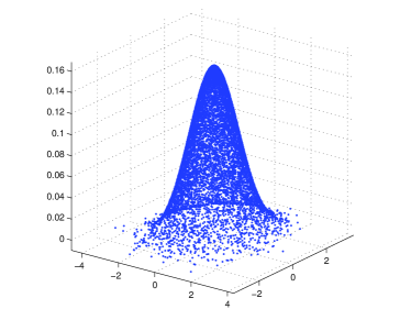
Figure 2. Standardized $f$-vectors in $\mathbb{R}^{5}$. Data came from 25,000 $f$-vectors computed from random polytopes generated by 64,000 i.i.d. uniformly distributed points in the 5-dimensional cube.

2. Background

It was mentioned in the introduction that one way to construct a random polytope is to take the convex hull of random points. One way to generate random points is to let $\{X_{i}\}_{i=1}^{n}$ be a collection of points generated independently according to a fixed distribution. Five distributions used to generate random points were considered and the random polytope studied was the convex hull of the $\{X_{i}\}_{i=1}^{n}$. The underlying distributions considered are the following:

1. Uniform in the Cube. Define $B_{\infty}^{d}:=\{x\in\mathbb{R}^{d}:||x||_{\infty}\leq 1\}$ where $||x||_{\infty}:=\underset{1\leq i\leq d}{max}|x_{i}|$. A random point $X\in B_{\infty}^{d}$ is constructed by picking each component of $X$ independently according to the uniform distribution in the interval [0,1]. The resulting random point $X$ is uniformly distributed in $B_{\infty}^{d}$.

2. Uniform in the Euclidean Ball. Define $B_{2}^{d}$ in the $\ell_{2}$ norm as $B_{2}^{d}:=\{x\in\mathbb{R}^{d}:||x||_{2}\leq 1\}$ where $||x||_{2}:=\left(\sum\limits_{i=1}^{d}|x_{i}|^{2}\right)^{\frac{1}{2}}$. To generate a random point $X\in\mathbb{R}^{d}$ such that $X$ is uniformly distributed in $B_{2}^{d}$, first generate a point $Z=(Z_{1},...,Z_{d+2})$ that is distributed according to the standard $d+2$ dimensional Gaussian distribution. This is done by picking each component of $Z$ independently according to the standard univariate normal distribution. Let $X=\frac{(Z_{1},...,Z_{d})}{||Z||_{2}}$, where $||Z||_{2}=\left(\sum\limits_{i=1}^{d+2}|Z_{i}|^{2}\right)^{\frac{1}{2}}$. Then it is classical that $X$ is uniformly distributed in $B_{2}^{d}$. See [1] for a proof.

3. Uniform in the $\ell_{1}$ ball. Define $B_{1}^{d}$ in the $\ell_{1}$ norm as $B_{1}^{d}:=\{x\in\mathbb{R}^{d}:||x||_{1}\leq 1\}$ where $||x||_{1}:=\sum\limits_{i=1}^{d}|x_{i}|$. Let $Z=(Z_{1},...,Z_{d+1})$ where the components of $Z$ are generated independently according to the distribution with the density function $f(x)=\frac{1}{2}e^{-|x|}$. Let $X=\frac{(Z_{1},...,Z_{d})}{||Z||_{1}}$, where $||Z||_{1}=\sum\limits_{i=1}^{d+1}|Z_{i}|$; it is proven in [1] that $X$ is uniformly distributed in $B_{1}^{d}$.

4. The Standard Normal distribution. Let $X\in\mathbb{R}^{d}$ be a random vector and generate each components of $X$ independently according to the standard normal distribution. Then $X\in\mathbb{R}^{d}$ is distributed as a standard normal random vector.

5. Uniform in the Hemisphere. Similar to (2), but take the absolute value of the first component of the random point $X$ in (2). Note that unlike the underlying convex bodies in (1)-(3), this body is neither smooth nor a polytope.

3. Computation and Analysis of f-vectors

The software MATLAB and QHULL were used to carry out the following simulations and computations. One realization of the $f$-vector is computed by first fixing the dimension $d$, generating $n$ i.i.d. points $\{X^{i}\}_{i=1}^{n}$ from one of the fixed probability distributions described above, taking the convex hull of these points to construct a random polytope $P$, and computing the $f$-vector of the random polytope. Assuming the random polytope is simplicial, that is, each of its facets has exactly $d$ vertices, the $f$-vector of the polytope can be directly computed from the facets. Let $e_{1},...e_{m}\subset\mathbb{R}^{d}$ be the $m$ facets of $P$, where $e_{i,j}$ is the $j$th vertex of the $i$th facet, for $1\leq i\leq m$, $1\leq j\leq d$. By the definition of $f$, $f_{d-1}=m$. Since $f_{d-2}$ is the number of $(d-2)$-dimensional faces of $P$, $f_{d-2}$ is found by counting all intersections of size $(d-1)$ between pairs of facets $e_{i}$ and $e_{j}$, for $i\neq j$. Since each $(d-2)$-dimensional face is the intersection of exactly two facets, this accounts for all $(d-2)$-dimensional faces. For example, 3-dimensional faces $(x_{1},x_{2},x_{3})$ and $(x_{1},x_{2},x_{4})$, where each $x_{i}$ is a vertex for that face, have intersection $(x_{1},x_{2})$ which is of size 2 so it must be an edge, but $(x_{1},x_{2},x_{3})$ and $(x_{1},x_{4},x_{5})$ have intersection $(x_{1})$ which is of size 1 so it is not an edge. Let $g_{1},...,g_{k}\in\mathbb{R}^{d-1}$ be these distinct intersections of size $(d-2)$; clearly $f_{d-2}=k$. By keeping track of all the intersections of size $(d-1)$, we obtain a list of all $(d-2)$-dimensional faces of $P$. We can then repeat this process with those faces. Continuing inductively in this manner, the remaining components of $f$ can be determined.

Note that the convex hull of points in general can be non-simplicial (a facet may have more than $d$ vertices), and so the above algorithm for constructing the $f$-vector from the facets is not valid for all polytopes. However, the probability of a non-simplicial convex hull arising from the distributions of points considered in this paper is 0.

A collection of $N$ realizations of $f$-vectors was obtained, and the data were then standardized and compared to the standard Gaussian distribution. The following demonstrates the computations of standardizing the $f$-vectors. Let $f^{k}$ be the $k^{th}$ $f$-vector; then $f^{k}_{i}$ is the $i^{th}$ component of the $k^{th}$ $f$-vector. Define the sample mean $\bar{f}$ of the f-vectors as $\bar{f}=(\bar{f}_{0},\bar{f}_{1},...,\bar{f}_{d-1})$ where $\bar{f}_{j}=\frac{1}{N}\sum\limits_{k=1}^{N}f^{k}_{j}$. Given the sample data $\{f^{k}\}_{k=1}^{N}$, the sample covariance matrix $S=[s_{ij}]_{i,j=1}^{d}$ is a $d$-by-$d$ matrix with entries given by $s_{ij}=\frac{1}{N-1}\sum\limits_{k=1}^{N}(f^{k}_{i}-\bar{f_{i}})(f^{k}_{j}-\bar{f_{j}})$. To standardize to identity sample covariance, first diagonalize the sample covariance $S=UDU^{T}$, where $D$ is a diagonal matrix of eigenvalues and $U$ is an orthogonal matrix where the columns of $U$ are the eigenvectors. Moreover, the eigenvalues of $D$ can be assumed to be in decreasing order, $\lambda_{1}\geq\lambda_{2}\geq...\lambda_{d}$. Note that the components of the $f$-vectors have some dependence on each other. For polygons, the components of the $f$-vector obey $f_{0}=f_{1}$. For convex polyhedra in $\mathbb{R}^{3}$, the components of the $f$-vector satisfy $f_{0}-f_{1}+f_{2}=2$, known as Euler’s relation. In higher dimensions, linear dependence between the components of the $f$-vector causes the covariance matrix of the $f$-vector to be singular. These type of linear dependencies are known as Dehn-Sommerville equations for simplicial polytopes [6]. A singular covariance matrix leads to zero eigenvalues in the diagonalization of the covariance matrix. In practice, the distinction between non-zero eigenvalues and approximately zero eigenvalues of the sample covariance matrix was easy to identify. In such case, let the eigenvalues of the sample covariance matrix that are close to zero be eliminated to ensure that $D^{-\frac{1}{2}}$ is well-defined. So define a new matrix $D^{*}=\begin{bmatrix}\lambda_{1}&\cdots&0\\ \vdots&\ddots&\vdots\\ 0&\cdots&\lambda_{p}\\ \end{bmatrix}$ where $D^{*}$ is a $p$-by-$p$ matrix with the eigenvalues of matrix $D$ that are close to zero eliminated. Also define a new matrix $U^{*}=\begin{bmatrix}|&&|\\ u_{1}&\cdots&u_{p}\\ |&&|\\ \end{bmatrix}$ where the eigenvector $u_{i}$ corresponds to the $\lambda_{i}$ eigenvalue. Then let $\hat{f^{k}}=(D^{*})^{-\frac{1}{2}}(U^{*})^{T}\tilde{f^{k}}$, where $\tilde{f^{k}}$ is the $k^{th}$ re-centered $f$-vector. Then $\{\hat{f}^{k}\}_{k=1}^{N}\subseteq\mathbb{R}^{p}$ is now a standardized data set with mean 0 and identity sample covariance.

After standardization, one can now compare the standardized $f$-vectors to the standard Gaussian distribution, in terms of the Kolmogorov distance. The Kolmogorov distance between two random variables $X,Y$ is defined to be $d_{K}:=\sup_{t\in\mathbb{R}}|\mathbb{P}[X\leq t]-\mathbb{P}[Y\leq t]|$. Observe that since the standardized data are conjectured to be approximately Gaussian, any linear combination of their components should also be close to Gaussian. This motivates the following numerical test.

Fix $M$, and let $\{a_{i}\}_{i=1}^{M}\subseteq\mathbb{S}^{p-1}$ be $M$ independent samples of uniformly chosen points on the sphere in $\mathbb{R}^{p}$. For each $a_{i}$, compute the Kolmogorov distance

$$d_{K}^{i}:=\sup_{t\in\mathbb{R}}|F_{N,i}(t)-\Phi(t)|$$

where $F_{N,i}(t)$ is the empirical cumulative distribution function of the data projected onto the direction $a_{i}$; that is,

$$F_{N,i}(t):=\frac{1}{N}\#\{\left\langle a_{i},\hat{f}^{k}\right\rangle\leq t\},$$

and $\Phi(t)$ is the cumulative distribution function of the standard normal distribution. Finally, define a measure $D_{K}$ of the distance from the data to Gaussian by

$$D_{K}:=\sup_{1\leq i\leq M}d_{K}^{i}.$$

The values presented in the tables in Section 1 are obtained using $M=100,000$.

3.1. Acknowledgements

The authors would like to thank advisor Elizabeth Meckes for her guidance and mentoring on the subject along with her help in editing this paper. This work was supported by NSF grants DMS-0905776 and DMS-0852898.

References

- [1] Franck Barthe, Olivier Guedon, Shahar Mendelson and Assaf Naor. A Probabilistic Approach to the Geometry of the -Ball. The Annals of Probability, 33(2):480-513, 2005.
- [2] Imre Bárány and Matthias Reitzner. Poisson polytopes. The Annals of Probability, 38(4):1507-1531, 2010.
- [3] Imre Bárány and Van Vu. Central limit theorems for Gaussian polytopes. The Annals of Probability, 35(4):1593-1621, 2007.
- [4] Matthias Reitzner. Central limit theorems for random polytopes. Probability Theory Related Fields, 133 (4): 483-507, 2005.
- [5] Van Vu. Central limit theorems for random polytopes in a smooth convex set. Advances in Mathematics, 207:221-243, 2006.
- [6] Margaret M. Bayer and Car W. Lee. Combinatorial aspects of convex polytopes. Handbook of Convex Geometry, 485-534, 1993.