Efficient simulation of Grassmann Tensor Product States

Abstract

Recently, the Grassmann-tensor-entanglement renormalization group(GTERG) algorithm has been proposed as a generic variational approach to study strongly correlated boson/fermion systems[Gu et al., arXiv:condmat/1004.2563]. However, the weakness of such a simple variational approach is that generic Grassmann tensor product states(GTPS) with large inner dimension $D$ will contain a large number of variational parameters which are hard to be determined through usual minimization procedures. In this paper, we first introduce a standard form of GTPS which significantly simplifies the representations. Then we describe a simple imaginary-time-evolution algorithm to efficiently update the GTPS based on the fermion coherent state representation and show that all the algorithms developed for usual tensor product states(TPS) can be implemented for GTPS in a similar way. Finally, we study the environment effect for the GTERG approach and propose a simple method to further improve its accuracy. We demonstrate our algorithms by studying some simple two dimensional free and interacting fermion systems on honeycomb lattice, including both off-critical and critical cases.

I Introduction

Since the discovery of the fractional quantum hall effect(FQHE) and high $T_{c}$ cuprates, it has been realized that a large class of phases and phase transitions can not be described by Landau symmetry breaking theory. Enormous efforts have been made to understand the underlying physics of these new systems during the last two decades. It is believed that the strongly correlated nature plays an essential role for these new phases of quantum matter. The most successful and powerful approach to study strongly correlated systems is to construct new classes of variational wave functions. For example, the famous Laughlin wave functionLaughlin (1983) successfully explains the quantized nature of the Hall conductance at rational filling factors. Such a new state is very different from a symmetry breaking state and it describes a new class of order of quantum matter– the topological orderWen and Niu (1990). Although the essential physics of high-$T_{c}$ is still controversial, it is believed that the relevant low energy physics is dominated by a class of metastable states–the resonating-valence-bond(RVB) statesAnderson (1987); Lee, Nagaosa and Wen (2006). A quantitative description for the RVB states is based on the projective wave function approach, which was first proposed to satisfy the no-double-occupancy constraint for the repulsive Hubbard model in the strong coupling limitGros (1988); Lee, Nagaosa and Wen (2006). It has been shown that this new class of states can describe new phases of matter with topological order or quantum orderWen (2002). Later, those projective functions are widely used to study the novel phenomena in strongly correlated systems, including frustrated magnetsYing, Michael, Patrick and Wen (1983) and the fractional quantum hall states as wellWen (1999).

Despite the success of projective states, they are especially designed to describe states with particular topological order or quantum order and it is very difficult to study the competing effect among different orders. Therefore, it is very important to establish a unified framework to encode different orders of quantum matter. In Ref.Gu et al. (2010), a natural generalization of the projective states, the Grassmann tensor product states(GTPS) has been proposed as generic variational wave functions to study interacting boson/fermion systems.

However, only local GTPS(GTPS with short range bonds)can be efficiently simulated in an approximatedGu et al. (2010) way. Thus, it is also very important to understand what kind of states can be faithfully represented in a local way. For spin/bosonic systems, Refs. Gu et al. (2009); Buerschaper et al. (2009) have shown that the ground states of non-chiral topological phases, the so called string-net condensatesLevin et al. (2009), admit a local tensor product states(TPS) representation. Recenlty, the fermionic version of string-net states which can describe non-chiral topological orders in interacting fermion systems(e.g., fractional topological insulators) were proposed in Ref.Gu et al. (2010). Similar to the bosonic string-net states, the ground states of fermionic string-net models can also be faithfully represented as GTPS since the parent Hamiltonians for these new classes of states are described by summations of (fermionic)commuting projectors. Moreover, it has been shown that even for systems with chiral topological orders, the ground state wave functions admit an approximate local GTPS representationB$\acute{e}$ri et al. (2011); Dubail et al (2010); T. B. et al (2010). Therefore, to the best of our knowledge, the GTPS variational approach can in principle describe all kinds of gapped local boson/fermion systems in $1+2$D. Clearly, the advantage of this new variational approach is that it provides a unified description for different orders of quantum matter and allows us to study the competing effect among different orders.

On the other hand, from the quantum information and computation perspective, it has been shown that ground states of gapped local Hamiltonians obey area laws. For local boson/spin systems with translational invariance, states that satisfy such a property can be efficiently represented by the class of so-called matrix product states(MPS) in one dimension and by tensor product states(TPS) or projected entangled pair states (PEPS) in higher dimensionsFrank et al. (2008/2009); Verstraete and Cirac (2004). Recently, a fermionic generalization of those states – the fermionic projected entangled pair states (fPEPS) were proposed and have been bench marked in many interesting free/interacting fermion systemsKraus et al. (2009); Barthel et al. (2009); Corboz et al. (2009); Iztok et al. (2010); Q.Q.Shi et al. (2009); Corboz et al. (2011, 2011). In Ref.Gu et al. (2010), it has been shown that all fPEPS can be represented as (local)GTPS.

Although GTPS variational ansatz is conceptually useful, the implementation in generic strongly correlated boson/fermion systems is still not easy since the tensor contraction for generic GTPS is an exponentially hard problem. Similar difficulties may occur for PEPS(fPEPS)Schuch et al. (2007) and many efforts have been made based on the MPS algorithmMurg et al. (2007); Jordan et al. (2008); Murg et al. (2009). However, it is still a very big cost to handle a large system with periodical boundary condition(PBC)Murg et al. (2007). Alternatively, based on the concept of renormalizationLevin and Nave (2007), the so-called tensor-entanglement renormalization group(GTERG)Gu et al. (2008); Jiang et al. (2008) method and its recent developmentsZ.Y. et al. (2008-2010); Xie et al. (2010); Ling et al. (2010) are very successful for systems with PBC. Similar to TERG, based on the renormalization principle for Grassmann variables, the Grassmann-tensor-entanglement renormalization group(GTERG) was proposed in Ref.Gu et al. (2010) to simulate physical measurements for GTPS approximately. Nevertheless, a naive minimization procedure for generic GTPS variational approach will still be very hard due to the large number of variational parameters when inner dimension $D$ increases(scale as $D^{3}$ on honeycomb lattice and as $D^{4}$ on square lattice). For TPS, it is well known that the imaginary time evolution algorithm is the best method to solve such a problem. Hence, it is natural to generalize the algorithm for GTPS, which is the main focus of this paper.

The rest of the paper is organized as follows: In Section II, we present a standard form of GTPS, which only contains one species of Grassmann variable for each inner index and significantly simplifies the representation for numerical calculations. In Section III, we first give a brief review about the concept of the imaginary time evolution algorithm for TPS and then present the detailed implementation for GTPS. Finally, we demonstrate the algorithm for a simple spinless fermion system on honeycomb lattice, including both off-critical and critical cases. In addition, we study a spinless fermion system with attractive interactions on honeycomb lattice and predict a $p+ip$ superconducting ground state. We benchmark the ground state energy with exact diagonalization calculation and find a very good agreement. In Section IV, we describe the environment effect of the GTERG algorithm and present a simple improved algorithm. We implement the algorithm to a critical free fermion system on honeycomb lattice and find a significant improvement. Finally, we briefly summarize our results and discuss possible future developments along this direction.

II Standard form for GTPS

In this section, we will introduce a standard form to represent GTPS. In the standard form, each link only associates with one Grasmann variable, thus, the representation in the numerical calculations will be simplified significantly.

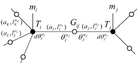
Figure 1: A graphic representation for the GTPS. The open circle which connects to links $I$ and $J$ represents the Grassmann metric $G_{ij,a_{I}a_{J}}$. The solid circle on the physical site $i$ represents the Grassmann tensors $T^{m_{i}}_{i;a_{K}a_{L}...}$. The Grassmann numbers $\theta^{\alpha}_{I}$ associate with the Grasmann metric $G_{ij,a_{I}a_{J}}$ and the dual Grassmann numbers associate with the Grassmann tensor $T^{m_{i}}_{i;a_{K}a_{L}...}$. There are a pair of indices $(a_{I},\{l_{I}^{\alpha_{I}}\})$ live on link $I$. $a_{I}$ is called the bosonic index while $\{l_{I}^{\alpha_{I}}\}=0,1$ are called the fermionic indices.

Let us recall the generic GTPS wavefunctions(defined in the usual Fork basis):

$$\Psi(\{m_{i}\})=\sum_{\{a_{I}\}}P_{0}\int\prod_{i}T^{m_{i}}_{i;a_{K}a_{L}...}\prod_{ij}G_{ij;a_{I}a_{J}},$$ (1)

where

$$T_{i;a_{K}a_{L}...}^{m_{i}}=\sum_{\{l^{\alpha_{K}}_{K}\}\{l^{\alpha_{L}}_{L}\}...}{\rm{T}}^{m_{i};\{l^{\alpha_{K}}_{K}\}\{l^{\alpha_{L}}_{L}\}...}_{i;a_{K}a_{L}...}\prod_{I\in i}\widetilde{\prod_{\alpha_{I}}}(\mathrm{d}\theta^{\alpha_{I}}_{I})^{l^{\alpha_{I}}_{I}}$$

$$G_{ij;a_{I}a_{J}}=\sum_{\{l^{\alpha_{I}}_{I}\}\{l^{\alpha_{J}}_{J}\}}{\rm{G}}^{\{l^{\alpha_{I}}_{I}\}\{l^{\alpha_{J}}_{J}\}}_{ij;a_{I}a_{J}}\prod_{\alpha_{J}}(\theta^{\alpha_{J}}_{J})^{l^{\alpha_{J}}_{J}}\prod_{\alpha_{I}}(\theta^{\alpha_{I}}_{I})^{l^{\alpha_{I}}_{I}}$$ (2)

Here $i,j,\cdots$ label different physical sites, $I,J,\cdots$ label different links and $I\in i$ means the link $I$ connects to the site $i$(See in Fig. 1, any link $I$ uniquely belongs to one physical site $i$). On each link $I$, $a_{I}$ labels the bosonic inner indices, $l_{I}^{\alpha_{I}}=0,1$ labels the fermionic inner indices and $\alpha_{I}$ labels different species of Grassmann variables. $m_{i}$ is the physical index. $\theta^{\alpha_{I}}_{I}$ and $\mathrm{d}\theta^{\alpha_{I}}_{I}$ are Grassmann numbers and dual Grassmann numbers that satisfy the standard Grassmann algebra:

$$\theta^{\alpha_{I}}_{I}\theta^{\alpha^{\prime}_{I^{\prime}}}_{I^{\prime}} =-\theta^{\alpha^{\prime}_{I^{\prime}}}_{I^{\prime}}\theta^{\alpha_{I}}_{I}, \mathrm{d}\theta^{\alpha_{I}}_{I}\mathrm{d}\theta^{\alpha^{\prime}_{I^{\prime}}}_{I^{\prime}} =-\mathrm{d}\theta^{\alpha^{\prime}_{I^{\prime}}}_{I^{\prime}}\mathrm{d}\theta^{\alpha_{I}}_{I},$$

$$\int\mathrm{d}\theta^{\alpha_{I}}_{I}\theta^{\alpha^{\prime}_{I^{\prime}}}_{I^{\prime}} =\delta_{I,I^{\prime}}\delta_{\alpha_{I}\alpha^{\prime}_{I^{\prime}}} \int\mathrm{d}\theta^{\alpha_{I}}_{I}1 =0.$$ (3)

Note that $\prod_{i}$ and $\widetilde{\prod_{i}}$ have opposite orders:

$$\prod_{i}\theta_{i}\equiv\theta_{1}\theta_{2}\theta_{3}...\ \ \ \ \ \ \widetilde{\prod_{i}}\theta_{i}\equiv...\theta_{3}\theta_{2}\theta_{1}.$$ (4)

The symbol $P_{0}$ represents a projection of the result of the integral to the term containing no Grassmann variables $\theta^{\alpha_{I}}_{I}$.

For fermion(electron) systems, the physical index $m_{i}$ in a local Hilbert space is always associated with a definite fermion parity $P_{f}(m_{i})=\pm 1$. Hence, we can impose the following constraints to issue that Eq. (1) does represent fermion wavefunctions.

$$\sum_{I\in i}\sum_{\alpha_{I}}l^{\alpha_{I}}_{I}=\text{odd, if $P_{f}(m_{i})=-1$}$$

$$\sum_{I\in i}\sum_{\alpha_{I}}l^{\alpha_{I}}_{I}=\text{even,if $P_{f}(m_{i})=1$}$$

$$\sum_{\alpha_{I}}l^{\alpha_{I}}_{I}+\sum_{\alpha_{J}}l^{\alpha_{J}}_{J}=\text{even}$$ (5)

Although the original form of Eq.(1) provides us a good physical insight of the state, especially for strongly correlated systems from projective constructions, it is not an efficient representation for numerical simulations. In the following we will derive the standard form of GTPS to simplify the representation.

By using the Grassmann version of the singular-value-decomposition(GSVD) method proposed in Ref.Gu et al. (2010), under the constraint $\sum_{\alpha_{I}}l^{\alpha_{I}}_{I}+\sum_{\alpha_{J}}l^{\alpha_{J}}_{J}=\text{even}$, we can decompose $G_{ij;a_{I}a_{J}}$ into(see Fig. 2):

$$G_{ij;a_{I}a_{J}}=\sum_{p_{I}p_{J}}P_{0}^{\prime}\int g_{ij;q_{I}q_{J}}S_{I;a_{I}q_{I}}S_{J;a_{J}q_{J}}$$ (6)

with

$$g_{ij;q_{I}q_{J}} =(1+\mathrm{d}\theta_{J}\mathrm{d}\theta_{I})\delta_{q_{I}q_{J}}$$

$$S_{I;a_{I}q_{I}} =\sum_{\{l_{I}^{\alpha_{I}}\}n_{I}}{\rm{S}}_{I;a_{I}q_{I}}^{\{l_{I}^{\alpha_{I}}\}n_{I}}\left[\prod_{\alpha_{I}}(\theta^{\alpha_{I}}_{I})^{l^{\alpha_{I}}_{I}}\right]\theta_{I}^{n_{I}}$$

$$S_{J;a_{J}q_{J}} =\sum_{\{l_{J}^{\alpha_{J}}\}n_{J}}{\rm{S}}_{J;a_{J}q_{J}}^{\{l_{J}^{\alpha_{J}}\}n_{J}}\left[\prod_{\alpha_{J}}(\theta^{\alpha_{J}}_{J})^{l^{\alpha_{J}}_{J}}\right]\theta_{J}^{n_{J}}$$ (7)

and

$$n_{I}=n_{J}=\sum_{\alpha_{I}}l^{\alpha_{I}}_{I}\text{ mod }2=\sum_{\alpha_{J}}l^{\alpha_{J}}_{J}\text{ mod }2,$$ (8)

where ${\rm{S}}_{I;a_{I}q_{I}}^{\{l_{I}^{\alpha_{I}}\}n_{I}}=\sqrt{\Lambda_{q_{I},n_{I}}}U_{a_{I}{\{l_{I}^{\alpha_{I}}\}};q_{I},n_{I}}$ and ${\rm{S}}_{J;a_{J}q_{J}}^{\{l_{J}^{\alpha_{J}}\}n_{J}}=\sqrt{\Lambda_{q_{J},n_{J}}}V_{a_{J}{\{l_{J}^{\alpha_{J}}\}};q_{J},n_{J}}$ are determined by the singular-value-decomposition(SVD) for the matrix $M_{a_{I}{\{l_{I}^{\alpha_{I}}\};a_{J}{\{l_{J}^{\alpha_{J}}\}}}}={\rm{G}}^{\{l^{\alpha_{I}}_{I}\}\{l^{\alpha_{J}}_{J}\}}_{ij;a_{I}a_{J}}$ with $M=U\Lambda V^{T}$. (Notice that the constraint $\sum_{\alpha_{I}}l^{\alpha_{I}}_{I}+\sum_{\alpha_{J}}l^{\alpha_{J}}_{J}=\text{even}$ implies a $Z_{2}$ symmetry for the matrix $M$ which can be block diagonalized, with each sector labeled as $n_{I}=n_{J}=0$ or $1$.) Again, the symbol $P_{0}^{\prime}$ represents a projection of the result of the integral to the term containing no Grassmann number $\theta_{I}$. We call $g_{ij;q_{I}q_{J}}$ the standard metric for GTPS, which is the Grassmann generalization of the canonical delta function $\delta_{q_{I}q_{J}}$.

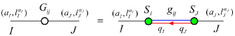
Figure 2: A graphic representation of the decomposition Eq. (6). We use double lines(red and blue) to represent the standard metric $g_{ij}$, which is the $Z_{2}$ graded version of the canonical delta function. The blue line represents the channel with no inner fermion($n_{I}=n_{J}=0$) and the red line represents the channel with one inner fermion($n_{I}=n_{J}=1$) for the standard metric. The arrow of the red line represents the ordering for the dual Grassmann variables $\mathrm{d}\theta_{I}$ and $\mathrm{d}\theta_{J}$. We notice that the standard metric $g_{ij}$ only has one species of Grassmann variable despite the original Grassmann metric $G_{ij}$ contains many species of Grassmann variables on its link $I$ and $J$(labeled by $\alpha_{I}$ and $\alpha_{J}$). Here $q_{I},q_{J}$ and $a_{I},a_{J}$ are bosonic indices.

Put Eq.(6) into Eq.(1), we have:

$$\Psi(\{m_{i}\}) =\sum_{\{a_{I}\},\{q_{I}\}}P_{0}P_{0}^{\prime}\int\prod_{ij}g_{ij;q_{I}q_{J}}$$

$$\times\prod_{i}T^{m_{i}}_{i;a_{K}a_{L}...}\prod_{I}S_{I;a_{I}q_{I}},$$ (9)

The Grassmann matrices $S_{I;a_{I}q_{I}}$ defined on all links contain even number of Grassmann numbers and they commute with each other. Such a property allows us to regroup them as:

$$\prod_{I}S_{I;a_{I}q_{I}}=\widetilde{\prod_{i}}\widetilde{\prod_{I\in i}}S_{I;a_{I}q_{I}},$$ (10)

To derive the above expression, we use the fact that each link $I$ uniquely belongs to a site $i$. $\widetilde{\prod}$ defined here has opposite orders according to that defined in Eq. (2)

Thus, we can integral out all the Grassmann numbers $\prod_{\alpha_{I}}(\theta^{\alpha_{I}}_{I})^{l^{\alpha_{I}}_{I}}$ and sum over all the bosonic indices $\{a_{I}\}$ to derive a simplified wave function:

$$\Psi(\{m_{i}\})=\sum_{\{q_{I}\}}P_{0}^{\prime}\int\prod_{ij}g_{ij;q_{I}q_{J}}\prod_{i}\widetilde{T}^{m_{i}}_{i;q_{K}q_{L}...},$$ (11)

where the new Grassmann tensor $\widetilde{T}_{i;a_{K}a_{L}...}^{m_{i}}$ associated with physical site $i$ can be expressed as(see Fig. 3):

$$\widetilde{T}_{i;q_{K}q_{L}...}^{m_{i}}=\sum_{n_{K}n_{L}...}\widetilde{\rm{T}}^{m_{i};n_{K}n_{L}...}_{i;q_{K}q_{L}...}\prod_{I\in i}\theta_{I}^{n_{I}}$$ (12)

with

$$\widetilde{\rm{T}}^{m_{i};n_{K}n_{L}...}_{i;q_{K}q_{L}...} =\sum_{a_{K}a_{L}...}\sum_{\{l^{\alpha_{K}}_{K}\}\{l^{\alpha_{L}}_{L}\}...}$$

$${\rm{T}}^{m_{i};\{l^{\alpha_{K}}_{K}\}\{l^{\alpha_{L}}_{L}\}...}_{i;a_{K}a_{L}...}\prod_{I\in i}{\rm{S}}_{I;a_{I}q_{I}}^{\{l_{I}^{\alpha_{I}}\}n_{I}}$$ (13)

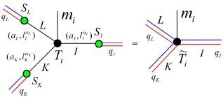
Figure 3: A graphic representation for the standard Grassmann tensor $\widetilde{T}_{i}$, which is a combination of the Grassmann tensor $T_{i}$ and those $S_{I(K,L)}$(green solid circles) surrounding it.

We call Eq.(11) the standard form(see Fig. 4) of GTPS which only contains one species of Grassmann variable on each link. We can further simplify the expression by grouping the bosonic index $q_{I}$ and fermionic index $n_{I}$ into one super index $p_{I}=(q_{I},n_{I})$.

$$\Psi(\{m_{i}\})=\sum_{\{p_{I}\}}\int\prod_{ij}\mathbf{g}_{ij;p_{I}p_{J}}\prod_{i}\mathbf{T}^{m_{i}}_{i;p_{K}p_{L}...},$$ (14)

with

$$\mathbf{g}_{ij;p_{I}p_{J}} =\delta_{p_{I}p_{J}}(\mathrm{d}\theta_{J})^{N_{f}(p_{J})}(\mathrm{d}\theta_{I})^{N_{f}(p_{I})}$$

$$\mathbf{T}^{m_{i}}_{i;p_{K}p_{L}...} =\widetilde{\rm{T}}^{m_{i};n_{K}n_{L}...}_{i;q_{K}q_{L}...}\prod_{I\in i}(\theta_{I})^{N_{f}(p_{I})},$$ (15)

where $N_{f}(p_{I})=n_{I}$. Notice that the super index $p_{I}$ has a definite fermion parity $P_{f}(p_{I})=\pm 1$ and the corresponding fermion number is determined as $N_{f}=\frac{P_{f}+1}{2}$.

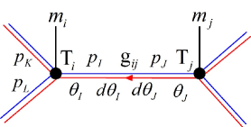
Figure 4: A graphic representation for the standard form of GTPS. The solid circle on the physical site $i$ represents the standard Grassmann tensors $\mathbf{T}^{m_{i}}_{i;p_{K}p_{L}...}$. The link index $p_{I}$ has a definite fermion parity $P_{f}$ and we use the blue(red) line to represent the fermion parity even(odd) $P_{f}(p_{I})=1(-1)$ indices. If $P_{f}(p_{I})=-1$, we associate a Grassmann number $\theta_{I}$ with the standard Grassmann tensor $\mathbf{T}^{m_{i}}_{i;p_{K}p_{L}...}$ while associate its dual $\mathrm{d}\theta_{I}$ with the standard metric $\mathbf{g}_{ij,p_{I}p_{J}}$. Since the standard metric $\mathbf{g}_{ij,p_{I}p_{J}}$ is actually just a Grassmann generalization of the canonical delta function $\delta_{p_{I}p_{J}}$, we only need to use an arrow to specify the ordering of the two Grassmann variables $\mathrm{d}\theta_{J}$ and $\mathrm{d}\theta_{I}$.

The new form Eq.(14) is extremely useful in general purpose of numerical calculations. We will use this new form to explain all the details of our algorithms.

III The imaginary time evolution algorithm

In this section, we will start with a brief review of imaginary time evolution algorithms for TPS and then generalize all those algorithms into GTPS. Finally, we apply the algorithms to some fermion models on honeycomb lattice.

III.1 A review of the algorithm of TPS

III.1.1 generic discussion

Let us consider the imaginary time evolution for generic TPS $|\Psi_{0}\rangle$.

$$|\Psi_{\tau}\rangle=e^{-\tau H}|\Psi_{0}\rangle$$ (16)

If we don’t make any approximation, the true ground state can be achieved in the $\tau\rightarrow\infty$ limit.

$$|\Psi_{GS}\rangle=\lim_{\tau\rightarrow\infty}e^{-\tau H}|\Psi_{0}\rangle=\lim_{N\rightarrow\infty}e^{-N\delta\tau H}|\Psi_{0}\rangle,$$ (17)

where $N$ is the number of evolution steps and $\delta\tau=\tau/N$ is a sufficiently thin imaginary-time slice. However, without any approximation, the inner dimension of TPS will increase exponentially as the number of evolution steps increase. Hence, we need to find out the best TPS approximation with fixed inner dimension.

Without loss of generality(WLOG), we use the honeycomb lattice geometry to explain the details here and for the rest of the paper. To illustrate the key idea of the algorithm, let us consider a simple case that the model Hamiltonian $H$ only contains a summation of nearest neighbor two-body terms:

$$H=\sum_{\langle ij\rangle}h_{ij}.$$ (18)

Let us divide the Hamiltonian into three parts:

$$H=H_{x}+H_{y}+H_{z};\quad H_{\alpha}=\sum_{i\in A}h_{i,i+\alpha}\quad(\alpha=x,y,z),$$ (19)

where $A$ labels the sublattices $A$ and $x,y,z$ label three different nearest-neighbor directions. By applying the Trotter expansion, we have:

$$e^{-\delta\tau H}=e^{-\delta\tau H_{x}}e^{-\delta\tau H_{y}}e^{-\delta\tau H_{z}}+o(\delta\tau^{2})$$ (20)

Notice that each $H_{\alpha}$ only contains summation of commuting terms, hence we can decompose them without error:

$$e^{-\delta\tau H_{\alpha}}=\prod_{i}e^{-\delta\tau h_{i,i+\alpha}}$$ (21)

Let us expand $|\Psi_{0}\rangle$ under the physical basis:

$$|\Psi_{0}\rangle =\sum_{\{m_{i},m_{j}\}}\sum_{\{a,a^{\prime}\}}\prod_{i\in A}{T}_{i;abc}^{m_{i}}\prod_{j\in B}{T}_{j;a^{\prime}b^{\prime}c^{\prime}}^{m_{j}}$$

$$\prod_{ij}\delta_{aa^{\prime}}|\{m_{i},m_{j}\}\rangle,$$ (22)

Here $A,B$ denote two different sublattices in a unit cell and $m_{i(j)}$ denote the physical indices on site $i(j)$, e.g., $m_{i(j)}=\uparrow,\downarrow$ for a spin $1/2$ system. The canonical delta function $\delta_{aa^{\prime}}$ defined on link $ij$ can be regarded as the metric associated with tensor contraction, which can be generalized to its Grassmann variable version for fermion systems. After acting one evolution operator $e^{-\delta\tau h_{ij}}$ onto the corresponding link $ij$, we can expand the new state $e^{-\delta\tau h_{ij}}|\Psi_{0}\rangle$ as:

$$e^{-\delta\tau h_{ij}}|\Psi_{0}\rangle =\sum_{\{m_{i},m_{j}\}}\sum_{\{a,a^{\prime}\}}\sum_{m_{i}^{\prime}m_{j}^{\prime}}E_{m_{i}^{\prime}m_{j}^{\prime}}^{m_{i}m_{j}}T_{i;abc}^{m_{i}^{\prime}}T_{j;a^{\prime}b^{\prime}c^{\prime}}^{m_{j}^{\prime}}$$

$$\times\prod_{i^{\prime}\neq i}T_{i^{\prime};edf}^{m_{i^{\prime}}}\prod_{j^{\prime}\neq j}T_{j^{\prime};e^{\prime}d^{\prime}f^{\prime}}^{m_{j^{\prime}}}\prod_{ij}\delta_{aa^{\prime}}|\{m_{i},m_{j}\}\rangle$$ (23)

where $E_{m_{i}^{\prime}m_{j}^{\prime}}^{m_{i}m_{j}}=\langle m_{i}m_{j}|e^{-\delta\tau h_{ij}}|m_{i}^{\prime}m_{j}^{\prime}\rangle$ is the matrix element of the evolution operator on link $ij$. Using the SVD decomposition, we can decompose the rank $6$ tensor $T_{ij;m_{i}m_{j}bcb^{\prime}c^{\prime}}=\sum_{a}\sum_{m_{i}^{\prime}m_{j}^{\prime}}E_{m_{i}^{\prime}m_{j}^{\prime}}^{m_{i}m_{j}}T_{i;abc}^{m_{i}^{\prime}}T_{j;ab^{\prime}c^{\prime}}^{m_{j}^{\prime}}$ as:

$$T_{ij;m_{i}m_{j}bcb^{\prime}c^{\prime}}=\sum_{aa^{\prime}}{\mathcal{T}}^{m_{i}}_{i;abc}{\mathcal{T}}^{m_{j}}_{j;a^{\prime}b^{\prime}c^{\prime}}\delta_{aa^{\prime}}.$$ (24)

Here the indices $a,a^{\prime}$ have dimension $Dd^{2}$, where $D$ is the inner dimension and $d$ is the physical dimension of the tensor $T_{i;abc}^{m_{i}}$. After applying $e^{-\delta\tau H_{x}}$ on state $|\Psi_{0}\rangle$, the tensor $T_{i}$ will be replaced by $\mathcal{T}_{i}$:

$$e^{-\delta\tau H_{x}}|\Psi_{0}\rangle =\sum_{\{m_{i},m_{j}\}}\sum_{\{a,a^{\prime}\}}\prod_{i\in A}{\mathcal{T}}_{i;abc}^{m_{i}}\prod_{j\in B}{\mathcal{T}}_{j;a^{\prime}b^{\prime}c^{\prime}}^{m_{j}}$$

$$\times\prod_{ij}\delta_{aa^{\prime}}|\{m_{i},m_{j}\}\rangle,$$ (25)

Notice that all $\{{\mathcal{T}}_{i;abc}^{m_{i}}\}$ have enlarged inner dimension $Dd^{2}$ instead of $D$ for their inner indices $a$(the bond along $x$ direction). Similarly, the dimension of indices $b,c$(the bonds along $y,z$ directions) will also be enlarged to $Dd^{2}$ after applying $e^{-\delta\tau H_{y}}$ and $e^{-\delta\tau H_{z}}$ on $|\Psi_{0}\rangle$. Thus, it is easy to see that the inner dimension will increase exponentially as evolution steps increase if we don’t make any truncation.

To solve the above difficulty, we need to find a new set of $\{{T^{\prime}}_{i;abc}^{m_{i}}\}$ with fixed inner dimension $D$ that minimizes the distance with $e^{-\delta\tau H_{x}}|\Psi_{0}\rangle$. If we start from $|\Psi_{0}\rangle$ and evolve it by $e^{-\delta\tau H_{x}}$ in a sufficiently thin time slice, the cost function $f$ takes the form:

$$f(\{{T^{\prime}}_{i;abc}^{m_{i}}\})=|||\Psi_{0}^{\prime}\rangle-e^{-\delta\tau H_{x}}|\Psi_{0}\rangle||$$

$$=\langle\Psi_{0}^{\prime}|\Psi_{0}^{\prime}\rangle-\left(\langle\Psi_{0}^{\prime}|e^{-\delta\tau H_{x}}|\Psi_{0}\rangle+h.c.\right)+const.,$$ (26)

where

$$|\Psi_{0}^{\prime}\rangle =\sum_{\{m_{i},m_{j}\}}\sum_{\{a,a^{\prime}\}}\prod_{i\in A}{T^{\prime}}_{i;abc}^{m_{i}}\prod_{j\in B}{T^{\prime}}_{j;a^{\prime}b^{\prime}c^{\prime}}^{m_{j}}$$

$$\prod_{ij}\delta_{aa^{\prime}}|\{m_{i},m_{j}\}\rangle,$$ (27)

$f$ is a multi-variable quadratic function of $\{{T^{\prime}}_{i;x_{i}y_{i}z_{i}}^{m_{i}}\}$, hence we can use the sweep method to minimize it. The advantage of the above algorithm is that the Trotter error will not accumulate after long time evolution. However, calculating the cost function $f$ explicitly is an exponentially hard problem and we need further approximations at this stage. Some possible methods have been proposed based on the MPS algorithmMurg et al. (2007), but the calculational cost can still be very big and the method has only been implemented with the open boundary condition(OBC) so far.

III.1.2 Translational invariant systems

Nevertheless, for translational invariant TPS ansatz, it is possible to develop an efficient method to simulate the cost function by using the TERG method.

We assume that $T_{i}=T_{A}$ if $i\in A$ and $T_{j}=T_{B}$ if $j\in B$. The cost function can be expressed as:

$$f(T^{\prime}_{A},T^{\prime}_{B}) =\rho^{bcb^{\prime}c^{\prime};\bar{b}\bar{c}\bar{b}^{\prime}\bar{c}^{\prime}}{\bar{T^{\prime}}}_{A;\bar{a}\bar{b}\bar{c}}^{m_{i}}{T^{\prime}}_{A;abc}^{m_{i}}{\bar{T^{\prime}}}_{B;\bar{a}\bar{b}^{\prime}\bar{c}^{\prime}}^{m_{j}}{T^{\prime}}_{B;ab^{\prime}c^{\prime}}^{m_{j}}$$

$$-\left(e^{\bar{b}\bar{c}\bar{b}^{\prime}\bar{c}^{\prime};m_{i}m_{j}}{\bar{T^{\prime}}}_{A;\bar{a}\bar{b}\bar{c}}^{m_{i}}{\bar{T^{\prime}}}_{B;\bar{a}\bar{b}^{\prime}\bar{c}^{\prime}}^{m_{j}}+h.c.\right)$$

$$+const,$$ (28)

where $\rho$ and $e$(Fig. 5) are the so called environment tensors. Here we use the convention that all the repeated indices will be summed over and we use $\bar{T}$ to represent complex conjugate of $T$. Strictly speaking, the environment tensors for $\rho$ and $e$ are also dependent on $T_{A}^{\prime}$ and $T_{B}^{\prime}$, thus $f$ is no longer a quadratic multi-variable function. However, for sufficiently thin time slice, up to $o(\delta\tau^{2})$ error(same order as Trotter error), we can replace $T_{A}^{\prime},T_{B}^{\prime}$ by $T_{A},T_{B}$ when calculating the environment tensor $\rho$. $e$ can be derived from $\rho$:

$$e^{\bar{b}\bar{c}\bar{b}^{\prime}\bar{c}^{\prime};m_{i}m_{j}}=\rho^{bcb^{\prime}c^{\prime};\bar{b}\bar{c}\bar{b}^{\prime}\bar{c}^{\prime}}E_{m_{i}^{\prime}m_{j}^{\prime}}^{m_{i}m_{j}}{T}_{A;abc}^{m_{i}^{\prime}}{T}_{B;ab^{\prime}c^{\prime}}^{m_{j}^{\prime}}$$ (29)

Again, repeated indices need to be summed over here. We notice that $\rho$ can be expressed as a tensor trace of double tensors $\mathbb{T}_{A(B)}=\sum_{m}\bar{T}_{A(B)}^{m}\otimes T_{A(B)}^{m}$ with an impurity tensor $\mathbb{T}_{ij}$ for the link $ij$(see Fig. 6):

$$\rho^{bcb^{\prime}c^{\prime};\bar{b}\bar{c}\bar{b}^{\prime}\bar{c}^{\prime}}={\rm{tTr}}[\mathbb{T}_{ij}^{\rho}\otimes\mathbb{T}_{A}\otimes\mathbb{T}_{B}\otimes\mathbb{T}_{A}\otimes\mathbb{T}_{B}\cdots],$$ (30)

where the impurity double tensor $\mathbb{T}_{ij}$ is just a projector:

$$\mathbb{T}_{ij;bcb^{\prime}c^{\prime};\bar{b}\bar{c}\bar{b}^{\prime}\bar{c}^{\prime}}=1;\quad{\rm{others}}=0$$ (31)

Now it is easy to see that we can first decompose the impurity tensor on the link $i,j$ to two rank $3$ impurity tensors on site $i,j$ and then implement the usual TERG algorithm. We can also use a more efficient but complicated way to compute $\rho$ by applying the coarse graining procedures for all sites except sites $i,j$, as introduced in Ref.Z.Y. et al. (2008-2010).

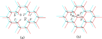
Figure 5: A graphic representation for the environment tensor $\rho$((a)) and $e$((b)) on honeycomb lattice.

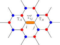
Figure 6: A graphic representation for the tensor contraction that allow us to compute $\rho$ on honeycomb lattice.

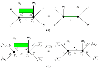
Figure 7: (a)After applying the two body evolution operator $e^{-\delta\tau h_{ij}}$ to the $ij$ link for TPS(with inner dimension $D$), we get new TPS with enlarged inner dimension($Dd^{2}$, $d$ is the physical dimension) for the corresponding link. (b) For large classes of translational invariant TPS, we can reduce the inner dimension from $Dd^{2}$ back to $D$ with respect to some environment wight $\Lambda$.

The above algorithm can further be simplified if we assume that the environment tensor $\rho$ has specific forms for certain physical systems. One interesting attempt was proposed in Ref.Jiang et al. (2008) by assuming that $\rho$ can be factorized as:

$$\rho^{bcb^{\prime}c^{\prime};\bar{b}\bar{c}\bar{b}^{\prime}\bar{c}^{\prime}}=\Lambda_{b}^{y}\Lambda_{c}^{z}\Lambda_{b^{\prime}}^{y}\Lambda_{c^{\prime}}^{z}\delta_{b\bar{b}}\delta_{c\bar{c}}\delta_{b^{\prime}\bar{b}^{\prime}}\delta_{c^{\prime}\bar{c}^{\prime}},$$ (32)

where $\Lambda^{\alpha}$ is a positive weight vector defined on links along $\alpha$ direction. The above form can always be true for 1D systemsVidal et al. (2007) due to the existence of the canonical form of an MPS. Although the above form is not generic enough in 2D, it still works well in many cases, especially for those systems with symmetry breaking order. In this case, the cost function Eq.(28) can be solved by SVD decomposition and keep the leading $D$th singular values for the following matrix(see Fig. 43):

$$M_{bcm_{i};b^{\prime}c^{\prime}m_{j}} =\sum_{a,m_{i}^{\prime},m_{j}^{\prime}}\sqrt{\Lambda_{b}^{y}}\sqrt{\Lambda_{c}^{z}}\sqrt{\Lambda_{b^{\prime}}^{y}}\sqrt{\Lambda_{c^{\prime}}^{z}}T_{ij,m_{i}n_{j}bcb^{\prime}c^{\prime}}$$

$$=\sum_{a,m_{i}^{\prime},m_{j}^{\prime}}\sqrt{\Lambda_{b}^{y}}\sqrt{\Lambda_{c}^{z}}\sqrt{\Lambda_{b^{\prime}}^{y}}\sqrt{\Lambda_{c^{\prime}}^{z}}$$

$$\times E_{m_{i}^{\prime}m_{j}^{\prime}}^{m_{i}m_{j}}{T}_{A;abc}^{m_{i}^{\prime}}{T}_{B;ab^{\prime}c^{\prime}}^{m_{j}^{\prime}}$$

$$\simeq\sum_{a=1}^{D}U_{bcm_{i};a}V_{b^{\prime}c^{\prime}m_{j};a}\Lambda_{a}^{\prime}$$ (33)

The new tensors $T^{\prime}_{A}$ and $T^{\prime}_{B}$ can be determined as:

$${T^{\prime}}^{m_{i}}_{A;abc} =\frac{\sqrt{\Lambda_{a}^{\prime}}}{\sqrt{\Lambda_{b}^{y}}\sqrt{\Lambda_{c}^{z}}}U_{bcm_{i};a}$$

$${T^{\prime}}^{m_{j}}_{B;a^{\prime}b^{\prime}c^{\prime}} =\frac{\sqrt{\Lambda_{a^{\prime}}^{\prime}}}{\sqrt{\Lambda_{b^{\prime}}^{y}}\sqrt{\Lambda_{c^{\prime}}^{z}}}V_{b^{\prime}c^{\prime}m_{j};a^{\prime}}$$ (34)

Similarly as in 1D, the environment weight associated with bonds along $x$ direction is updated as $\Lambda^{x}=\Lambda^{\prime}$. It is not hard to understand why the above simplified algorithm works very well for systems with symmetry breaking orders, but not in the critical region, since in those cases the ground states are close to product states and the entanglements between the $x,y,z$ directions in the environment tensors become pretty weak. However, for topologically ordered states, the environment tensors can be more complicated. For example, the $Z_{2}$ topologically ordered state in the toric code model will have an emergent $Z_{2}$ symmetry and can not be factorized as a product. Hence, for topological ordered states, it is important to calculate the full environment in the imaginary time evolution.

III.2 Generalize to fermion(electron) systems

In this subsection, we will show how to generalize the above algorithms to GTPS. The key step is to introduce fermion coherent state representation and treat the physical indices also as a Grassmann variable. WLOG, we use a spinless fermion system as a simple example here and for the rest part of the paper:

$$|\eta\rangle\equiv\prod_{i}(1-\eta_{i}c_{i}^{\dagger})|0\rangle,$$ (35)

where $\eta_{i}$ is a Grassmann number.

As already discussed in Ref.Gu et al. (2010), under this new basis, the GTPS wavefunction Eq.(1) and its standard form Eq.(14) can be represented as:

$$\Psi(\{\eta_{i}\})= \sum_{\{m_{i}\}}\sum_{\{a_{I}\}}\int\prod_{i}{\bar{\eta}_{i}}^{m_{i}}T^{m_{i}}_{i;a_{K}a_{L}...}\prod_{ij}G_{ij;a_{I}a_{J}}$$

$$= \sum_{\{m_{i}\}}\sum_{\{p_{I}\}}\int\prod_{ij}\mathbf{g}_{ij;p_{I}p_{J}}\prod_{i}{\bar{\eta}_{i}}^{m_{i}}\mathbf{T}^{m_{i}}_{i;p_{K}p_{L}...}$$

$$= \sum_{\{m_{i}\}}\sum_{\{p_{I}\}}\int\prod_{ij}\mathbf{g}_{ij;p_{I}p_{J}}\prod_{i}\mathbf{\widetilde{T}}^{m_{i}}_{i;p_{K}p_{L}...}$$ (36)

where $\bar{\eta}_{i}$ is the complex conjugate of the Grassmann number $\eta_{i}$ and $\mathbf{\widetilde{T}}^{m_{i}}_{i;p_{K}p_{L}...}={\bar{\eta}_{i}}^{m_{i}}\mathbf{T}^{m_{i}}_{i;p_{K}p_{L}...}$.

On honeycomb lattice with translational invariance, we can simplify the above expression as:

$$\Psi(\{\bar{\eta}_{i}\},\{\bar{\eta}_{j}\})$$ (37)

$$=\sum_{\{m_{i}\},\{m_{j}\}}\sum_{\{a\},\{a^{\prime}\}}\int\prod_{\langle ij\rangle}\textbf{g}_{aa^{\prime}}\prod_{i\in A}{\mathbf{\widetilde{T}}}^{m_{i}}_{A;abc}\prod_{j\in B}{\mathbf{\widetilde{T}}}^{m_{j}}_{B;a^{\prime}b^{\prime}c^{\prime}},$$

with

$${\mathbf{\widetilde{T}}}^{m_{i}}_{A;abc} = {\rm{\widetilde{T}}}^{m_{i}}_{A;abc}\bar{\eta}_{i}^{m_{i}}\theta_{\alpha}^{N_{f}(a)}\theta_{\beta}^{N_{f}(b)}\theta_{\gamma}^{N_{f}(c)},$$

$${\mathbf{\widetilde{T}}}^{m_{j}}_{B;a^{\prime}b^{\prime}c^{\prime}} = {\rm{\widetilde{T}}}^{m_{j}}_{B;a^{\prime}b^{\prime}c^{\prime}}\bar{\eta}_{j}^{m_{j}}\theta_{\alpha^{\prime}}^{N_{f}(a^{\prime})}\theta_{\beta^{\prime}}^{N_{f}(b^{\prime})}\theta_{\gamma^{\prime}}^{H_{f}(c^{\prime})},$$

$$\textbf{g}_{aa^{\prime}} = \delta_{aa^{\prime}}{\mathrm{d}\theta}_{\alpha}^{N_{f}(a)}{\mathrm{d}\theta}_{\alpha^{\prime}}^{N_{f}(a^{\prime})}.$$ (38)

Comparing to usual TPS, here the link indices $\{a,a^{\prime}\}$ always have definite fermion parity $P_{f}=\pm 1$. $N_{f}=0$ when $P_{f}=1$ while $N_{f}=1$ when $P_{f}=-1$.

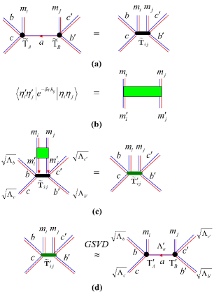
Figure 8: A graphic representation for the simplified imaginary time evolution algorithm for Grassmann tensor product states. In step (a), we sum over the inner indices and integral out the Grassmann variables on the shared link for two adjoint Grassmann tensors $\mathbf{\widetilde{T}}_{A}$ and $\mathbf{\widetilde{T}}_{B}$. In step (b), we express the two sites evolution operator $e^{-\delta\tau h_{ij}}$ under the fermion coherent basis. In step (c) and (d), we apply the evolution operator $e^{-\delta\tau h_{ij}}$ to the two sites Grassmann tensor $\mathbf{\widetilde{T}}_{ij}$ and derive a new two sites Grassmann tensor $\mathbf{\widetilde{T}}_{ij}^{\prime}$. Then we approximate it by two new adjoint Grassmann tensors $\mathbf{\widetilde{T}}_{A}^{\prime}$ and $\mathbf{\widetilde{T}}_{B}^{\prime}$ with respect to the environment weights $\Lambda$. We also use double lines to label different fermion parities for the physical indices. For the simple spinless fermion example, the red line represents one fermion state and the blue line represents the empty state. The metric $(1+\eta_{i}\bar{\eta}_{i})$ is the standard metric for the physical indices.

Let us start from the simplest case with the assumption that the environment can also be approximately represented by some weights. In this case, the imaginary time evolution for GTPS can be reduced to an SVD problem of Grassmann variables. The Grassmann version of the matrix $M$ in Eq.(33) can be constructed as followings(see Fig. 8):

(a) Let us first sum over the bond indices $a,a^{\prime}$ and integrate out the Grassmann variables $\theta_{\alpha},\theta_{\alpha^{\prime}}$:

$$\mathbf{\widetilde{T}}_{ij;m_{i}m_{j}bcb^{\prime}c^{\prime}} =\sum_{aa^{\prime}}\int\mathbf{g}_{aa^{\prime}}\mathbf{\widetilde{T}}_{abc}^{m_{i}}\mathbf{\widetilde{T}}_{a^{\prime}b^{\prime}c^{\prime}}^{m_{j}}$$

$$=\sum_{a}\int{\mathrm{d}\theta}_{\alpha}^{N_{f}(a)}{\mathrm{d}\theta}_{\alpha^{\prime}}^{N_{f}(a)}{\rm{\widetilde{T}}}^{m_{i}}_{A;abc}\bar{\eta}_{i}^{m_{i}}\theta_{\alpha}^{N_{f}(a)}\theta_{\beta}^{N_{f}(b)}\theta_{\gamma}^{N_{f}(c)}{\rm{\widetilde{T}}}^{m_{j}}_{B;ab^{\prime}c^{\prime}}\bar{\eta}_{j}^{m_{j}}\theta_{\alpha^{\prime}}^{N_{f}(a)}\theta_{\beta^{\prime}}^{N_{f}(b^{\prime})}\theta_{\gamma^{\prime}}^{H_{f}(c^{\prime})}$$

$$=\sum_{a}(-)^{\left[m_{i}+m_{j}\right]N_{f}(a)}(-)^{m_{j}\left[m_{i}+N_{f}(b)+N_{f}(c)\right]}{\rm{\widetilde{T}}}^{m_{i}}_{A;abc}{\rm{\widetilde{T}}}^{m_{j}}_{B;ab^{\prime}c^{\prime}}\bar{\eta}_{j}^{m_{j}}\bar{\eta}_{i}^{m_{i}}\theta_{\beta}^{N_{f}(b)}\theta_{\gamma}^{N_{f}(c)}\theta_{\beta^{\prime}}^{N_{f}(b^{\prime})}\theta_{\gamma^{\prime}}^{N_{f}(c^{\prime})}.$$ (39)

Here the sign factor $(-)^{\left[m_{i}+m_{j}\right]N_{f}(a)}(-)^{m_{j}\left[m_{i}+N_{f}(b)+N_{f}(c)\right]}$ comes from the anti-commutating relations of Grassmann variables.

(b) Next we derive the matrix element of the evolution operator under fermion coherent state representation. Let us first calculate them under the usual Fock basis $(c_{j}^{\dagger})^{m_{j}}(c_{i}^{\dagger})^{m_{i}}|0\rangle$ with $m_{i},m_{j}=0,1$. Let us define:

$$E_{m_{i}^{\prime}m_{j}^{\prime}}^{m_{i}m_{j}}=\langle 0|(c_{i})^{m_{i}}(c_{j})^{m_{j}}e^{-\delta\tau h_{ij}}(c_{j}^{\dagger})^{m_{j}^{\prime}}(c_{i}^{\dagger})^{m_{i}^{\prime}}|0\rangle$$ (40)

Thus, we can expand $e^{-\delta\tau h_{ij}}$ as:

$$e^{-\delta\tau h_{ij}}=\sum_{m_{i}m_{j};m_{i}^{\prime}m_{j}^{\prime}}E_{m_{i}^{\prime}m_{j}^{\prime}}^{m_{i}m_{j}}(c_{j}^{\dagger})^{m_{j}}(c_{i}^{\dagger})^{m_{i}}|0\rangle\langle 0|(c_{i})^{m_{i}^{\prime}}(c_{j})^{m_{j}^{\prime}}$$ (41)

In the fermion coherent state basis, we have:

$$\langle\eta^{\prime}_{i},\eta^{\prime}_{j}|e^{-\delta\tau h_{ij}}|\eta_{i},\eta_{j}\rangle$$

$$= \sum_{m_{i}m_{j};m_{i}^{\prime}m_{j}^{\prime}}E_{m_{i}^{\prime}m_{j}^{\prime}}^{m_{i}m_{j}}(\bar{\eta}^{\prime}_{j})^{m_{j}}(\bar{\eta}^{\prime}_{i})^{m_{i}}(\eta_{i})^{m_{i}^{\prime}}(\eta_{j})^{m_{j}^{\prime}}$$ (42)

(c) Then we can evolve the state $\Psi$ to a new state $\Psi^{\prime}$:

$$\Psi^{\prime}(\{\bar{\eta}_{i}^{\prime}\},\{\bar{\eta}_{j}^{\prime}\}) =\int\mathrm{d}\bar{\eta}_{i}\mathrm{d}\eta_{i}\mathrm{d}\bar{\eta}_{j}\mathrm{d}\eta_{j}(1+\eta_{i}\bar{\eta}_{i})(1+\eta_{j}\bar{\eta}_{j})$$

$$\times\langle\eta^{\prime}_{i},\eta^{\prime}_{j}|e^{-\delta\tau h_{ij}}|\eta_{i},\eta_{j}\rangle\Psi(\{\bar{\eta}_{i}\},\{\bar{\eta}_{j}\}).$$ (43)

Put Eq.(39) and Eq.(42) into the above equation, it is easy to derive the Grassmann version of the rank $6$ tensor $T_{ij}$ defined on the link $ij$. We have:

$$\mathbf{\widetilde{T}}_{ij;m_{i}m_{j}bcb^{\prime}c^{\prime}}^{\prime} =\sum_{m_{i}^{\prime}m_{j}^{\prime}a}(-)^{\left[m_{i}^{\prime}+m_{j}^{\prime}\right]N_{f}(a)}(-)^{m_{j}^{\prime}\left[m_{i}^{\prime}+N_{f}(b)+N_{f}(c)\right]}E_{m_{i}^{\prime}m_{j}^{\prime}}^{m_{i}m_{j}}{\rm{\widetilde{T}}}^{m_{i}^{\prime}}_{A;abc}{\rm{\widetilde{T}}}^{m_{j}^{\prime}}_{B;ab^{\prime}c^{\prime}}{(\bar{\eta}_{j}^{\prime})}^{m_{j}}{(\bar{\eta}_{i}^{\prime})}^{m_{i}}\theta_{\beta}^{N_{f}(b)}\theta_{\gamma}^{N_{f}(c)}\theta_{\beta^{\prime}}^{N_{f}(b^{\prime})}\theta_{\gamma^{\prime}}^{N_{f}(c^{\prime})}$$

$$=\sum_{m_{i}^{\prime}m_{j}^{\prime}a}(-)^{\left[m_{i}^{\prime}+m_{j}^{\prime}\right]N_{f}(a)}(-)^{m_{j}^{\prime}\left[m_{i}^{\prime}+N_{f}(b)+N_{f}(c)\right]}(-)^{m_{j}\left[m_{i}+N_{f}(b)+N_{f}(c)\right]}$$

$$\times E_{m_{i}^{\prime}m_{j}^{\prime}}^{m_{i}m_{j}}{\rm{\widetilde{T}}}^{m_{i}^{\prime}}_{A;abc}{\rm{\widetilde{T}}}^{m_{j}^{\prime}}_{B;ab^{\prime}c^{\prime}}{(\bar{\eta}_{i}^{\prime})}^{m_{i}}\theta_{\beta}^{N_{f}(b)}\theta_{\gamma}^{N_{f}(c)}{(\bar{\eta}_{j}^{\prime})}^{m_{j}}\theta_{\beta^{\prime}}^{N_{f}(b^{\prime})}\theta_{\gamma^{\prime}}^{N_{f}(c^{\prime})}.$$ (44)

We notice that there will be an extra sign factor $(-)^{m_{j}\left[m_{i}+N_{f}(b)+N_{f}(c)\right]}$ after we reorder these Grassmann variables.

(d) Finally, we can define the Grassmann generalization of the $M$ matrix after putting the environment weight for all the inner indices.

$$\mathbf{M}_{bcm_{i};b^{\prime}c^{\prime}m_{j}} ={\rm{M}}_{bcm_{i};b^{\prime}c^{\prime}m_{j}}{(\bar{\eta}_{i}^{\prime})}^{m_{i}}\theta_{\beta}^{N_{f}(b)}\theta_{\gamma}^{N_{f}(c)}$$

$$\times{(\bar{\eta}_{j}^{\prime})}^{m_{j}}\theta_{\beta^{\prime}}^{N_{f}(b^{\prime})}\theta_{\gamma^{\prime}}^{N_{f}(c^{\prime})}.$$ (45)

where the coefficient matrix $\rm{M}$ reads:

$${\rm{M}}_{bcm_{i};b^{\prime}c^{\prime}m_{j}} =\sum_{am_{i}^{\prime}m_{j}^{\prime}}\sqrt{\Lambda_{b}^{y}}\sqrt{\Lambda_{c}^{z}}\sqrt{\Lambda_{b^{\prime}}^{y}}\sqrt{\Lambda_{c^{\prime}}^{z}}$$

$$\times(-)^{\left[m_{i}^{\prime}+m_{j}^{\prime}\right]N_{f}(a)}(-)^{m_{j}^{\prime}\left[m_{i}^{\prime}+N_{f}(b)+N_{f}(c)\right]}$$

$$\times(-)^{m_{j}\left[m_{i}+N_{f}(b)+N_{f}(c)\right]}E_{m_{i}^{\prime}m_{j}^{\prime}}^{m_{i}m_{j}}{\rm{\widetilde{T}}}^{m_{i}^{\prime}}_{A;abc}{\rm{\widetilde{T}}}^{m_{j}^{\prime}}_{B;ab^{\prime}c^{\prime}}$$ (46)

Since $h_{ij}$ is a local fermionic operator, it will always contain an even number of fermion operators. As a result, the nonzero elements of the $\rm{M}$ matrix will always contain an even number of Grassmann variables and we can apply GSVD as discussed before. We keep the largest $D$ eigenvalues:

$${\rm{M}}_{bcm_{i};b^{\prime}c^{\prime}m_{j}}=\sum_{a}U_{bcm_{i};a}\Lambda_{a}^{\prime}V_{b^{\prime}c^{\prime}m_{j};a}$$ (47)

The coefficient matrix $\rm{M}$ will have a block diagonal structure, hence the new index $a$ will have a definite fermion parity $P_{f}(a)=P_{f}(b)P_{f}(c)=P_{f}(b^{\prime})P_{f}(c^{\prime})$.

Similar to the usual TPS cases, the new Grassmann tensors $\mathbf{\widetilde{T}}_{i}^{\prime}$ and $\mathbf{\widetilde{T}}_{j}^{\prime}$ have the form

$${\mathbf{\widetilde{T^{\prime}}}}^{m_{i}}_{A;abc} =\frac{\sqrt{\Lambda_{a}^{\prime}}}{\sqrt{\Lambda_{b}^{y}}\sqrt{\Lambda_{c}^{z}}}U_{bcm_{i};a}\theta_{\alpha}^{N_{f}(a)}{(\bar{\eta}_{i}^{\prime})}^{m_{i}}\theta_{\beta}^{N_{f}(b)}\theta_{\gamma}^{N_{f}(c)}$$

$$={{\rm{\widetilde{T}}}}^{\prime m_{i}}_{A;abc}{(\bar{\eta}_{i}^{\prime})}^{m_{i}}\theta_{\alpha}^{N_{f}(a)}\theta_{\beta}^{N_{f}(b)}\theta_{\gamma}^{N_{f}(c)}$$

$${\mathbf{\widetilde{T^{\prime}}}}^{m_{j}}_{B;a^{\prime}b^{\prime}c^{\prime}} =\frac{\sqrt{\Lambda_{a^{\prime}}^{\prime}}}{\sqrt{\Lambda_{b^{\prime}}^{y}}\sqrt{\Lambda_{c^{\prime}}^{z}}}V_{b^{\prime}c^{\prime}m_{j};a^{\prime}}\theta_{\alpha^{\prime}}^{N_{f}(a^{\prime})}{(\bar{\eta}_{j}^{\prime})}^{m_{j}}\theta_{\beta^{\prime}}^{N_{f}(b^{\prime})}\theta_{\gamma^{\prime}}^{N_{f}(c^{\prime})}$$

$$={{\rm{\widetilde{T}}}}^{\prime m_{j}}_{B;a^{\prime}b^{\prime}c^{\prime}}{(\bar{\eta}_{j}^{\prime})}^{m_{j}}\theta_{\alpha^{\prime}}^{N_{f}(a^{\prime})}\theta_{\beta^{\prime}}^{N_{f}(b^{\prime})}\theta_{\gamma^{\prime}}^{N_{f}(c^{\prime})}$$ (48)

However, due to the reordering of Grassmann variables, extra signs appear in the new tensors ${\rm{\widetilde{T}}}_{A}^{\prime}$ and ${\rm{\widetilde{T}}}_{B}^{\prime}$.

$${{\rm{\widetilde{T}}}}^{\prime m_{i}}_{A;abc} =(-)^{m_{i}N_{f}(a)}\frac{\sqrt{\Lambda_{a}^{\prime}}}{\sqrt{\Lambda_{b}^{y}}\sqrt{\Lambda_{c}^{z}}}U_{bcm_{i};a}$$

$${{\rm{\widetilde{T}}}}^{\prime m_{j}}_{B;a^{\prime}b^{\prime}c^{\prime}} =(-)^{m_{j}N_{f}(a^{\prime})}\frac{\sqrt{\Lambda_{a^{\prime}}^{\prime}}}{\sqrt{\Lambda_{b^{\prime}}^{y}}\sqrt{\Lambda_{c^{\prime}}^{z}}}V_{b^{\prime}c^{\prime}m_{j};a^{\prime}}$$ (49)

Again $\Lambda_{a}^{\prime}$ is used as the new environment weight for all links along the $x$ direction.

The full environment tensors can be very similar as those in the usual TPS case. The Grassmann version of the environment tensor $\rho$ can be efficiently simulated by GTPS. The environment tensor $e$ can be calculated from $\rho$ and $\mathbf{\widetilde{T}}_{ij}^{\prime}$. The cost function can be derived from Eq.(28) after replacing $\rho,e$ and $T$ with their Grassmann version. After we contract the tensor-net and integrate out all the Grassmann variables, it can be reduced to a usual multi-variable quadratic minimization problem for the coefficient tensors $\rm{\widetilde{T}}^{\prime}_{A}$ and $\rm{\widetilde{T}}^{\prime}_{B}$, and we can solve it by using the sweep method. Although the algorithm with full environment is general, it is still very time consuming and a much more efficient method is very desired. Nevertheless, it turns out that the simple updated method works very well in many cases and we will focus on the application of this method in this paper.

III.3 A free fermion example

In this subsection, we demonstrate the above algorithm by studying a free fermion model on honeycomb lattice. We consider the following (spinless)fermion Hamiltonian:

$$H=-2\Delta\sum_{\langle ij\rangle}\left(c_{i}^{\dagger}c_{j}^{\dagger}+h.c.\right)+\mu\sum_{i}n_{i}$$ (50)

We first test our algorithm in the parameter region where the system opens a gap. For example, we can fix $\mu=1$ and take different values for $\Delta$ from $0.1$ to $0.5$. As seen in Fig. 9, even with the minimal inner dimension $D=2$, the GTPS variational approach has already given out very good ground state energy. Here and through out the whole paper, we fix the total system size to be $N=2\times 3^{6}$ sites and with PBC.(The GTEG algorithm will allow us to reach a huge size in principle, however, for better convergency, we choose a relatively large but not huge size.) We note that the agreement for the ground state energy is better for small $\Delta$, which is expected since the system becomes a trivial vacuum state $|0\rangle$ in the limit $\Delta=0$. In the insert of Fig. 9, we also plot the ground energy as a function of $D_{cut}$ and it is shown that the energy converges for very small $D_{cut}$(around $D_{cut}=15$, where $D_{cut}$ is the number of singular value we keep in the GTERG algorithm). We find that the relative error can be very small, e.g., $0.4\%$ for $\Delta=0.2$.

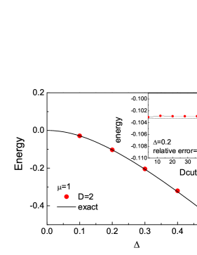
Figure 9: (Color online)Ground state energy per site as a function of $\Delta$ for fixed $\mu=1$. As a bench mark, we also plot the exact energy of the free fermion Hamiltonian. (Insert:) Relative error of ground state energy as a function of $D_{cut}$ for $\Delta=0.2$. $D_{cut}$ is the number of singular values kept in the Grassmann SVD decompositionVerstraete and Cirac (2004).

Although we get good results for the above simple example, it is not quite surprising since a trivial gapped fermion system only involves local physics. A much more challenging and interesting example is at $\mu=0$, in which case the low energy physics of the system is described by two Dirac cones in the first Brillouin zone(BZ). Actually, up to a particle-hole transformation on one sublattice, the above fermion paring Hamiltonian is equivalent to the fermion hopping Hamiltonian that describes the novel physics in graphene(the spin less version) where low energy electrons deserve a Dirac like dispersion. In Fig. 10, we plot the ground state energy as a function of $D_{cut}$ for inner dimensions $D=2$ and $D=4$. In this case, the $D=2$ approach only gives very poor results comparing to the gapped case. However, when we increase the inner dimension to $D=4$, we find that the ground state energy agrees pretty well with the exact one, with a relative error of $0.6\%$. Another interesting feature is that such a critical system would require a much larger $D_{cut}$(around $D_{cut}=70$ for $D=4$.) for the convergence of the GTERG algorithm. Later, we will discuss a possible improvement for the GTERG algorithm, which allows us to access much larger inner dimension $D$.

Finally, we would like to make some comments and discussions about the above results:

(a) Although a gapless fermion system with Dirac cones is critical, it does not violate the area law because it only contains zero dimensional Fermi surfaces.

(b) The good agreement in ground state energy does not imply the good agreement in long range correlations. Indeed, our conjecture is that for any finite $D$, the variational wave function we derive may always be associated with a finite correlation length which scales polynomially in $D$. We note that an interesting critical fPEPS state with finite inner dimension $D=2$ was proposed in Ref.Kraus et al. (2009), however, that model is different from our case since the Dirac cones in that model contain a quadratic dispersion along some directions in the first BZ.

(c) Although the GTPS variational approach can not describe the above system with finite inner dimension $D$, the variational results will still be very useful. From the numerical side, we can apply both finite $D$ and finite size scalings to estimate the physical quantities in the infinite $D$ and infinite size limit. From the analytic side, the finite correlation length corresponds to a finite gap in the system, which is known as Dirac mass term in the effective theoryPeskin (1995). In quantum field theory, a controlled calculation(without singularities in calculating correlation functions) can be performed by first taking the Dirac mass term to be finite and then pushing it to the zero limit.

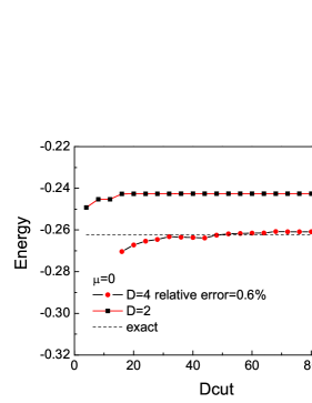
Figure 10: (Color online)Ground state energy per link as a function of $D_{cut}$ for fixed $\mu=0$ and $\Delta=0.25$. As a bench mark, we also plot the exact energy of the corresponding free fermion Hamiltonian.

III.4 An interacting fermion example

To this end, let us test an interacting fermion example with the following Hamiltonian:

$$H=-\sum_{\langle ij\rangle}\left(c_{i}^{\dagger}c_{j}+h.c.\right)-V\sum_{\langle ij\rangle}n_{i}n_{j}+\mu\sum_{i}(n_{i}-n_{f})$$ (51)

Such a Hamiltonian describes a spinless fermion system on honeycomb lattice with attractive interactions. In Fig. 11, we compare the ground state energy with exact diagonalization(ED) on $24$ sites and find a very good agreement for various fermion density $n_{f}$ at $V=0.5$. We use the GTPS ansatz with inner dimension $D=6$. We keep $D_{cut}$ up to $132$ to ensure the convergence of ground state energy. We also compute the superconducting order parameter on nearest neighbor(NN) bond and find a $p+ip$ pairing symmetry, which is consistent with the general argument that a spinless fermion system with attractive interactions supports $p+ip$ paring. In the insert of Fig. 11, we plot the amplitude of superconducting order parameter for various fermion densities. In Table 1, we show the phase shift of superconducting order parameters along three primary directions of honeycomb lattice.

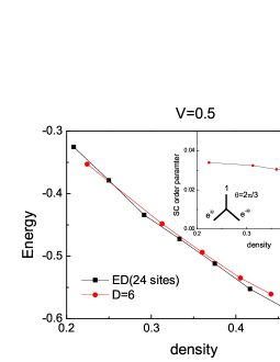
Figure 11: A comparison of the ground state energy per link as a function of electron density for spinless fermion on honeycomb lattice with attractive interactions.

Doping	$n_{f}=0.224$	$n_{f}=0.313$	$n_{f}=0.36$
$\Delta^{SC}_{a}/\Delta^{SC}_{b}$	(-0.4996,0.8656)	(-0.4995,0.8657)	(-0.4995,-0.8656)
$\Delta^{SC}_{b}/\Delta^{SC}_{c}$	(-0.5005,0.8660)	(-0.5006,0.8659)	(-0.5006,-0.8659)
$\Delta^{SC}_{c}/\Delta^{SC}_{a}$	(-0.4999,0.8664)	(-0.4999,0.8665)	(-0.4999,-0.8666)

Table 1: The phase shift of superconducting order parameter along three primary directions on honeycomb lattice.

IV Possible improvements of the GTERG approach

In this section, we will discuss possible improvements for the TERG algorithm and its Grassmann generalization. Again, let us start from the usual TPS case. Its Grassmann generalization would be straightforward by replacing the complex number valued tensors with those Grassmann valued tensors. We notice that the simple SVD method used in the TERG algorithm actually implies the following cost function:

$$f_{\rm{SVD}}=||\mathbb{T}-\mathbb{S}\cdot\mathbb{S}^{\prime}||,$$ (52)

where the rank four double tensor $\mathbb{T}$ is defined as $\mathbb{T}_{A}\cdot\mathbb{T}_{B}$ and $\cdot$ means summing over indices for the connected link, as seen in Fig.12 (a).(Actually it is the inner product of two vectors if we interpolate $\mathbb{T}_{A(B)}$ as $D^{6}$ dimensional vectors, where $D$ is the inner dimension of the TPS.) $||\cdots||$ is the usual $2$-norm of a vector. (The rank $4$ tensor $\mathbb{T}$ and rank $3$ tensors $\mathbb{S},\mathbb{S}^{\prime}$ can be viewed as $D^{8}$ and $D^{6}$ dimensional vectors.) Such a cost function only minimizes the $2$-norm of local error $\delta\mathbb{T}=\mathbb{T}-\mathbb{S}\cdot\mathbb{S}^{\prime}$ for a given cut-off dimension $D_{cut}$(the dimensional of the link shared by $\mathbb{S}$ and $\mathbb{S}^{\prime}$) and could not be the optimal one for minimizing global error. To figure out the optimal cost function, let us divide the system into large patches, as seen in Fig.13. If we trace out all the internal indices inside the patch, we can derive a rank $L$($L$ is the number of sites on the boundary of the patch) tensor $\mathbb{T}^{\prime}$ for the patch and the norm of TPS can be represented as the tensor trace of the new double tensors $\mathbb{T}^{\prime}$. When we perform the TERG algorithm and replace $\mathbb{T}$ by $\mathbb{S}\cdot\mathbb{S}^{\prime}$, we aim at making a small error for the double tensor $\mathbb{T}^{\prime}$.

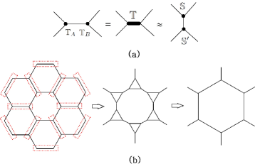
Figure 12: (Color online)(a) A graphic representation for $\mathbb{T}=\mathbb{T}_{A}\cdot\mathbb{T}_{B}$ and $\mathbb{T}\sim\mathbb{S}\cdot\mathbb{S}^{\prime}$. The symbol $\cdot$ here means sum over the indices for the shared link for two connected tensors. (b)A schematic plot for the TERG scheme on honeycomb lattice. The first step is approximate while the second step is exact.

Now it is clear why the simple SVD method that minimizes local errors could not approximate the patch double tensor $\mathbb{T}^{\prime}$ in an optimal way. Let us rewrite $\mathbb{T}^{\prime}$ as $\mathbb{T}^{\prime}=\mathbb{E}\cdot\mathbb{T}$.(Notice that here we regard the rank $L$ double tensor $\mathbb{T}^{\prime}$ as a $D^{2L}$ dimensional vector, the rank $4$ double tensor $\mathbb{T}$ as a $D^{8}$ dimensional vector and the rank $L+4$ double tensor $\mathbb{E}$ as a $D^{2L}$ by $D^{8}$ matrix.) The double tensor $\mathbb{E}$ is called environment tensor. The cost function which provides the best approximation for $\mathbb{T}^{\prime}$ can be represented as:

$$f=||\mathbb{E}\cdot\left(\mathbb{T}-\mathbb{S}\cdot\mathbb{S}^{\prime}\right)||$$ (53)

Again, $\cdot$ means the vector inner product and $||\cdots||$ means the usual $2$-norm. Comparing to the simple SVD method, the environment tensor gives a complex weight for each component of the local error $\delta\mathbb{T}$. Notice that the cost function proposed here is very different from the one in Ref.Z.Y. et al. (2008-2010), which aims at minimizing ${\rm{Tr}}\left(\mathbb{E}\cdot\mathbb{T}\right)$.

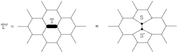
Figure 13: A schematic plot for the patch double tensor $\mathbb{T}^{\prime}$. The global cost function aims at finding the best way to minimize the error for the above patch double tensor.

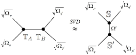
Figure 14: A graphic representation for the first step of the weighted TERG algorithm.

Although the environment tensor $\mathbb{E}$ is conceptually useful, it is impossible to compute this rank $L+4$ tensor when the patch size becomes very large. Nevertheless, we can derive a simplified environment through the simplified time evolution algorithm. The key step is also based on the conjecture that the rank $8$ tensor $\mathbb{E}^{\dagger}\cdot\mathbb{E}$ can be factorized into a product form:

$$\left(\mathbb{E}^{\dagger}\cdot\mathbb{E}\right)_{pqp^{\prime}q^{\prime};\bar{p}\bar{q}\bar{p}^{\prime}\bar{q}^{\prime}}=\Omega_{p}^{y}\Omega_{q}^{z}\Omega_{p^{\prime}}^{y}\Omega_{q^{\prime}}^{z}\delta_{p\bar{p}}\delta_{q\bar{q}}\delta_{p^{\prime}\bar{p}^{\prime}}\delta_{p^{\prime}\bar{p}^{\prime}},$$ (54)

where $p=(b,\bar{b})$,$q=(c,\bar{c})$ are the double indices. For any converged $T_{A}$ and $T_{B}$ from the simplified time evolution algorithm with converged weight vectors ${\Lambda^{*}}^{\alpha}$, the weight vectors $\Omega^{\alpha}$ for double tensors $\mathbb{T}$ can be determined as:

$$\Omega_{p}^{y}={\Lambda^{*}}_{b}^{y}{\Lambda^{*}}_{\bar{b}}^{y},\Omega_{q}^{z}={\Lambda^{*}}_{c}^{z}{\Lambda^{*}}_{\bar{c}}^{z}.$$ (55)

The above conjecture for the environment is reasonable when the environment of $T^{m}$ can be approximated as a product form since $\mathbb{T}=\sum_{m}{\bar{T}^{m}}\otimes T^{m}$

Similar to the simplified time evolution algorithm, solving the optimal cost function in this case can be implemented by the SVD decomposition for matrix $\mathbb{M}$(see Fig. 14):

$$\mathbb{M}_{q^{\prime}p;qp^{\prime}}= \mathbb{T}_{pqp^{\prime}q^{\prime}}\sqrt{\Omega_{p}}\sqrt{\Omega_{q}}\sqrt{\Omega_{p^{\prime}}}\sqrt{\Omega_{q^{\prime}}}$$

$$\simeq \sum_{r=1}^{D_{cut}}U_{q^{\prime}p;r}V_{qp^{\prime};r}\Omega_{r}^{\prime}$$ (56)

Then the rank $3$ double tensors $\mathbb{S}$ and $\mathbb{S}^{\prime}$ can be determined as:

$$\mathbb{S}_{rq^{\prime}p} =\frac{\sqrt{\Omega_{r}^{\prime}}}{\sqrt{\Omega_{q^{\prime}}}\sqrt{\Omega_{p}}}U_{q^{\prime}p;r}$$

$$\mathbb{S}_{r^{\prime}qp^{\prime}}^{\prime} =\frac{\sqrt{\Omega_{r^{\prime}}^{\prime}}}{\sqrt{\Omega_{q}}\sqrt{\Omega_{p^{\prime}}}}V_{qp^{\prime};r^{\prime}}$$ (57)

Finally, the weight vector $\Omega^{x}$ for $x-link$ can be updated as $\Omega^{x}=\Omega^{\prime}$.

In general cases, the assumption Eq.(54) could not be true, however, as long as $\mathbb{E}_{\lambda;pqp^{\prime}q^{\prime}}/\sqrt{\Omega_{p}}\sqrt{\Omega_{q}}\sqrt{\Omega_{p^{\prime}}}\sqrt{\Omega_{q^{\prime}}}$ has a much more uniform distribution(up to proper normalization):

$$\left|\frac{\mathbb{E}_{\lambda;pqp^{\prime}q^{\prime}}}{\sqrt{\Omega_{p}}\sqrt{\Omega_{q}}\sqrt{\Omega_{p^{\prime}}}\sqrt{\Omega_{q^{\prime}}}}\right|\sim 1,$$ (58)

the above weighted TERG(wTERG) algorithm can still improve the accuracy for fixed $D_{cut}$ with the same cost. This is because the SVD method is the best truncation method if the environment has a random but uniform distribution.

By replacing the complex valued double tensors with Grassmann variable valued double tensors, all the above discussions will be valid for GTPS. However, the definition of the inner product $\cdot$ and the corresponding 2-norm $||\cdots||$ should also be generalized into their Grassmann version, which evolves the integration over Grassmann variables for the connected links with respect to the standard Grassmann metric. For example, the cost function of the GSVD method discussed in Ref.Gu et al. (2010) can be formally written as:

$$f_{\rm{GSVD}}=\delta\mathbb{T}^{f}\cdot{\delta\mathbb{T}^{f}}^{\dagger}=||\delta\mathbb{T}^{f}||=||\mathbb{T}^{f}-\mathbb{S}^{f}\cdot{\mathbb{S}^{\prime}}^{f}||,$$ (59)

To explain the meaning of the above expression more explicitly, we consider a simple case that $\mathbb{T}^{f}$ only contains one species of Grassmann variables. We can express $\mathbb{T}^{f}$ as:

$$\mathbb{T}^{f}_{pqp^{\prime}q^{\prime}}=\mathbb{T}_{pqp^{\prime}q^{\prime}}\left(\theta_{\beta}\right)^{N_{f}(p)}\left(\theta_{\gamma}\right)^{N_{f}(q)}\left(\theta_{\beta^{\prime}}\right)^{N_{f}(p^{\prime})}\left(\theta_{\gamma^{\prime}}\right)^{N_{f}(q^{\prime})},$$ (60)

where $\mathbb{T}_{pqp^{\prime}q^{\prime}}$ is the complex coefficient of the Grassmann number valued double tensor $\mathbb{T}^{f}_{pqp^{\prime}q^{\prime}}$ and $N_{f}(p)=\frac{P_{f}(p)+1}{2}$ is determined by the fermion parity of the inner index $p$. We notice that $\mathbb{T}_{pqp^{\prime}q^{\prime}}=\sum_{r}\mathbb{T}_{A;rpq}\mathbb{T}_{B;rp^{\prime}q^{\prime}}$ if we express the Grassmann number valued double tensors $\mathbb{T}_{A(B);rpq}^{f}$ on sublattice $A(B)$ as:

$$\mathbb{T}_{A(B);rpq}^{f}=\mathbb{T}_{A(B);rpq}\left(\theta_{\alpha}\right)^{N_{f}(r)}\left(\theta_{\beta}\right)^{N_{f}(p)}\left(\theta_{\gamma}\right)^{N_{f}(q)}$$ (61)

Similarly, we can express $\mathbb{S}^{f}$ and $\mathbb{S^{\prime}}^{f}$ as:

$$\mathbb{S}^{f}_{rq^{\prime}p} =\mathbb{S}_{rq^{\prime}p}\left(\theta_{\alpha}\right)^{N_{f}(r)}\left(\theta_{\gamma^{\prime}}\right)^{N_{f}(q^{\prime})}\left(\theta_{\beta}\right)^{N_{f}(p)}$$

$$\mathbb{S^{\prime}}^{f}_{r^{\prime}qp^{\prime}} =\mathbb{S^{\prime}}_{r^{\prime}qp^{\prime}}\left(\theta_{\alpha^{\prime}}\right)^{N_{f}(r^{\prime})}\left(\theta_{\gamma}\right)^{N_{f}(q)}\left(\theta_{\beta^{\prime}}\right)^{N_{f}(p^{\prime})}$$ (62)

Again, $\mathbb{S}_{rq^{\prime}p}$ and $\mathbb{S^{\prime}}_{r^{\prime}qp^{\prime}}$ are the complex valued coefficients. Recall the definition of the standard Grassmann metric $\mathbf{g}_{rr^{\prime}}$:

$$\mathbf{g}_{rr^{\prime}}=\delta_{rr^{\prime}}\left(\mathrm{d}\theta_{\alpha}\right)^{N_{f}(r)}\left(\mathrm{d}\theta_{\alpha^{\prime}}\right)^{N_{f}(r^{\prime})},$$ (63)

the inner product $\mathbb{S}^{f}\cdot\mathbb{S^{\prime}}^{f}$ explicitly means:

$$\left(\mathbb{S}^{f}\cdot\mathbb{S^{\prime}}^{f}\right)_{pqp^{\prime}q^{\prime}} =\sum_{rr^{\prime}}\int\mathbf{g}_{rr^{\prime}}\mathbb{S}_{rq^{\prime}p}\mathbb{S^{\prime}}_{r^{\prime}qp^{\prime}}\left(\theta_{\alpha}\right)^{N_{f}(r)}\left(\theta_{\gamma^{\prime}}\right)^{N_{f}(q^{\prime})}\left(\theta_{\beta}\right)^{N_{f}(p)}\left(\theta_{\alpha^{\prime}}\right)^{N_{f}(r^{\prime})}\left(\theta_{\gamma}\right)^{N_{f}(q)}\left(\theta_{\beta^{\prime}}\right)^{N_{f}(p^{\prime})}$$

$$=\sum_{r}\mathbb{S}_{rq^{\prime}p}\mathbb{S^{\prime}}_{r^{\prime}qp^{\prime}}\left(\theta_{\gamma^{\prime}}\right)^{N_{f}(q^{\prime})}\left(\theta_{\beta}\right)^{N_{f}(p)}\left(\theta_{\gamma}\right)^{N_{f}(q)}\left(\theta_{\beta^{\prime}}\right)^{N_{f}(p^{\prime})}.$$ (64)

Thus, we have:

$$\delta\mathbb{T}^{f}_{pqp^{\prime}q^{\prime}}=\delta\mathbb{T}_{pqp^{\prime}q^{\prime}}\left(\theta_{\gamma^{\prime}}\right)^{N_{f}(q^{\prime})}\left(\theta_{\beta}\right)^{N_{f}(p)}\left(\theta_{\gamma}\right)^{N_{f}(q)}\left(\theta_{\beta^{\prime}}\right)^{N_{f}(p^{\prime})},$$ (65)

with

$$\delta\mathbb{T}_{pqp^{\prime}q^{\prime}} =\mathbb{T}_{pqp^{\prime}q^{\prime}}(-)^{N_{f}(p^{\prime})}-\sum_{r}\mathbb{S}_{rq^{\prime}p}\mathbb{S^{\prime}}_{rqp^{\prime}}$$

$$=\mathbb{T}_{pqp^{\prime}q^{\prime}}^{\prime}-\sum_{r}\mathbb{S}_{rq^{\prime}p}\mathbb{S^{\prime}}_{rqp^{\prime}}$$ (66)

Now it is clear that up to a sign twist, the GSVD cost function is equivalent to the cost function of its complex coefficient tensors:

$$f_{GSVD}=||\delta\mathbb{T}^{f}||=||\delta\mathbb{T}||=||\mathbb{T}^{\prime}-\mathbb{S}\cdot{\mathbb{S}^{\prime}}||$$ (67)

Explicitly the same as in the TERG case, the best approximation for a given $D_{cut}$ is nothing but the SVD decomposition for the coefficient tensor $\mathbb{T}^{\prime}$.(If we view $\mathbb{T}_{pqp^{\prime}q^{\prime}}^{\prime}$ as a matrix $\mathbb{M}_{q^{\prime}p;qp^{\prime}}=\mathbb{T}_{pqp^{\prime}q^{\prime}}^{\prime}\simeq\sum_{r=1}^{D_{cut}}\mathbb{S}_{rp^{\prime}q}\mathbb{S^{\prime}}_{rqp^{\prime}}$.) On the other hand, as already having been discussed in Ref.Gu et al. (2010), the constraint Eq. (5) of GTPS implies that their double tensors contain even number of Grassmann numbers. As a result, $\mathbb{M}$ is block diagonalized and the index $r$ will have a definite parity $P^{f}(r)=P^{f}(p)P^{f}(q)=P^{f}(p^{\prime})P^{f}(q^{\prime})$. We notice that the novel sign factor $(-)^{N_{f}(p^{\prime})}$ here arises from the anti-commuting nature of the Grassmann variables and will encode the fermion statistics. The second RG step remains the same as in GTERG and a similar novel sign factor will also emerge there.

All the above discussion will still be correct if the inner index of the double tensor $\mathbb{T}^{f}$ contains multiple species of Grassmann variables. Indeed, starting from the standard GTPS, the double tensor $\mathbb{T}^{f}$ in the first RG step will contain two species of Grassmann variables. This is because $\mathbb{T}^{f}_{A(B)}=\sum_{m}\mathbf{\bar{T}}_{A(B)}^{m}\otimes\mathbf{T}_{A(B)}^{m}$ and $\mathbb{T}^{f}=\mathbb{T}^{f}_{A}\cdot\mathbb{T}^{f}_{B}$. In the second and latter RG steps, $\mathbb{T}^{f}_{A(B)}$ will only contain one species of Grassmann variables.

The discussion for the environment effect will be in a similar way. Especially, if we use some weighting factors to approximately represent the environment effect, the coefficient tensors $\mathbb{S},\mathbb{S}^{\prime}$ will take the same form as in the usual TPS case. However, an important sign factor should be included when we define the matrix $\mathbb{M}$. Again,the environment weight for the first step is determined by the time evolution algorithm of GTPS. Same as in the bosonic case, the singular value obtained from the GSVD would perform as the environment weight for the next RG step.

In Fig. 15, we implement the above algorithm to the free fermion Hamiltonian Eq.(50) at critical point($\mu=0$). We see an important improvement that the ground state energy decreases when increasing $D_{cut}$ and is strictly above the exact energy, unlike the simple GTERG approach, which can overestimate the ground state energy for small $D_{cut}$. However, for large enough $D_{cut}$, the two approaches converge to the same values, as expected. We further use the new algorithm to study the critical model with larger inner dimension $D$. Up to $D=6$, we find that the ground state energy from the GTPS approach is almost the same as the exact one(relative error $\sim 0.1\%$).

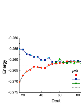
Figure 15: A comparison of the ground state energy per link as a function of $D_{cut}$ at $\mu=0$ and $\Delta=0.25$ . By introducing the environment weight in the GTERG method, an important improvement is that the ground state energy is always above the exact value, which is very important for variational approach

.

V Summary

In this paper, we first derive a standard form of GTPS that only contains one species of Grassmann variables for each inner index and significantly simplifies the representations in our numerical calculations. Based on the fermion coherent state representation, we further generalize the imaginary time evolution algorithms into fermion systems. We study a simple free fermion example on honeycomb lattice, including both off-critical and critical cases to test our new algorithms. Finally, we discuss the importance of the environment effect of the TERG/GTERG method and present a simple improvement by introducing proper environment weights.

Although the simple time evolution algorithm discussed here is not generic enough, it has already allowed us to study many interesting and important models, such as the Hubbard/$t-J$ model, whose ground state is believed to be a superconductor. The evidence for the existence of superconductivity in these models based on the GTPS algorithm will be discussed and bench marked with other methods elsewhereGu (2011). Of course, the generic algorithm is also very important and desired, especially for those systems with topological order. Actually, the general discussions in Section II have already made some progress along this direction, but not efficient and stable enough at this stage.

On the other hand, further improving the efficiency of contracting (Grassmanna) tensor net is also very important. Although the GTERG/TERG algorithm provides us promising results in many cases, it is still not efficient enough since the algorithm is not easy to be parallelized. Recently, a novel idea of combining the concept of renormalization and Monte Carlo(MC)Ling et al. (2010) has made great success for boson/spin systems, it would be very natural to generalize it into fermion/electron systems based on the Grassmann variable representations.

We would like to thank F.Verstrate, J.I.Cirac and X.G. Wen for very helpful discussions. We especially thank D.N. Sheng for providing the ED data. This work is supported in part by NSF Grant No. NSFPHY05-51164

References

- Gu et al. (2010) Z.-C. Gu, F. Verstraete, and X.-G. Wen, (2010), eprint arXiv:cond-mat/1004.2563.
- Laughlin (1983) R. B. Laughlin, Phys. Rev. Lett. 50, 1395 (1983).
- Wen and Niu (1990) X.-G. Wen,and Qian Niu, Phys. Rev. B 41, 9377 (1990).
- Anderson (1987) P. W. Anderson Science 235, 1196 (1987).
- Gros (1988) C. Gros Phys. Rev. B 38, 931 (1988).
- Lee, Nagaosa and Wen (2006) For a review, see P. A. Lee, N. Nagaosa and X.-G. Wen, Phys. Mod. Phys. 78, 17 (2006).
- Wen (2002) X.-G. Wen, Phys. Rev. B 65, 165113 (2002).
- Ying, Michael, Patrick and Wen (1983) Ying Ran, Michael Hermele, P. A. Nagaosa and X.-G. Wen, Phys. Rev. Lett. 98, 117205 (2007).
- Wen (1999) X.-G. Wen, Phys. Rev. B 60, 8827 (1999).
- Gu et al. (2009) Z.-C. Gu, M. Levin, B. Swingle,and X.-G. Wen, Phys. Rev. B 79, 085118 (2009).
- Buerschaper et al. (2009) O. Buerschaper, M. Aguado,and G. Vidal, Phys. Rev. B 79, 085119 (2009).
- Levin et al. (2009) M. Levin,and X.-G. Wen, Phys. Rev. B 71, 045110 (2005).
- Gu et al. (2010) Z.-C. Gu, Z. Wang, and X.-G. Wen, (2010), eprint arXiv:cond-mat/1010.1517.
- Dubail et al (2010) J. Dubail,and N. Read, (2013), eprint arXiv:cond-mat/1307.7726.
- T. B. et al (2010) T. B. Wahl, H. H. Tu, N. Schuch,and J. I. Cirac, (2013), eprint arXiv:cond-mat/1308.0316.
- Bri et al. (2011) B. Bri,and N. R. Cooper, Phys. Rev. Lett. 106, 156401 (2011).
- Frank et al. (2008/2009) F. Verstraete, J. I. Cirac, and V. Murg, Adv. Phys. 57, 143 (2008); J. I. Cirac, and F. Verstraete, J. Phys. A: Math. Theor. 42, 504 (2009).
- Verstraete and Cirac (2004) F. Verstraete and J. I. Cirac (2004), eprint arXiv:cond-mat/0407066.
- Kraus et al. (2009) C. V. Kraus, N. Schuch, F. Verstraete, and J. I. Cirac Phys. Rev. A 81, 052338 (2010).
- Barthel et al. (2009) T. Barthel, C. Pineda, and J. Eisert, Phys. Rev. A 80, 042333 (2009).
- Corboz et al. (2009) P. Corboz, R. Orus, B. Bauer,and G. vidal, Phys. Rev. B 81, 165104 (2010).
- Iztok et al. (2010) Iztok Pizorn, and Frank Verstraete, Phys. Rev. B 81, 245110 (2010).
- Q.Q.Shi et al. (2009) Q. Q. Shi, S. H. Li, J. H. Zhao, and H. Q. Zhou, (2009), eprint arXiv:cond-mat/0907.5520.
- Corboz et al. (2011) P. Corboz, J. Jordan,and G. Vidal, Phys. Rev. B 82, 245119 (2010).
- Corboz et al. (2011) P. Corboz, S. R. White, G. Vidal,and M. Troyer, Phys. Rev. B 84, 041108 (2011).
- Schuch et al. (2007) N. Schuch, M. M. Wolf, F. Verstraete, and J. I. Cirac, Physical Review Letters 98, 140506 (2007).
- Murg et al. (2007) V. Murg, F. Verstraete, and J. I. Cirac, Phys. Rev. A 75, 033605 (2007).
- Jordan et al. (2008) J. Jordan, R. Orus, G. Vidal, F. Verstraete, and J. I. Cirac, Physical Review Letters 101, 250602 (2008).
- Murg et al. (2009) Roman Orus, and Guifre Vidal, Phys. Rev. B 80, 094403 (2009).
- Levin and Nave (2007) M. Levin and C. P. Nave, Phys. Rev. Lett. 99, 120601 (2007).
- Gu et al. (2008) Z.-C. Gu, M. Levin, and X.-G. Wen, Phys. Rev. B 78, 205116 (2008).
- Jiang et al. (2008) H. C. Jiang, Z. Y. Weng, and T. Xiang, Phys. Rev. Lett. 101, 090603 (2008).
- Z.Y. et al. (2008-2010) Z. Y. Xie, H. C. Jiang, Q. N. Chen, Z. Y. Weng, and T. Xiang, Phys. Rev. Lett. 103, 160601 (2009); H. H. Zhao, Z. Y. Xie, Q. N. Chen, Z. C. Wei, J. W. Cai,and T. Xiang, Phys. Rev. B 81, 174411 (2010).
- Xie et al. (2010) Xie Chen, Z.-C. Gu, and X.-G. Wen, Phys. Rev. B 82, 155138 (2010).
- Ling et al. (2010) Ling Wang, Iztok Piorn, and Frank Verstraete, Phys. Rev. B 83, 134421 (2011).
- Vidal et al. (2007) G. Vidal, Phys. Rev. Lett. 98, 070201 (2007).
- Peskin (1995) M. E. Peskin, and D. V. Schroeder, An introduction to quantum field theory (Westview Press, 1995).
- Gu (2011) Z.-C. Gu, H.-C. Jiang, D.-N. Sheng, Hong Yao, Leon Balents, and X.-G. Wen, (2011),eprint arXiv:cond-mat/1110.1183.