The quiet Sun average Doppler shift of coronal lines up to 2 MK

Abstract

Context. The average Doppler shift shown by spectral lines formed from the chromosphere to the corona reveals important information on the mass and energy balance of the solar atmosphere, providing an important observational constraint to any models of the solar corona. Previous spectroscopic observations of vacuum ultra-violet (VUV) lines have revealed a persistent average wavelength shift of lines formed at temperatures up to 1 MK. At higher temperatures, the behaviour is still essentially unknown.

Aims. Here we analyse combined SUMER (Solar Ultraviolet Measurements of Emitted Radiation)/SoHO (Solar and Heliospheric Observatory) and EIS (EUV Imaging Spectrometer)/Hinode observations of the quiet Sun around disk centre to determine, for the first time, the average Doppler shift of several spectral lines formed between 1 and 2 MK, where the largest part of the quiet coronal emission is formed.

Methods. The measurements are based on a novel technique applied to EIS spectra to measure the difference in Doppler shift between lines formed at different temperatures. Simultaneous wavelength-calibrated SUMER spectra allow establishing the absolute value at the reference temperature of $T\approx$ 1 MK.

Results. The average line shifts at 1 MK$\leavevmode\nobreak\ <T<1.8$ MK are modestly, but clearly bluer than those observed at 1 MK. By accepting an average blue shift of about $(-1.8\pm 0.6)\leavevmode\nobreak\ \rm km\leavevmode\nobreak\ s^{-1}$ at 1 MK (as provided by SUMER measurements), this translates into a maximum Doppler shift of $(-4.4\pm 2.2)\leavevmode\nobreak\ \rm km\leavevmode\nobreak\ s^{-1}$ around 1.8 MK. The measured value appears to decrease to about $(-1.3\pm 2.6)\leavevmode\nobreak\ \rm km\leavevmode\nobreak\ s^{-1}$ at the Fe xv formation temperature of 2.1 MK.

Conclusions. The measured average Doppler shift between 0.01 and 2.1 MK, for which we provide a parametrisation, appears to be qualitatively and roughly quantitatively consistent with what foreseen by 3-D coronal models where heating is produced by dissipation of currents induced by photospheric motions and by reconnection with emerging magnetic flux.

1 Introduction

Ultraviolet observations of the Sun near disk centre show a systematic net red shift of emission lines from the transition region (TR). Several vacuum ultra-violet (VUV: 16 to 200 nm) spectrometers with different spatial resolutions such as HRTS and those flown on Skylab, OSO 8, and SMM have revealed this phenomenon since the 1970s (e.g., Doschek et al. 1976; Hassler et al. 1991; Brekke 1993; Achour et al. 1995). Systematic red shifts have also been observed in spectra of late type stars (e.g., Ayres et al. 1988; Wood et al. 1996; Pagano et al. 2004), indicating that this phenomenon is not unique to the Sun.

In these earlier investigations (before the launch of SoHO in 1995), the magnitude of the red shift was found to increase with temperature, reaching a maximum at $T=0.1$ MK and then decreasing toward higher temperatures. However, these observations were, with few exceptions, restricted to temperatures below 0.2 MK.

Observations from SOHO extended the observable temperature range up to about 1 MK. In the quiet Sun near disk centre, Doppler shifts in the range of 10 to 16 km s^-1 were confirmed in lines formed from $T=$ 0.1 MK to 0.25 MK (e.g., Brekke et al. 1997; Chae et al. 1998; Peter & Judge 1999; Teriaca et al. 1999a).

At higher temperatures (0.6 to 1 MK), the interpretation of the measurements proved to be more controversial. Brekke et al. (1997) and Chae et al. (1998) reported red shifted (downward) average Doppler velocities of 6.0 and 3.8 km s^-1 for Mg x $\lambda$625 ($T=$ 1.0 MK) and of 5.0 and 5.3 km s^-1 for Ne viii $\lambda$770 ($T=$ 0.63 MK). These Doppler velocities were derived by using the reference rest wavelengths of 770.409 Å and 624.950 Å compiled by Kelly (1987) (based on solar observations, see discussion in Peter & Judge 1999), affected by high uncertainties (high in relation to the Doppler shifts under discussion).

Peter & Judge (1999) and Dammasch et al. (1999a, b) took another approach and obtained accurate rest wavelengths for the above lines by assuming that the average Doppler velocity is around zero above the solar limb (motions along the line of sight cancel out on average in an optically thin plasma). With these new rest wavelengths, average blue shifts of a few km s^-1 were found for both lines near disk centre (Peter 1999; Peter & Judge 1999; Dammasch et al. 1999a, b; Teriaca et al. 1999a). These results suggest that there is a transition from red to blue shifts above 0.5 MK. This transition is an important observational constraint to distinguish between different models of the solar transition region.

Several hypotheses to explain the observed shifts of TR and coronal lines have been discussed in the literature. Since spicules carry an upward mass flux about 100 times larger than carried out by the global solar wind, it was suggested that the TR emission is dominated by downflowing, cooling plasma injected into the corona by spicules (Pneuman & Kopp 1978; Athay & Holzer 1982; Athay 1984). Lack of direct observational evidence (Withbroe 1983) and failure of theoretical models to reproduce observations (Mariska 1987) have led to a general dismissal of this hypothesis. However, recent analysis of spectroscopic and imaging VUV data with high sensitivity and spatial resolution has revived interest in the role of spicules in the mass and energy balance of the solar corona (e.g., De Pontieu et al. 2009; McIntosh & De Pontieu 2009a, b; De Pontieu et al. 2011).

Much effort has also been put into modelling the effect of energy deposition (e.g., mimicking the effect of magnetic reconnection in different regions of the solar atmosphere) on line profiles. Cheng (1992) showed that impulsive energy release in the photosphere generates a shock train that propagates upward and lifts and heats the chromosphere and TR, giving rise to an average downward material velocity. However, Hansteen & Wikstol (1994) demonstrated that, contrary to observations, the resulting line emission is nevertheless blue shifted. Instead of upward propagating waves, Hansteen (1993) interpreted the observed red shift as caused by downward propagating acoustic waves. Nanoflares releasing relatively small amounts of energy near the top of the magnetic loops give rise to disturbances running downward along the loop legs. In a later study Hansteen et al. (1997) included the effect of reflection in the chromosphere of downward propagating MHD waves. This increases the red shifts in the TR, although coronal blue shifts become too high. An investigation by Judge et al. (1998) lends observational support to the picture of downward running waves or disturbances.

More generally, models of energy deposition at TR temperatures in 1-D loops have managed to reproduce the observed TR red shifts and low corona blue shifts relatively well (Teriaca et al. 1999b; Spadaro et al. 2006).

Recently, three-dimensional (3-D) comprehensive numerical models of the solar atmosphere (from photosphere to corona) have been developed. In the model described by Peter et al. (2004, 2006), coronal heating is caused by the Joule dissipation of the currents that are produced when magnetic field is stressed and braided by photospheric motions. This model does produce red shifts at TR temperatures but also in the low corona, where blue shifts are instead observed. Hansteen et al. (2010) extended that work and added the effects of episodic injections of emerging magnetic flux that reconnects with the existing field. Rapid, episodic heating of the upper chromospheric plasma to coronal temperatures naturally produces downflows in TR lines and slight upflows in low coronal lines. As suggested by the authors, the localised heating events occurring in the chromosphere generate high-speed flows in a wide range of temperatures that may be related to the high-speed upflows that have been deduced from significant blueward asymmetries in EIS/Hinode observations of many TR and coronal lines (Hara et al. 2008; De Pontieu et al. 2009; McIntosh & De Pontieu 2009a, b) that have been linked to spicules (i.e., De Pontieu et al. 2011).

With the launch of the Extreme Ultraviolet Imaging Spectrograph (EIS, Culhane et al. 2007; Korendyke et al. 2006) aboard Hinode, high spectral and spatial resolution observations in intense spectral lines formed at temperatures above 1 MK have finally become available. In this work, by using combined SUMER (Solar Ultraviolet Measurement of Emitted Radiation)/SoHO and EIS/Hinode observations of the quiet Sun and a novel technique, we have characterised the Doppler shift versus temperature behaviour up to 2.1 MK.

In Section 2, we describe the SUMER data and their analysis. In addition, we determine the Doppler velocity for N v $\lambda$1238, N v $\lambda$1242, and Mg x $\lambda$625 lines in the quiet Sun near disk centre. We also discuss the EIS/Hinode data, their analysis, and their co-alignment with the SUMER data. In Section 3 we present our method to measure the average Doppler velocity of hot coronal ions using SUMER/SoHO and EIS/Hinode data. Section 4 and 5 present results and conclusions, respectively.

2 Observations and data analysis

Spectra of a quiet region near disk centre were taken on 6 April 2007 from 00:00 to 06:00 UTC during the first EIS-SUMER campaign (HOP 3). Figure 1 shows the Sun on the day of observations as recorded by the Extreme Ultraviolet Telescope (EIT, Delaboudinière et al. 1995) aboard SOHO. The quiet Sun areas observed by SUMER and EIS are visible near disk centre.

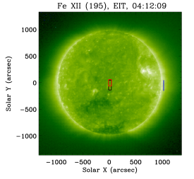
Figure 1: Fe xii 195 Å EIT image. The areas observed on the disk by SUMER (smaller red box) and EIS (larger black box) are shown. They are located near disk centre in a quiet region. The off-limb pointing of the EIS slit (about 50 $\arcsec$ above the west limb) is indicated by the vertical black line.

2.1 SUMER data: Doppler shift of Mg x and N v

SUMER is a normal incidence spectrograph operating over the wavelength range 450 Å to 1610 Å. It is a powerful UV instrument capable of making measurements of bulk motions in the chromosphere, TR, and low corona with a spatial resolution of 1$\arcsec$ across and 2$\arcsec$ along the slit and a spectral scale of $\approx$ 43 mÅ/pix at 1240 Å (first order) (Wilhelm et al. 1995; Lemaire et al. 1997), which is high enough to measure line shifts down to 1 km s^-1. Spectral images have been decompressed, wavelength-reversed, corrected for dead time, flat-field, and detector electronic distortion.

Since SUMER does not have an on-board calibration source, we derive the wavelength scale by using a set of chromospheric lines assumed to have negligible or low average Doppler shift on the quiet Sun. In short, calibrating takes three main steps:

1. Identify the spectral lines by using the preliminary wavelength scale.

2. Find the exact pixel position of the lines by fitting Gaussian curves.

3. Perform a polynomial fit to find the dispersion relation.

To perform an accurate calibration we have to choose fairly strong and unblended lines from neutral and singly ionised atoms. For instance, Si i, S i, and C i transitions, occurring at temperatures between 6500 and 10000 K, are very suitable calibration lines, since lines formed at such temperatures show, on average, no substantial Doppler shifts (Samain 1991).

The SUMER data analysed here consist of a raster formed by 40 slit positions with a step size of $1.87\arcsec$ taken between 03:26 and 04:31 UTC by exposing through the $1\arcsec\times 120\arcsec$ slit for 100 s. Recorded spectra cover the 1210 Å to 1270 Å range containing the N v lines at 1238.8 Å and 1242.8 Å (log($T$/[K])=5.24) and the Mg x line at 625 Å (log($T$/[K])=6.00). The above spectral range also contains a forbidden line of Fe xii at 1242 Å that would be ideal for a combined study with EIS. However, on the quiet Sun this line is weak and blended with chromospheric lines from Ca ii and S i (see Dammasch et al. 1999a) and, for this reason, it is not possible to derive its average Doppler shift with the accuracy needed for our study.

After checking that there are no significant instrumental drifts in the position of the spectral lines (either along the slit either in time across the raster) we have obtained a high signal to noise spectrum to be calibrated in wavelength. We have selected ten suitable reference lines in the part of the spectrum which contains the N v lines. A first-order polynomial fit of their positions in pixels versus their laboratory wavelengths, leaves residuals of less than $\pm$ 0.2 pixels (less than 2 km s^-1, see Fig. 2).

For the part of the spectrum containing the Mg x line, we have selected nine suitable reference lines. If we use a first-order polynomial fit to the line positions, the residuals up to $\pm$ 0.6 pixels (top panel of Fig. 3). The residuals clearly show the need for a second-order polynomial fit that yields residuals of $\pm$ 0.05 pixels (bottom panel of Fig. 3). The need for the higher order fit comes most likely from residuals in the correction of the electronic distortion of the detector image.

From the above analysis, for the N v $\lambda$1238 and $\lambda$1242 lines we find net red shifts of (9.9 $\pm$ 0.6) km s^-1 and (12.1 $\pm$ 0.6) km s^-1 by assuming the rest wavelengths to be 1238.800 Å and 1242.778 Å (Edlén 1934). These velocities agree with those from lines formed at similar temperatures reported in the literature (e.g., Brekke et al. 1997; Chae et al. 1998; Peter & Judge 1999; Teriaca et al. 1999a).

In the case of the Mg x $\lambda$625 line (observed in the second-order of diffraction), we use 624.967 Å  as rest wavelength (average between the values of (624.965 $\pm$ 0.003) Å (Dammasch et al. 1999a) and (624.968 $\pm$ 0.007) Å (Peter & Judge 1999)), obtaining a Doppler velocity of ($-1.8\pm 0.6$) km s^-1 (Table 1). With the above rest wavelength, the Doppler shifts measured in Mg x by Brekke et al. (1997) and Chae et al. (1998) would result in velocities of about 0 km s${}^{-}1$ and $-2$ km s${}^{-}1$, respectively.

Brekke et al. (1997) discuss a possible blend in the red wing of the Mg x $\lambda$625 line with a first-order Si ii 1250.089 Å line and conclud that it has a negligible effect on the derived line shifts in spectra taken on the KBr-coated part of the SUMER detector. Teriaca et al. (2002) also discuss the relevance of blending from first-order lines to the Mg x line in the quiet Sun, concluding that they account for about 10% to 15% of the signal in the observed profile when observed on KBr (mostly from the Si ii 1250.089 Å line) and to 1% to 2% when observed on the uncoated detector (due to the low sensitivity to first-order lines with respect to the KBr-coated parts). Since our observations were obtained on the uncoated part of the SUMER detector, we consider blends from first-order lines as entirely negligible.

Blends from second-order lines such as S x 624.70 Å, O iv 624.617 Å, and 625.130 Å are potentially more dangerous. However, these lines are far enough from the centre of the Mg x line and would produce detectable “shoulders” in the observed profile. Moreover, constrained double Gaussian fits show no significant improvement in line fitting over fits with a single Gaussian. This speaks against significant blending in the Mg x $\lambda$625 line also from second-order lines.

Table 1: Doppler velocity of N v and Mg x lines:

ions	rest wavelength	$v$	$\delta v$
(log ($T$/[K]))	[Å]	[km s-1]	[km s-1]
N v (5.24)	1238.800	9.9	0.6
N v (5.24)	1242.778	12.1	0.6
Mg x (6.00)	624.967	-1.8	0.6

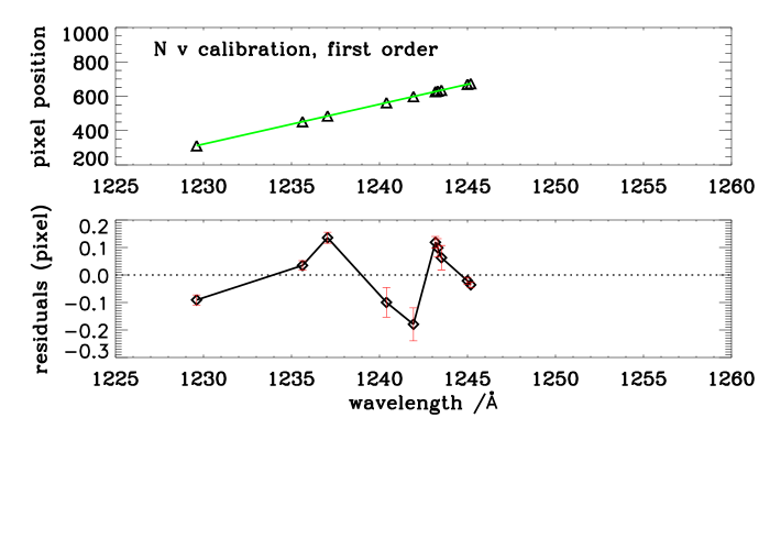
Figure 2: Upper panel: first-order polynomial fit to pixel positions versus rest wavelengths of 10 suitable reference lines around the N v lines. Lower panel: fit residuals are under 0.2 pixels (less than 2 km s^-1).

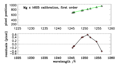
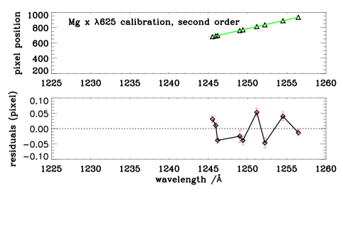
Figure 3: Top pair of panels: first-order polynomial fit to pixel positions versus rest wavelengths of 9 suitable reference lines around the Mg x lines. Residuals are large, up to 0.6 pixels. Bottom pair of panels: second-order polynomial fit to pixel positions versus rest wavelengths. Residuals lie within $\pm$ 0.05 pixels.

2.2 EIS data: analysis and co-alignment

The EIS instrument on Hinode produces high-resolution stigmatic spectra in the wavelength ranges of 170 to 210 Å and 250 to 290 Å. The instrument has $1^{\arcsec}$ spatial pixels and 0.0223 Å spectral pixels. More details are given by Culhane et al. (2007) and Korendyke et al. (2006).

Our EIS data consist of four raster scans and one sit-and-stare sequence. The four scans were taken at disk centre on the same target area as observed by SUMER, whereas the sit-and-stare sequence was obtained above the limb. EIS rasters are obtaining by scanning from west to east, in the opposite direction to the SUMER data discussed here. Raster 4 is the closest in time to the SUMER scan. Data were reduced by using the software provided within SolarSoft.

After accounting for the offset between the short and the long wavelength ranges of EIS, we use pairs of radiance maps obtained in lines from similar (at least not too different) temperatures to perform a co-alignment between scans made by the two instruments with an accuracy of roughly $1^{\arcsec}$ (see Fig. 4). The employed line pairs include N v $\lambda$1238 (log($T$/[K])=5.24, SUMER) and He ii $\lambda$256 (log($T$/[K])=4.7, EIS), as well as Mg x $\lambda$625 (log($T$/[K])=6.00, SUMER) and Fe x $\lambda$184 (log($T$/[K])=6.00, EIS).

Since the wavelength range covered by EIS does not contain any suitable neutral or singly ionised line (He ii $\lambda$256, besides being optically thick, is formed at too high a temperature to be un-shifted), an absolute wavelength calibration is not possible using the EIS data alone. We, therefore, take the approach of finding spectral lines recorded by the two instruments that are formed roughly at the same temperature by assuming that their average quiet Sun velocities are the same. Specifically, we assume that the average velocities of Mg x and Fe x ions are the same in the common observed area and equal to ($-1.8\pm 0.6$) km s^-1.

The above assumption requires some further consideration as it cannot be immediately excluded that the different ions have different velocities. In fact, mechanisms that can selectively heat and accelerate ions, such as ion-cyclotron resonance absorption of Alfvén waves (see, e.g., Tu & Marsch 1997; Marsch & Tu 1997), have long been considered as candidates for the solar wind acceleration. This mechanism is usually considered for low-density, open field regions such as coronal holes. However, Peter & Vocks (2003) claim that it may also operate at the base of open funnels in the quiet Sun, some 2 to 10 Mm above the photosphere. Since Fe x and Mg x have substantially different mass-to-charge ratios (6.2 and 2.7, respectively), the Fe x ions could be accelerated more (due to the lower gyro-frequency) and at lower heights (due to the expected fall-off of the magnetic field strength with height) than the Mg x ions. Thus, we may be underestimating the Fe x average outflow speed by taking it to be equal to that of Mg x. On the other hand, at slightly higher temperatures, we obtain very consistent results from lines of Fe xii and Si x that also have different mass-to-charge ratios (5.1 and 3.1), although the difference is smaller.

It should also be noted that Fe and Mg have very similar first ionisation potentials (FIP), excluding eventual differences in the average flows due to the fractionation processes believed to occur in the chromosphere (see, e.g., Laming 2004).

From the above considerations, we conclude that assuming the average velocity of Fe x ions to be equal to that of Mg x ions is justified and should not result in a systematic error that would be large enough to change our results and conclusions substantially. Therefore, in the following, we take Fe x $\lambda$184 as our reference line with respect to which the average Doppler shift of the remaining spectral lines recorded by EIS is determined.

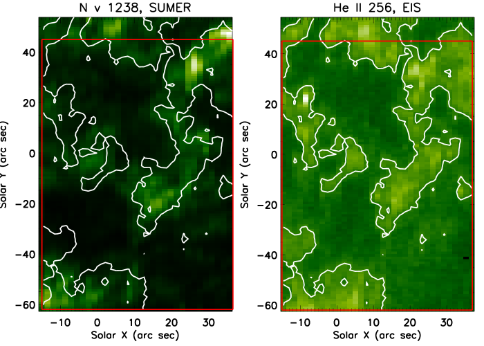
Figure 4: Radiance maps of the common area of study in N v $\lambda$1238 Å (SUMER, left) and He ii $\lambda$256 Å (EIS, right). Contours of He ii $\lambda$256 are plotted on both maps. The red boxes show the area in common to SUMER and the short and long wavelength ranges of EIS.

3 A method of measuring the Doppler velocity of EIS coronal lines

Above the limb we assume that spectral lines have, on average, no Doppler shift (motions out of the plane of sky cancel out on average). This is verified by plotting histograms of velocity (with respect to the average) and histograms of the distance in wavelength between a line and the reference Fe x $\lambda$184 line. These histograms are very narrow, nearly Gaussian, and have an FWHM of 3 km s^-1 to 4 km s^-1 (Figs. 5, 6).

From the above assumptions , the average of the off-limb line-distance histogram is then

$$\overline{\Delta\lambda_{off}}=\,\lambda_{0}-\lambda_{0}^{Ref},$$ (1)

where $\lambda_{0}^{Ref}$ and $\lambda_{0}$ are the rest wavelengths of the reference line and of the line whose shift we want to measure.

On the disk we measure the quantity $\Delta\lambda=\,\lambda-\lambda^{Ref}$ at each pixel or group of pixels (where $\lambda^{Ref}$ is the wavelength of the reference line). This can be written as

$$\Delta\lambda=\,\lambda_{0}+\delta\lambda\,-\,\lambda_{0}^{Ref}\,-\,\delta\lambda^{Ref}=\,\overline{\Delta\lambda_{off}}\,+\delta\lambda\,-\,\delta\lambda^{Ref},$$ (2)

where $\delta\lambda$ and $\delta\lambda^{Ref}$ are the line Doppler shifts. Considering that $v=c\frac{{\delta\lambda}}{{\lambda_{0}}}$, we have

$$\Delta\lambda=\,\overline{\Delta\lambda_{off}}\,+\frac{v}{c}\,\lambda_{0}\,-\frac{{v^{Ref}}}{c}\,\lambda_{0}^{Ref}.$$ (3)

If we call $\delta v=v-v^{Ref}$, the difference between the velocities measured in the two lines, then $\delta v$ becomes

$$\delta v\,=\,\,\frac{c}{{\lambda_{0}}}\left({\Delta\lambda\,-\,\overline{\Delta\lambda_{off}}\left({1+\frac{{v^{Ref}}}{c}}\right)}\right).$$ (4)

Considering now the average value of $v^{Ref}$, $\overline{v^{Ref}}$, we can write

$$\overline{\delta v}=\frac{c}{{\lambda_{0}}}\left({\overline{\Delta\lambda}-\overline{\Delta\lambda_{0ff}}\,\left({1+\frac{{\overline{v^{Ref}}}}{c}}\right)}\right).$$ (5)

We measure $\overline{\Delta\lambda}$ by taking the average of the distribution of wavelength differences between the two lines . Then, using equation (5) we calculate the relative velocity $\overline{\delta v}$ of hot coronal ions with respect to Fe x $\lambda$184 that we assume to have an average Doppler velocity $\overline{v^{Ref}}$ equal to the average Doppler velocity of Mg x $\lambda$625 ($-1.8\pm 0.6\leavevmode\nobreak\ \rm km\leavevmode\nobreak\ s^{-1}$).

Because of thermal variation along the 98.5 min Hinode orbit, there is a shift in the spectral line positions with time that needs to be corrected before using EIS data. Routines for correcting this variation are provided with the data reduction package and the correction has been applied to our data. However, we are not sure that the above correction (based on the data itself) is reliable down to the accuracy needed for the measurements discussed here ($\approx$ 2 km s^-1). A major advantage of the technique presented in this paper is that we do not rely on this correction because we are just measuring the spectral distances between spectral lines . We only need to make sure that all spectral lines move across the detectors in the same way, i.e., that there are no changes in the image scale with time. The top panel of Fig. 7 shows the dependence on time (and solar X) of line positions (averages along the slit, in wavelength units) for three lines (Fe x $\lambda$184, Fe x $\lambda$257, and Fe xii $\lambda$193) when no correction for temporal drifts is introduced. Offsets in wavelength (indicated in the figure) have been subtracted to make the comparison more evident. The behaviour of all the lines is very similar. The bottom panel of the figure shows line distances (differences in the values in the top panel) versus time and solar X. It can be seen that changes in line distance (wavelength differences) are very small ($\approx$1 mÅ, $\approx$ 1.5 km s^-1) and show no significant dependence with time. Hence our assumption is fulfilled.

To improve the signal-to-noise ratio, before fitting the line profiles we have binned the EIS on-disk spectra over three raster positions and over three pixels along the slit (3$\times$5 binning for the Fe xv $\lambda 284$, weak on the quiet Sun). A 2$\times$2 binning was used for the off-limb spectra.

Figure 5: The histograms of line position in wavelength for Fe xii $\lambda$193 line off-limb (dotted line) and at disk centre (solid line). The off-limb histogram is narrower than the on-disk one because net mass motions are essentially absent.

Figure 6: The histogram of distance in wavelength between Fe xii $\lambda$195 line and the reference line (Fe x $\lambda$184) off-limb. The histogram is nearly Gaussian and with a sigma of $\approx$ 1.3 km s^-1, that can be taken as an estimate of the instrument accuracy in measuring the distance in wavelength.

4 Results

Figure 7: Upper panel: line positions, in wavelength units, of the Fe xii $\lambda$193, Fe x $\lambda$257, and Fe x $\lambda$184 lines versus time (and solar X) at disk centre. The wavelength values indicated in the panel have been subtracted to ease comparison. Lower panel: wavelength difference between spectral lines for the data in the upper panel versus time (and solar X). It can be seen that changes in line distances (wavelength differences) are very small ($\approx$1 mÅ, $\approx$ 1.5 km s^-1) and show no dependence on time.

Using the technique discussed in Section 3 we have obtained the line of sight velocities from the Doppler shifts of many coronal lines formed at temperatures between 1 MK and 2 MK in the quiet Sun. These lines, their deduced relative (to Fe x $\lambda$184) Doppler shifts and the corresponding uncertainties are listed in Table 2. In this table, we report the values obtained in the four EIS raster scans together with the estimated errors. Errors are obtained by error propagation analysis of Eq. 5, where the error on $\overline{\Delta\lambda_{0ff}}$ is given by the width $\sigma$ of the off-limb line-distance distribution. On the other hand, the on-disk line distance distribution is also broadened by the different Doppler speeds characterising the two lines at different locations. For this reason the error for $\overline{\Delta\lambda}$ is assumed to be equal to that of $\overline{\Delta\lambda_{0ff}}$, leading to the same error for a given line in all the rasters. An independent estimate of these errors can be obtained by looking at the standard deviation of the measured values of $\overline{\delta v}$ obtained in the four rasters. From Table 2, values of 0.1 km s^-1 and 0.7 km s^-1 would be obtained for Fe xii $\lambda$195 and Fe xv $\lambda$284, respectively. These values are lower than our estimated errors and indicate the most likely we do not underestimate the errors provided in Table 2.

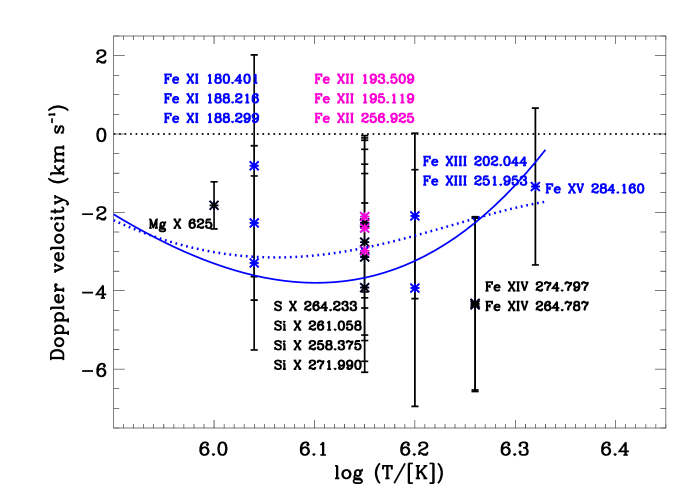
Figure 9: Magnification of the high-temperature part of Fig. 8 showing the results obtained in this work for coronal lines. Symbols and lines as in Fig. 8.

In the following, we take the average of rasters # 3 and # 4 as representative values of the average Doppler shift on the quiet Sun, the closest in time to the SUMER observations. By adding the value of average Doppler velocity of our reference line (Mg x $\lambda 625$) to these values ($\overline{v}=\overline{v^{Ref}}+\overline{\delta v}$), the absolute Doppler velocity of lines are calculated (see Table 3). The error reported in this table, $\delta(\overline{v})$, is obtained by summing in quadrature the errors on relative line Doppler shifts (reported in Table 2), and the error in measuring the average Doppler velocity of our reference line (Mg x $\lambda 625$). The values in Table 3) are plotted in Fig. 8 and as a blow-up for temperatures above 1 MK in Fig. 9.

Figure 8 displays the Doppler shift in the quiet Sun at disk centre of various TR and coronal ions in SUMER and EIS spectra. Positive values indicate red shifts (downflows), while negative values indicate blue shifts (upflows). Values obtained in this investigation (both SUMER and EIS) are marked by stars. In the figure the results of Teriaca et al. (1999a), Peter & Judge (1999), and the theoretical Doppler shifts of Hansteen et al. (2010) are also shown.

The solid and dashed lines respectively represent a by-eye fourth and sixth order polynomial representation of the combination of our present work for TR and coronal lines ($T\leq$ 2 MK) and those of Teriaca et al. (1999a). Thus, the $v$ $versus$ log($T/$[K]) behaviour can be parametrised by the coefficients that are listed in Table 4.

At temperatures higher than 1 MK our results show a modest but clear increase of the average blue shift with respect to the value measured around 1 MK ($-1.8$ km s^-1), reaching a maximum of about $-4.4$ km s^-1 at the Fe xiv formation temperature of 1.8 MK. At even higher temperatures, the average line shift appears to decrease again, reaching a value of $(-1.3\pm 2.6)$ km s^-1 obtained in Fe xv $\lambda$284 line at 2.1 MK.

To check if our results are dependent on the choice of our reference line (Fe x $\lambda$184), we have used another Fe x line ($\lambda$257) and calculated all Doppler velocities with respect to it. The Doppler velocities are found to agree within $1\leavevmode\nobreak\ \rm km\leavevmode\nobreak\ s^{-1}$ with those in Table 2.

It is clear that the absolute values of the velocities derived here depend on the value adopted for the reference line (in this case $-$1.8 km s^-1). To check the dependence of our results on the value of the velocity of our reference line (Fe x $\lambda$184, which we have supposed to have the same average Doppler velocity of Mg x $\lambda$625), we used Eq. 5 to calculate the absolute velocity for different values of the rest wavelength of the Mg x line (which ultimately determine the velocity in the reference line). The dependence of the Doppler shift on the Mg x rest wavelength and on the resulting Doppler velocity is shown in Fig. 10 for the Si x $\lambda$261, Fe xii $\lambda$195, Fe xiii $\lambda$251, Fe xiv $\lambda$264, and Fe xv $\lambda$284 lines. It should be noted that using the rest wavelength from Kelly (1987), would result in red shifts for most of the coronal lines studied here.

Table 2: Doppler velocity of ions with respect to Fe x $\lambda$184.

line	$\overline{\delta v}$				$\delta(\overline{\delta v})$
	[km s-1]				[km s-1]
	# 1	# 2	# 3	# 4
Fe x 257.262	0.86	0.28	0.52	1.44	2.30
Fe xi 180.401	0.96	1.14	0.76	1.22	2.77
Fe xi 188.216	0.15	-0.71	-0.25	-0.68	1.88
Fe xi 188.299	-1.35	-2.35	-1.41	-1.57	2.14
Si x 258.375	-0.41	-0.87	-1.57	-1.10	2.04
Si x 261.058	-0.96	-0.04	-1.19	-0.73	2.29
Si x 271.990	-1.51	-1.62	-2.06	-2.17	2.07
S x 264.233	0.21	-0.01	-0.47	-0.47	2.09
Fe xii 193.509	-0.64	-0.83	-0.16	-0.46	1.98
Fe xii 195.119	-0.52	-0.67	-0.52	-0.67	1.52
Fe xii 256.925	-0.54	-1.00	-1.70	-0.65	2.76
Fe xiii 202.044	-0.43	-0.73	-0.14	-0.43	2.02
Fe xiii 251.953	-1.54	-3.08	-2.84	-1.42	2.96
Fe xiv 264.787	-2.62	-2.96	-2.27	-2.84	2.13
Fe xiv 274.203	-2.47	-2.14	-3.45	-1.59	2.13
Fe xv 284.160	1.38	0.33	1.28	-0.31	2.56

• Columns 2 to 5 list the results for the four different rasters. The last column provides the error, which is equal for all rasters (see text).

Table 3: Absolute average Doppler velocity of ions (averaged over rasters #3 and #4).

line (log($T$/[K]))	$\overline{v}$ [km s-1]	$\delta(\overline{v})$ [km s-1] a
Fe x 184.536 (6.00)	-1.8 b	0.6 b
Fe x 257.262 (6.00)	-0.82	2.38
Fe xi 180.401 (6.04)	-0.81	2.83
Fe xi 188.216 (6.04)	-2.27	1.97
Fe xi 188.299 (6.04)	-3.29	2.22
Si x 258.375 (6.15)	-3.14	2.13
Si x 261.058 (6.15)	-2.76	2.37
Si x 271.990 (6.15)	-3.92	2.16
S x 264.233 (6.15)	-2.27	2.17
Fe xii 193.509 (6.15)	-2.11	2.07
Fe xii 195.119 (6.15)	-2.40	1.63
Fe xii 256.925 (6.15)	-2.98	2.82
Fe xiii 202.044 (6.20)	-2.09	2.11
Fe xiii 251.953 (6.20)	-3.93	3.02
Fe xiv 264.787 (6.26)	-4.36	2.21
Fe xiv 274.203 (6.26)	-4.32	2.21
Fe xv 284.160 (6.32)	-1.34	2.63

• ^a The last column provides the error on the absolute average Doppler velocities (see text).

• ^b Absolute velocity and error assumed equal to that of Mg x.

Table 4: Coefficients of the fourth and sixth order polynomial representations of the average Doppler velocity versus temperature behaviour of the quiet Sun.

coefficient	$4^{th}$ order	$6^{th}$ order
a0	7874.8	-185202.25
a1	-6427.5	223219.47
a2	1943.26	-111257.36
a3	-257.766	29345.005
a4	12.6596	-4319.1993
a5		336.35535
a6		-10.827987

• All decimals shown here are significant.

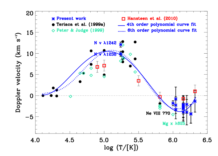
Figure 8: Average Doppler shift in the quiet Sun at disk centre of various TR and coronal ions measured from SUMER and EIS spectra. Positive values indicate red shifts (downflows) while negative values indicate blue shifts (upflows). Solid and dashed lines respectively represent fourth and and sixth order polynomial curves by-eye fitted to the combination of the measurements obtained in this work and those of Teriaca et al. (1999a).

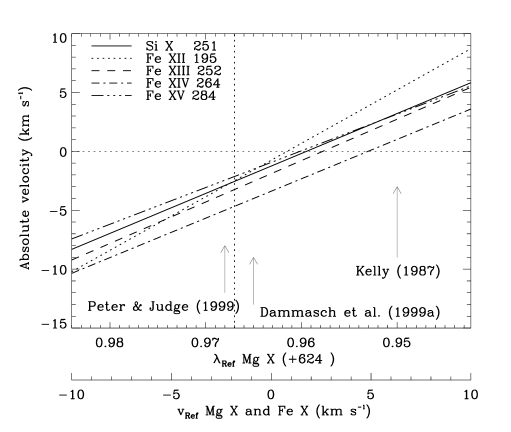
Figure 10: Variation in the absolute Doppler velocity of hot coronal ions as a function of the rest wavelength of the Mg x line and, consequently, of the Doppler velocity from the Fe x $\lambda$184 reference line. The vertical dotted line corresponds to the adopted rest wavelength of 624.967 Å.

5 Summary and conclusions

In the present study we measured the Doppler shift of TR and coronal lines on the quiet Sun (see Tables 1 & 3). We measured the absolute average velocity of Mg x $\lambda$625, N v $\lambda$1238, and N v $\lambda$1242 lines using SUMER data obtaining a blue shifted Doppler velocity of ($-1.8\pm 0.6$) km s^-1 for Mg x $\lambda$625 and red shifts (downward motions) of ($9.9\pm 0.6$) and ($12.1\pm 0.6$) for the N v $\lambda$1238 and $\lambda$1242 lines. Our results for TR lines agree with previous studies done with SUMER (Brekke et al. 1997; Chae et al. 1998; Peter & Judge 1999; Teriaca et al. 1999a). Our result for the Mg x line is also consistent with the literature, once the differences on the adopted rest wavelength are accounted for (see Section 2.1). Of course, our value for the average shift in the Mg x line depends on the adopted rest wavelength of 624.967 Å  (Dammasch et al. 1999a; Peter & Judge 1999, average between the values of). Since the velocities obtained from the EIS lines also depend on the absolute velocity of the Mg x ions, the precise determination of the rest wavelength of Mg x is paramount. The accurate, independent, and highly consistent measurements of Dammasch et al. (1999a) and Peter & Judge (1999) are the best available so far. In any case, Fig. 10 allows assessing the effect of a different rest wavelength for the Mg x $\lambda 625$ line on the resulting Doppler shifts.

By using cospatial and nearly cotemporal SUMER & EIS data we, for the first time, measured the average Doppler shift of several coronal lines with formation temperatures above 1 MK in the quiet Sun near disk centre. We obtained negative Doppler shifts (upward motions) between -2 to -4 km s^-1 at temperatures between 1 and 1.8 MK. At the highest temperature we can investigate, $T=2.1$ MK (Fe xv $\lambda 284$), we find indications of a reduction of the observed blue shift down to 1.3 km s^-1, a value that is compatible with no line shift, but also with a blue shift of up to 4 km s^-1.

As discussed in the Introduction, 1-D models assuming energy release in magnetic loops had successfully managed to reproduce the observer red shift at TR temperatures and blue shifts at coronal temperatures (e.g., Teriaca et al. 1999b; Spadaro et al. 2006). However, these models do not explicitly consider the heating mechanism.

More recently, comprehensive 3-D models of the solar atmosphere have been developed. Models assuming that coronal heating is caused by Joule dissipation of currents produced by stressing and braiding of the magnetic field produce red shifts at all temperatures (Peter et al. 2004, 2006), which is contrary to the present results and those of (Peter & Judge 1999) and (Teriaca et al. 1999a).

The addition to the model of episodic injections of emerging magnetic flux that reconnects with the existing field, produces rapid, episodic heating of the upper chromospheric plasma to coronal temperatures (Hansteen et al. 2010). Doppler shifts are computed by these authors for a model with an unsigned magnetic field of $\mid B_{z}\mid\approx$ 75 G, which is compatible with the quiet Sun (Trujillo Bueno et al. 2004; Domínguez Cerdeña et al. 2006; Danilovic et al. 2010). The resulting Doppler shifts are roughly consistent with those reported here at all temperatures up to the Fe xiv formation temperature (log($T$/[K])=6.26) (see Fig. 8). Above this value, the line shifts predicted by the model return to zero and become slightly red shifted at the Fe xv formation temperature (log($T$/[K])=6.32).

Our Fe xv observations, instead, yield a blue shifted value. However, the error bar is large enough that no firm conclusion can be drawn. A real discrepancy at this temperature between the observations and the model may possibly be due to boundary effects in the adopted computing box or, more simply, to the fact that the turning point to zero or red shifted values occurs in reality at temperatures even higher than those measurable in this study. However, it may also be possible that important ingredients are still missing in the theoretical/numerical description.

Hansteen et al. (2010) suggest that the high speed flows generated by the localised heating events may be related to the high speed upflows that have been deduced from significant blueward asymmetries in Hinode/EIS observations of many TR and coronal lines (Hara et al. 2008; De Pontieu et al. 2009; McIntosh & De Pontieu 2009b, a) that have been linked to spicules (De Pontieu et al. 2011). Thus, a more accurate introduction of the effect of spicules into the model may be necessary.

The model also foresees a smaller amount of Doppler shifts at both TR (lower red shifts) and coronal temperatures (lower blue shifts). However, this is not surprising (as the model does not specifically attempt to reproduce the solar region studied here), and the model is most likely compatible with our measurement. Since the model does not consider open field lines, this would indicate that the observed line shifts are simply a by-product of the heating of, and related mass supply to, closed loops. This would be consistent with the finding that the plasma outflows seen on the quiet Sun, such as the Ne viii blue shift, are largely associated with closed loops (Tian et al. 2008).

However, it cannot also be excluded that hot open funnels significantly contribute to the blue shifted emission observed between 1 and 2 MK. Only a detailed analysis of spatially resolved flows compared to field extrapolations (similar to what was done for the Ne viii line at lower temperatures by Tian et al. 2008) would shed some light on the question. Given that these hotter lines are weak on the quiet Sun, this analysis is very difficult and will require a VUV spectrometer with much higher throughput than currently available, such as the spectrometer proposed for the Japanese Solar C mission (Teriaca et al. 2011).