Abstract

This article describes posterior maximization for topic models, identifying computational and conceptual gains from inference under a non-standard parametrization. We then show that fitted parameters can be used as the basis for a novel approach to marginal likelihood estimation, via block-diagonal approximation to the information matrix, that facilitates choosing the number of latent topics. This likelihood-based model selection is complemented with a goodness-of-fit analysis built around estimated residual dispersion. Examples are provided to illustrate model selection as well as to compare our estimation against standard alternative techniques.

1 Introduction

A topic model represents multivariate count data as multinomial observations parameterized by a weighted sum of latent topics. With each observation $\mathbf{x}_{i}\in\{\mathbf{x}_{1}\ldots\mathbf{x}_{n}\}$ a vector of counts in $p$ categories, given total count $m_{i}=\sum_{j=1}^{p}x_{ij}$, the $K$-topic model has

$$\mathbf{x}_{i}\sim\mathrm{MN}(\omega_{i1}\boldsymbol{\theta}_{1}+\ldots+\omega_{iK}\boldsymbol{\theta}_{K},m_{i})$$ (1)

where topics $\boldsymbol{\theta}_{k}=[\theta_{k1}\cdots\theta_{kp}]^{\prime}$ and weights $\boldsymbol{\omega}_{i}$ are probability vectors. The topic label is due to application of the model in (1) to the field of text analysis. In this context, each $\mathbf{x}_{i}$ is a vector of counts for terms (words or phrases) in a document with total term-count $m_{i}$, and each topic $\boldsymbol{\theta}_{k}$ is a vector of probabilities over words. Documents are thus characterized through a mixed-membership weighting of topic factors and, with $K$ far smaller than $p$, each $\boldsymbol{\omega}_{i}$ is a reduced dimension summary for $\mathbf{x}_{i}$.

Section 2 surveys the wide use of topic models and emphasizes some aspects of current technology that show room for improvement. Section 2.1 describes how common large-data estimation for topics is based on maximization of an approximation to the marginal likelihood, $\mathrm{p}(\mathbf{X}|\boldsymbol{\Theta})$. This involves very high-dimensional latent variable augmentation, which complicates and raises the cost of computation, and independence assumptions in approximation that can potentially bias estimation. Moreover, Section 2.2 reviews the very limited literature on topic selection, arguing the need of new methodology for choosing $K$.

The two major objectives of this article are thus to facilitate an efficient alternative for estimation of topic models, and to provide a default method for model selection. In the first case, Section 3 develops a framework for joint posterior maximization over both topics and weights: given the parameterization described in 3.1, we outline a block-relaxation algorithm in 3.2 that augments expectation-maximization with quadratic programming for each $\boldsymbol{\omega}_{i}$. Section 4 then presents two possible metrics for model choice: 4.1 describes marginal data likelihood estimation through block-diagonal approximation to the information matrix, while 4.2 proposes estimation for residual dispersion. We provide simulation and data examples in Section 5 to support and illustrate our methods, and close with a short discussion in Section 6.

2 Background

The original text-motivated topic model is due to Hofmann (1999), who describes its mixed-membership likelihood as a probability model for the latent semantic indexing of Deerwester et al. (1990). Blei et al. (2003) then introduce the contemporary Bayesian formulation of topic models as latent Dirichlet allocation (LDA) by adding conditionally conjugate Dirichlet priors for topics and weights. This basic model has proven hugely popular, and extensions include hierarchical formulations to account for an unknown number of topics (Teh et al., 2006, using Dirichlet processes), topics that change in time (Blei and Lafferty, 2006) or whose expression is correlated (Blei and Lafferty, 2007), and topics driven by sentiment (Blei and McAuliffe, 2010). Equivalent likelihood models, under both classical and Bayesian formulation, have also been independently developed in genetics for analysis of population admixtures (e.g., Pritchard et al., 2000).

2.1 Estimation Techniques

This article, as in most text-mining applications, focuses on a Bayesian specification of the model in (1) with independent priors for each $\boldsymbol{\theta}_{k}$ and $\boldsymbol{\omega}_{i}$, yielding a posterior distribution proportional to

$$\mathrm{p}(\boldsymbol{\Theta},\boldsymbol{\Omega},\mathbf{X})=\prod_{i=1}^{n}\mathrm{MN}(\mathbf{x}_{i};\boldsymbol{\Theta}\boldsymbol{\omega}_{i},m_{i})\mathrm{p}(\boldsymbol{\omega}_{i})\prod_{k=1}^{K}\mathrm{p}(\boldsymbol{\theta}_{k}).$$ (2)

Posterior approximations rely on augmentation with topic membership for individual terms: assume term $l$ from document $i$ has been drawn with probability given by topic $\boldsymbol{\theta}_{z_{il}}$, where membership $z_{il}$ is sampled from the $K$ available according to $\boldsymbol{\omega}_{i}$, and write $\mathbf{z}_{i}$ as the $m_{i}$-length indicator vector for each document $i$ and $\mathbf{Z}=\{\mathbf{z}_{1},\ldots,\mathbf{z}_{n}\}$ as the full latent parameter matrix.

Gibbs sampling for this specification is described in the original genetic admixture paper by Pritchard et al. (2000) and by some in machine learning (e.g., Griffiths and Styvers, 2004). Many software packages adapt Gibbs to large-data settings by using a single posterior draw of $\mathbf{Z}$ for parameter estimation. This only requires running the Markov chain until it has reached its stationary distribution, instead of the full convergence assumed in mean estimation, but the estimates are not optimal or consistent in any rigorous sense.

It is more common in practice to see variational posterior approximations (Wainwright and Jordan, 2008), wherein some tractable distribution is fit to minimize its distance from the unknown true posterior. For example, consider the conditional posterior $\mathrm{p}(\boldsymbol{\Omega},\mathbf{Z}\mid\boldsymbol{\Theta},\mathbf{X})$ and variational distribution $\mathrm{q}(\boldsymbol{\Omega},\mathbf{Z})=\prod_{i=1}^{n}\left[\mathrm{Dir}(\boldsymbol{\omega_{i}};\mathbf{s}_{i})\prod_{l=1}^{m_{i}}\mathrm{MN}(z_{il};\mathbf{r}_{il})\right]$. Kullback-Leibler divergence between these densities is

$$- \int\log\frac{\mathrm{p}(\boldsymbol{\Omega},\mathbf{Z}~{}|~{}\boldsymbol{\Theta},\mathbf{X})}{\mathrm{q}(\boldsymbol{\Omega},\mathbf{Z})}d\mathrm{Q}(\boldsymbol{\Omega},\mathbf{Z})$$ (3)

$$~{}~{}=\log\mathrm{p}(\mathbf{X}\mid\boldsymbol{\Theta})$$

$$~{}~{}~{}~{}~{}~{}~{}-\left\{\mathds{E}_{q}\left[\log\mathrm{p}(\boldsymbol{\Omega},\mathbf{Z},\mathbf{X}\mid\boldsymbol{\Theta})\right]-\mathds{E}_{q}\left[\log\mathrm{q}(\boldsymbol{\Omega},\mathbf{Z})\right]\right\},$$

which is minimized by maximizing the lower bound on marginal likelihood for $\boldsymbol{\Theta}$, $\mathds{E}_{q}\left[\log\mathrm{p}(\boldsymbol{\Omega},\mathbf{Z},\mathbf{X}\mid\boldsymbol{\Theta})\right]-\mathds{E}_{q}\left[\log\mathrm{q}(\boldsymbol{\Omega},\mathbf{Z})\right]$, as a function of $\mathrm{q}$’s tuning parameters. Since $\boldsymbol{\omega}_{i}\perp\!\!\!\perp\boldsymbol{\omega}_{l}$ for $i\neq l$ conditional on $\boldsymbol{\Theta}$, $\mathrm{q}$’s main relaxation is assumed independence of $\mathbf{Z}$.

The objective in (3) is proposed in the original LDA paper by Blei et al. (2003). The most common approach to estimation (e.g., Blei and Lafferty, 2007; Grimmer, 2010, and examples in Blei et al. 2003) is then to maximize $\mathds{E}_{q}\left[\log\mathrm{p}(\boldsymbol{\Omega},\mathbf{Z},\mathbf{X}\mid\boldsymbol{\Theta})\right]$ given $\mathrm{q}(\boldsymbol{\Omega},\mathbf{Z})\approx\mathrm{p}(\boldsymbol{\Omega},\mathbf{Z}~{}|~{}\boldsymbol{\Theta},\mathbf{X})$. This mean-field estimation can be motivated as fitting $\boldsymbol{\widehat{\Theta}}$ to maximize the implied lower bound on $\mathrm{p}(\mathbf{X}\mid\boldsymbol{\Theta})$ from (3), and thus provides approximate marginal maximum likelihood estimation. The procedure is customarily identified with its implementation as a variational EM (VEM) algorithm, which iteratively alternates between conditional minimization of (3) and maximization of the bound on $\mathrm{p}(\mathbf{X}~{}|~{}\boldsymbol{\Theta})$.

A second strategy, full variational Bayes, constructs a joint distribution through multiplication of $\mathrm{q}(\boldsymbol{\Omega},\mathbf{Z})$ by $\mathrm{q}(\boldsymbol{\Theta})=\prod_{k=1}^{K}\mathrm{Dir}(\boldsymbol{\theta}_{k}\mid\mathbf{u}_{k})$ and minimizes KL divergence against the full posterior. However, since cross-topic posterior correlation $\mathrm{cor}(\theta_{kj},\theta_{hj})$ does not disappear asymptotically, the independence assumption of $\mathrm{q}(\boldsymbol{\Theta})$ risks inconsistency for $\boldsymbol{\widehat{\Theta}}$ and unstable finite sample results (e.g., Teh et al., 2006).

Our proposed approach is distinct from the above in seeking joint MAP solution for both $\boldsymbol{\Theta}$ and $\boldsymbol{\Omega}$ (i.e., that which maximizes (2)), thus altogether avoiding posterior approximation. The estimation methodology of Section 3 is more closely connected to maximum likelihood estimation (MLE) techniques from the non-Bayesian literature on topic models: the EM algorithm, as used extensively for genetics admixture estimation (e.g., Tang et al., 2006) and in Hoffman’s 1999 text-analysis work, and quadratic programming as applied by Alexander et al. (2009) in a fast block-relaxation routine. We borrow from both strategies.

Comparison between MAP and VEM estimation is simple: the former finds jointly optimal profile estimates for $\boldsymbol{\Theta}$ and $\boldsymbol{\Omega}$, while the latter yields inference for $\boldsymbol{\Theta}$ that is approximately integrated over uncertainty about $\boldsymbol{\Omega}$ and $\mathbf{Z}$. There are clear advantages to integrating over nuisance parameters (e.g., Berger et al., 1999), but marginalization comes at the expense of introducing a very high dimensional latent parameter ($\mathbf{Z}$) and its posterior approximation. This leads to algorithms that are not scaleable in document length, potentially with higher variance estimation or unknown bias. We will find that, given care in parameterization, exact joint parameter estimation can be superior to approximate marginal inference.

2.2 Choosing the Number of Topics

To learn the number of topics from data, the literature makes use of three general tools: cross-validation, nonparametric mixture priors, and marginal likelihood. See Airoldi et al. (2010) for a short survey and comparison. Cross-validation (CV) is by far the most common choice (e.g. Grimmer, 2010; Grün and Hornik, 2011). Unfortunately, due to the repeated model-fitting required for out-of-sample prediction, CV is not a large-scale method. It also lacks easy interpretability in terms of statistical evidence, or even in terms of sample error (Hastie et al., 2009, 7.12). For a model-based alternative, Teh et al. (2006) write LDA as a Hierarchical Dirichlet process with each document’s weighting over topics a probability vector of infinite length. This removes the need to choose $K$, but estimation can be sensitive to the level of finite truncation for these prior processes and will always require inference about high-dimensional term-topic memberships. Finally, the standard Bayesian solution is to maximize the marginal model posterior. However, marginal likelihood estimation in topic models has thus far been limited to very rough approximation, such as the average of MCMC draws in (Griffiths and Styvers, 2004).

3 Parameter Estimation

Prior choice for latent topics can be contentious (Wallach et al., 2009) and concrete guidance is lacking in the literature. We consider simple independent priors, but estimation updates based on conditional independence make it straightforward to adapt for more complex schemes. Our default specification follows from a general preference for simplicity. Given $K$ topics,

$$\boldsymbol{\omega}_{i} \stackrel{{\scriptstyle iid}}{{\sim}}\mathrm{Dir}(1/K),~{}i=1\ldots n,$$ (4)

$$\boldsymbol{\theta}_{k} \stackrel{{\scriptstyle iid}}{{\sim}}\mathrm{Dir}(\alpha_{k1},\ldots,\alpha_{kp}),~{}k=1\ldots K.$$

The single Dirichlet concentration parameter of $1/K$ for each $\boldsymbol{\omega}$ encourages sparsity in document weights by placing prior density at the edges of the parameter space. This specification is also appropriate for model selection: weight of prior evidence is constant for all values of $K$, and as $K$ moves to infinity $\mathrm{Dir}(1/K)$ approaches the Dirichlet process (Neal, 2000). Topic priors are left generic in (4) to encourage flexibility but we default to the low concentration $\alpha_{kj}=1/(Kp)$.

3.1 Natural Exponential Family Parameterization

To improve estimation stability and efficiency, we propose to solve for MAP estimates of $\boldsymbol{\Omega}$ and $\boldsymbol{\Theta}$ not in the original simplex space, but rather after transform into their natural exponential family (NEF) parameterization. For example, in the case of $\boldsymbol{\Omega}$ we seek the MAP estimate for $\boldsymbol{\Phi}=\{\boldsymbol{\varphi}_{1},\ldots,\boldsymbol{\varphi}_{n}\}$, where for a given $\boldsymbol{\omega}$,

$$\omega_{k}=\frac{\exp[{\varphi_{k-1}}]}{\sum_{h=0}^{K-1}\exp[{\varphi_{h}}]},~{}~{}\text{with~{}the~{}fixed~{}element}~{}~{}\varphi_{0}=0.$$ (5)

Hence, ignoring $\varphi_{i0}$ in estimation, each $\boldsymbol{\varphi}_{i}$ is an unrestricted vector of length $K-1$. Since $\partial\omega_{k}/\partial\varphi_{h}=\mathds{1}_{k=h}\omega_{k}-\omega_{k}\omega_{h}$, the Jacobian for this transformation is $\mathrm{Diag}[\boldsymbol{\omega}]-\boldsymbol{\omega}\boldsymbol{\omega}^{\prime}$ and has determinant $|\mathrm{Diag}[\boldsymbol{\omega}]|(1-\boldsymbol{\omega}^{\prime}\mathrm{Diag}[\boldsymbol{\omega}]\boldsymbol{\omega})=\prod_{k=1}^{K-1}\omega_{k}(1-\sum_{h=1}^{K-1}\omega_{h})$. Hence, viewing each $\boldsymbol{\omega}_{i}$ as a function of $\boldsymbol{\varphi}_{i}$, the conditional posterior for each individual document given $\boldsymbol{\Theta}$ becomes

$$\mathrm{p} (\boldsymbol{\omega}_{i}(\boldsymbol{\varphi}_{i})\mid\mathbf{x}_{i})$$ (6)

$$\propto\mathrm{MN}(\mathbf{x}_{i};\boldsymbol{\Theta}\boldsymbol{\omega}_{i},m_{i})\prod_{k=1}^{K-1}\omega_{k}^{1/K}\left(1-\sum_{h=1}^{K-1}\omega_{h}\right)^{1/K},$$

and the NEF conditional MAP is equivalent to solution for $\boldsymbol{\omega}$ under a $\mathrm{Dir}(1/K+1)$ prior. Similarly, our estimate for each $\boldsymbol{\theta}_{k}$ corresponds to the simplex MAP under a $\mathrm{Dir}(\boldsymbol{\alpha}_{k}+1)$ prior.

The NEF transformation leads to conditional posterior functions that are everywhere concave, thus guaranteeing a single conditional MAP solution for each $\boldsymbol{\omega}_{i}$ given $\boldsymbol{\Theta}$. This introduces stability into our block relaxation algorithm of 3.2: without moving to NEF space, the prior in (4) with $1/K<1$ could lead to ill-defined maximization problems at each iteration. Conditional posterior concavity also implies non-boundary estimates for $\boldsymbol{\Omega}$, despite our use of sparsity encouraging priors, that facilitate Laplace approximation in Section 4.1.

3.2 Joint Posterior Maximization

We now detail joint MAP estimation for $\boldsymbol{\Omega}$ and $\boldsymbol{\Theta}$ under NEF parameterization. First, note that it is straightforward to build an EM algorithm around missing data arguments. In the MLE literature (e.g., Hofmann, 1999; Tang et al., 2006) authors use the full set of latent phrase-memberships ($\mathbf{Z}$) to obtain a mixture model specification. However, a lower dimensional strategy is based on only latent topic totals, such that each document $i=1\ldots n$ is expanded

$$\mathbf{X}_{i}\sim\mathrm{MN}_{p}(\boldsymbol{\theta}_{1},t_{i1})+\cdots+\mathrm{MN}_{p}(\boldsymbol{\theta}_{K},t_{iK}),$$ (7)

where $\mathbf{T}_{i}\sim\mathrm{MN}_{K}(\boldsymbol{\omega}_{i},m_{i})$, with $\mathbf{T}_{1}\ldots\mathbf{T}_{n}$ treated as missing-data. Given current estimates $\boldsymbol{\widehat{\Theta}}$ and $\boldsymbol{\widehat{\Omega}}$, standard EM calculations lead to approximate likelihood bounds of $\mathrm{MN}\left(\mathbf{\hat{X}}_{k};\boldsymbol{\theta}_{k},\hat{t}_{k}\right)$, with

$$\hat{x}_{kj}=\sum_{i=1}^{n}x_{ij}\frac{\hat{\theta}_{kj}\hat{\omega}_{ik}}{\sum_{h=1}^{K}\hat{\theta}_{hj}\hat{\omega}_{ih}},~{}~{}\hat{t}_{k}=\sum_{j=1}^{p}\hat{x}_{kj},~{}~{}k=1\ldots K.$$ (8)

Updates for NEF topic MAPs under our model are then $\theta_{kj}=(\hat{x}_{kj}+\alpha_{kj})/[\hat{t}_{k}+\sum_{j=1}^{p}\alpha_{kj}]$.

EM algorithms – even the low dimensional version in (8) – are slow to converge under large-$p$ vocabularies. We advocate finding exact solutions for $\boldsymbol{\Omega}\mid\boldsymbol{\Theta}$ at each iteration, as this can speed-up convergence by several orders of magnitude. Factorization of the conditional posterior makes for fast parallel updates that, similar to the algorithm of Alexander et al. (2009), solve independently for each $\boldsymbol{\omega}_{i}$ through sequential quadratic programming. We also add first-order quasi-Newton acceleration for full-set updates (Lange, 2010).

Suppressing $i$, each document’s conditional log posterior is proportional to

$$l(\boldsymbol{\omega})=\sum_{j=1}^{p}x_{j}\log\left(\omega_{1}\theta_{1j}+\ldots+\omega_{K}\theta_{Kj}\right)+\sum_{k=1}^{K}\frac{\log(\omega_{k})}{K},$$ (9)

subject to the constraints $\boldsymbol{1}^{\prime}\boldsymbol{\omega}=1$ and $\omega_{k}>0$ for $k=1\ldots K$. Gradient and curvature are then

$$g_{k} =\sum_{j=1}^{p}\frac{x_{j}\theta_{kj}}{\boldsymbol{\theta}^{\prime}_{j}\boldsymbol{\omega}}+\frac{1}{K\omega_{k}}$$ (10)

$$h_{kh} =-\sum_{j=1}^{p}\frac{x_{j}\theta_{kj}\theta_{hj}}{(\boldsymbol{\theta}^{\prime}_{j}\boldsymbol{\omega})^{2}}-\mathds{1}_{[k=h]}\frac{1}{K\omega_{k}^{2}}$$

and Taylor approximation around current estimate $\boldsymbol{\hat{\omega}}$ yields the linear system

$$\left[\begin{array}[]{cc}-\mathbf{h}&\boldsymbol{1}\\ \boldsymbol{1}^{\prime}&0\end{array}\right]\left[\begin{array}[]{c}\boldsymbol{\Delta}\\ \lambda\end{array}\right]=\left[\begin{array}[]{c}\mathbf{g}\\ 0\end{array}\right]$$ (11)

where $\Delta_{k}=(\omega_{k}-\hat{\omega}_{k})$ and $\lambda$ is the Lagrange multiplier for the equality constraint. This provides the basis for an active set strategy (Luenberger and Ye, 2008, 12.3): given $\boldsymbol{\Delta}$ solving (11), take maximum $\delta\in(0,1)$ such that $\delta\Delta_{k}<-\hat{\omega}_{k}~{}\forall k$, and set $\boldsymbol{\omega}=\boldsymbol{\hat{\omega}}+\delta\boldsymbol{\Delta}$. If $\delta<1$ and $\omega_{k}$ lies at boundary of the feasible region (i.e., some tolerance from zero), we activate that constraint by removing $\Delta_{k}$ and solving the simpler system.

Note from (10) that our log posterior in (9) is concave, thus guaranteeing a unique solution at every iteration. This would not be true but for the fact that we are actually solving for conditional MAP $\boldsymbol{\varphi}$, rather than $\boldsymbol{\omega}$. While the full joint posterior for transformed $\boldsymbol{\Theta}$ and $\boldsymbol{\Omega}$ obviously remains multi-modal (most authors use multiple starts to avoid minor modes; we initialize with a build from $2,\ldots,K$ topics by repeatedly fitting an extra topic to the residuals), the NEF parameterization introduces helpful stability at each iteration.

4 Model Selection

In this section, we propose two techniques for inferring the number of topics. The first approach, in 4.1, is an efficient approximation for the fully Bayesian procedure of marginal posterior maximization. The second approach, in 4.2, consists of a basic analysis of residuals. Both methods require almost no computation beyond the parameter estimation of Section 3.

4.1 Marginal Likelihood Maximization

Bayesian model selection is founded on the marginal data likelihood (see Kass and Raftery, 1995), and in the absence of a null hypothesis scenario or an informative model prior, we wish to find $K$ to maximize $\mathrm{p}(\mathbf{X}\mid K)=\int\mathrm{p}(\boldsymbol{\Theta},\boldsymbol{\Omega},\mathbf{X}\mid K)d\mathrm{P}(\boldsymbol{\Theta},\boldsymbol{\Omega})$. It should be possible to find a maximizing argument simply by evaluating $\mathrm{p}(\mathbf{X}\mid K)$ over possible values. However, as is often the case, the integral is intractable for topic models and must be approximated.

One powerful approach is Laplace’s method (Tierney and Kadane, 1986) wherein, assuming that the posterior is highly peaked around its mode, the joint parameter-data likelihood is replaced with a close-matching and easily integrated Gaussian density. In particular, quadratic expansion of $\log[\mathrm{p}(\mathbf{X},\boldsymbol{\Phi},\boldsymbol{\Theta})]$ is exponentiated to yield the approximate posterior, $\mathrm{N}([\boldsymbol{\Phi},\boldsymbol{\Theta}];[\boldsymbol{\hat{\Phi}},\boldsymbol{\hat{\Theta}}],\mathbf{H})$, where $[\boldsymbol{\hat{\Phi}},\boldsymbol{\hat{\Theta}}]$ is the joint MAP and $\mathbf{H}$ is the log posterior Hessian evaluated at this point. After scaling by $K!$ to account for label switching, these approximations have proven effective for general mixtures (e.g. Roeder and Wasserman, 1997).

As one of many advantages of NEF parameterization (Mackay, 1998), we avoid boundary solutions where Laplace’s approximation would be invalid. The integral target is also lower dimensional, although we leave $\boldsymbol{\Theta}$ in simplex representation due to a denser and harder to approximate Hessian after NEF transform. Hence,

$$\mathrm{p}(\mathbf{X}\mid K)\approx\mathrm{p}\left(\mathbf{X},\boldsymbol{\hat{\Theta}},\boldsymbol{\hat{\Omega}}\right)|-\mathbf{H}|^{-\frac{1}{2}}(2\pi)^{\frac{d}{2}}K!$$ (12)

where $d=Kp+(K-1)n$ is model dimension and $\mathrm{p}(\mathbf{X},\boldsymbol{\hat{\Theta}},\boldsymbol{\hat{\Omega}})=\prod_{i=1}^{n}\mathrm{MN}(\mathbf{x}_{i};\boldsymbol{\hat{\Theta}}\boldsymbol{\hat{\omega}}_{i},m_{i})\mathrm{Dir}(\boldsymbol{\hat{\omega}}_{i};1/K\!+\!1)$ $\prod_{k=1}^{K}\mathrm{Dir}(\boldsymbol{\hat{\theta}}_{k};\boldsymbol{\alpha}_{k}+1)$. In practice, to account for weight sparsity, we replace $d$ with $Kp+d_{\boldsymbol{\Omega}}$ where $d_{\boldsymbol{\Omega}}$ is the number of $\omega_{ik}$ greater than $1/1000$.

After parameter estimation, the only additional computational burden of (12) is finding the determinant of negative $\mathbf{H}$. Unfortunately, given the large $p$ and $n$ of text analysis, this burden will usually be significant and unaffordable. Determinant approximation for marginal likelihoods is not uncommon; for example, Bayes information criterion (BIC) can be motivated by setting $|-\mathbf{H}|\approx n^{d}|\mathbf{i}|$, with $\mathbf{i}$ the information matrix for a single observation. Although BIC convergence results do not apply under $d$ that depends on $n$, efficient computation is possible through a more subtle approximation based on block-diagonal factorization.

Writing $L=\log\left[\mathrm{p}(\mathbf{X},\boldsymbol{\Theta},\boldsymbol{\Omega})\right]$, diagonal blocks of $\mathbf{H}$ are

$$\mathbf{H}_{\boldsymbol{\Theta}}=\frac{\partial^{2}L}{\partial\boldsymbol{\Theta}^{2}}=\mathrm{Diag}\left[\displaystyle\frac{\partial^{2}L}{\partial\boldsymbol{\theta}_{\bullet 1}^{2}}\cdots\displaystyle\frac{\partial^{2}L}{\partial\boldsymbol{\theta}_{\bullet p}^{2}}\right]$$

$$\mathbf{H}_{\boldsymbol{\Phi}}=\frac{\partial^{2}L}{\partial\boldsymbol{\Phi}^{2}}=\mathrm{Diag}\left[\displaystyle\frac{\partial^{2}L}{\partial\boldsymbol{\varphi}_{1}^{2}}\cdots\frac{\partial^{2}L}{\partial\boldsymbol{\varphi}_{n}^{2}}\right]$$ (13)

where $\boldsymbol{\theta}_{\bullet j}=[\theta_{1j}\cdots\theta_{Kj}]$ is the $j^{th}$ row of $\boldsymbol{\Theta}$. Here,

$$\frac{\partial^{2}L}{\partial\theta_{kj}\partial\theta_{hj}}=\sum_{i=1}^{n}x_{ij}\frac{\omega_{ik}\omega_{ih}}{q_{ij}^{2}}+\mathds{1}_{k=h}\frac{\alpha_{jk}}{\theta_{kj}^{2}},$$

while for each individual document’s $\boldsymbol{\varphi}_{i}$,

$$\frac{\partial^{2}L}{\partial\varphi_{ik}\partial\varphi_{ih}}=\mathds{1}_{[k=h]}\omega_{k}-\omega_{ik}\omega_{ih}$$

$$-\sum_{j=1}^{p}x_{ij}\left[\mathds{1}_{[k=h]}\omega_{ik}\frac{\theta_{kj}-q_{ij}}{q_{ij}}+\omega_{ik}\omega_{ih}\left(1-\frac{\theta_{kj}\theta_{hj}}{q_{ij}^{2}}\right)\right]$$

with $q_{ij}=\sum_{k=1}^{K}\omega_{ik}\theta_{kj}$. Finally, the sparse off-diagonal blocks of $\mathbf{H}$ have elements

$$\frac{\partial^{2}L}{\partial\theta_{jk}\partial\varphi_{ih}}=-x_{ij}\left[\frac{\omega_{ik}\omega_{ih}}{q_{ij}^{2}}\theta_{hj}-\frac{\omega_{ih}}{q_{ij}}\mathds{1}_{[k=h]}\right]$$

wherever $x_{ij}\neq 0$, and zero otherwise. Ignoring these cross curvature terms, an approximate determinant is available as the product of determinants for each diagonal block in (4.1). That is, our marginal likelihood estimate is as in equation (12), but with replacement

$$\left|-\mathbf{H}\right|\approx\left|\begin{array}[]{cc}-\mathbf{H}_{\mathbf{\Theta}}&\mathbf{0}\\ \mathbf{0}&-\mathbf{H}_{\mathbf{\Phi}}\end{array}\right|=\prod_{j=1}^{p}\left|-\frac{\partial^{2}L}{\partial\boldsymbol{\theta}_{\bullet j}^{2}}\right|\prod_{i=1}^{n}\left|-\frac{\partial^{2}L}{\partial\boldsymbol{\varphi}_{i}^{2}}\right|.$$ (14)

This is fast and easy to calculate, and we show in Section 5 that it performs well in finite sample examples. Asymptotic results for block diagonal determinant approximations are available in Ipsen and Lee (2011), including convergence rates and higher-order expansions. From the statistician’s perspective, very sparse off-diagonal blocks contain only terms related to covariance between shared topic vectors and an individual document’s weights, and we expect that as $n\rightarrow\infty$ the influence of these elements will disappear.

4.2 Residuals and Dispersion

Another strategy is to consider the simple connection between number of topics and model fit: given theoretical multinomial dispersion of $\sigma^{2}=1$, and conditional on the topic-model data generating process of (1), any fitted overdispersion $\hat{\sigma}^{2}>1$ indicates a true $K$ that is larger than the number of estimated topics.

Conditional on estimated probabilities $\mathbf{\hat{q}}_{i}=\boldsymbol{\hat{\Theta}}\boldsymbol{\hat{\omega}}_{i}$, each document’s fitted phrase counts are $\hat{x}_{ij}=\hat{q}_{ij}m_{i}$. Dispersion $\sigma^{2}$ can be derived from the relationship $\mathds{E}\left[(x_{ij}-\hat{x}_{ij})^{2}\right]\approx\sigma^{2}m_{i}\hat{q}_{ij}(1-\hat{q}_{ij})$ and estimated following Haberman (1973) as the mean of squared adjusted residuals $(x_{ij}-\hat{x}_{ij})/s_{ij}$, where $s_{ij}^{2}=m_{i}\hat{q}_{ij}(1-\hat{q}_{ij})$. Sample dispersion is then $\hat{\sigma}^{2}=D/\nu$, where

$$D=\sum_{\{i,j:~{}x_{ij}>0\}}\frac{x_{ij}^{2}-2x_{ij}\hat{x}_{ij}}{m_{i}\hat{q}_{ij}(1-\hat{q}_{ij})}+\sum_{i=1}^{n}\sum_{j=1}^{p}m_{i}\frac{\hat{q}_{ij}}{1-\hat{q}_{ij}}$$ (15)

and $\nu$ is an estimate for its degrees of freedom. We use $\nu=\hat{N}-d$, with $\hat{N}$ the number of $\hat{x}_{ij}$ greater than 1/100. $D$ also has approximate $\chi^{2}_{\nu}$ distribution under the hypothesis that $\sigma^{2}=1$, and a test of this against alternative $\sigma^{2}>1$ provides a very rough measure for evidence in favor of a larger number of topics.

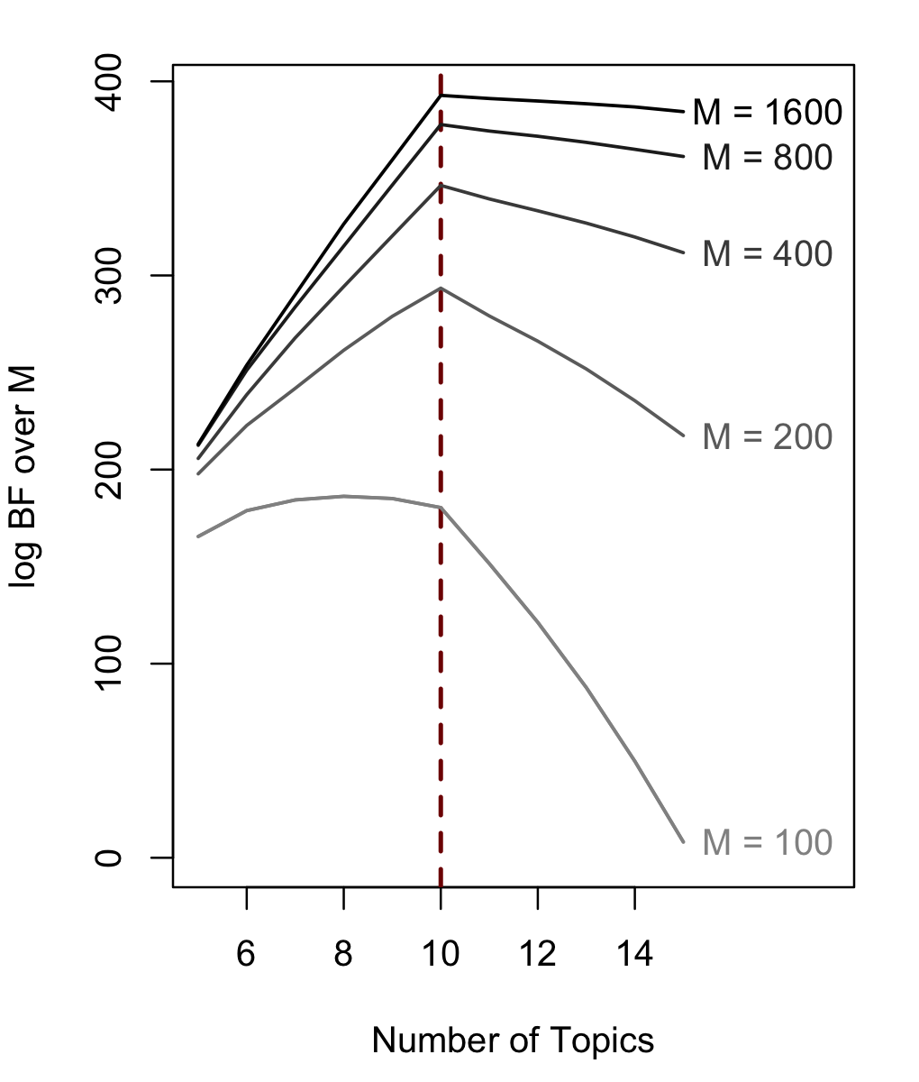
(a)                 (b)

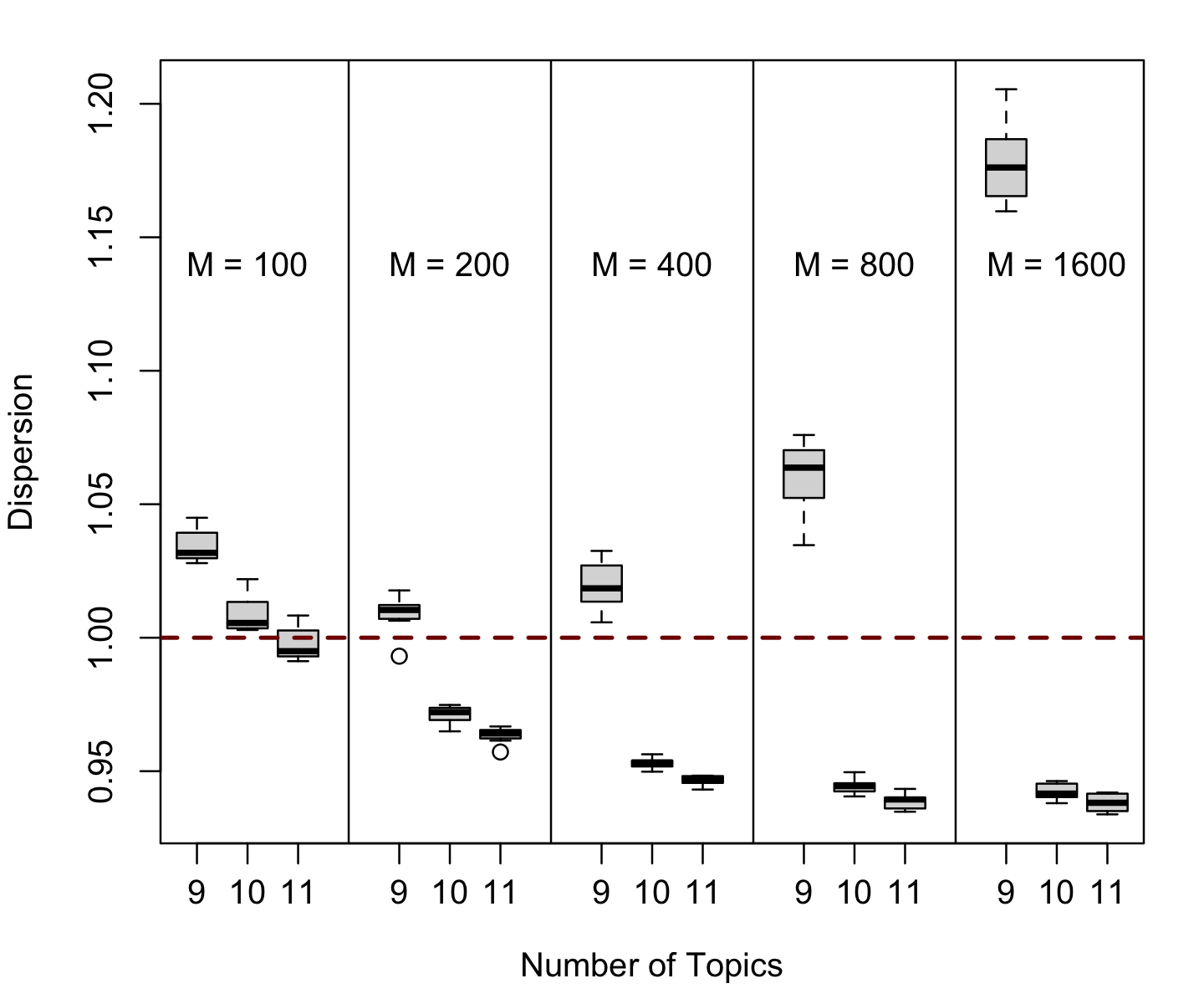
Figure 1: From simulation under various values of $M$, the expected document size, plot (a) shows average log Bayes factors for $K=$ 5-15 against the null one-topic model, and (b) shows estimated dispersion for $K=$ 9-11.

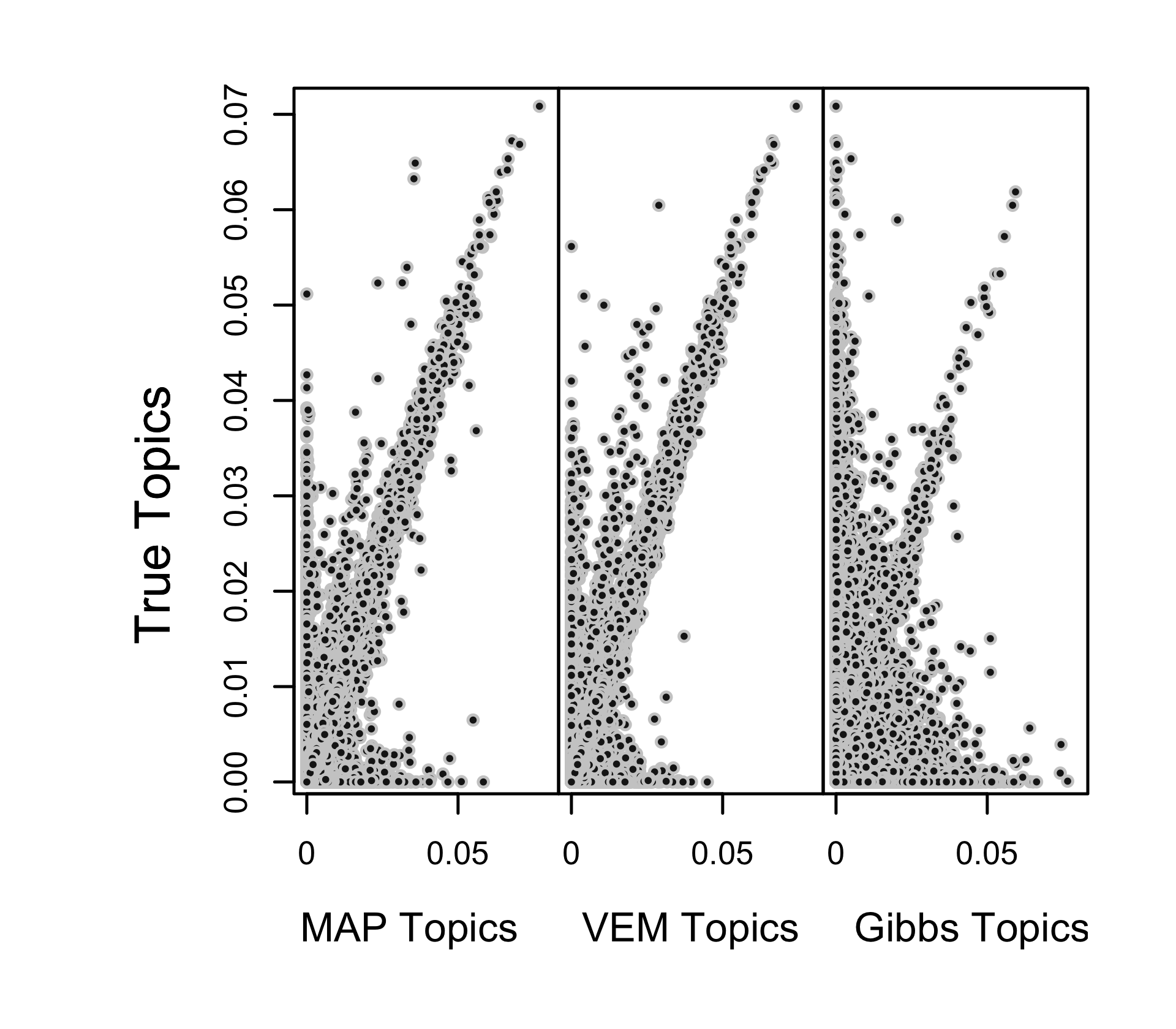
(a)     (b)

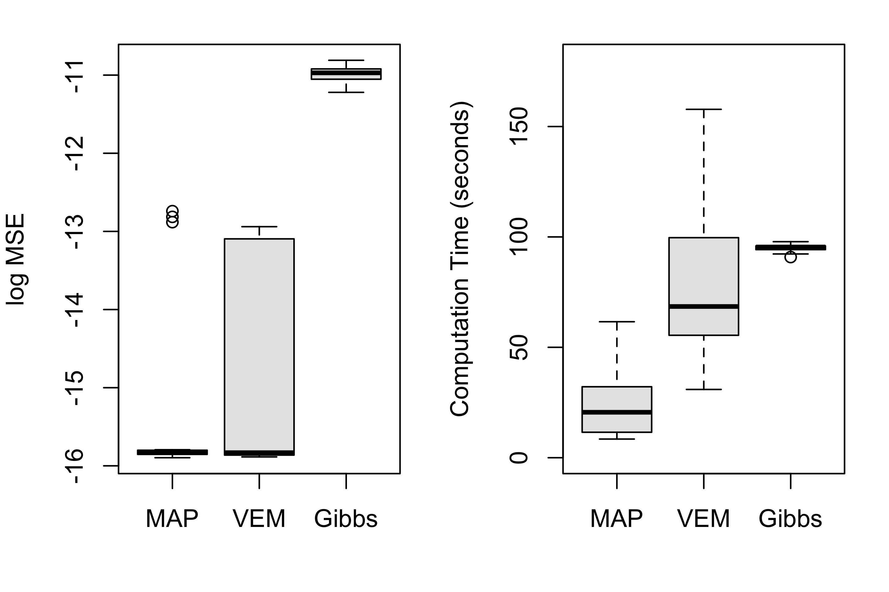
Figure 2: Topic estimation given $K=10$ via MAP, VEM, and Gibbs procedures for data with $M=200$. In (a), elements of each $\boldsymbol{\Theta}$ used in simulation are graphed against the corresponding estimates, and (b) shows the distributions for log MSE of these estimates and for algorithm computation time.

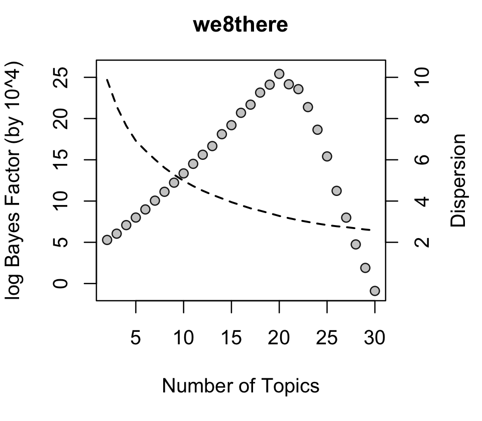
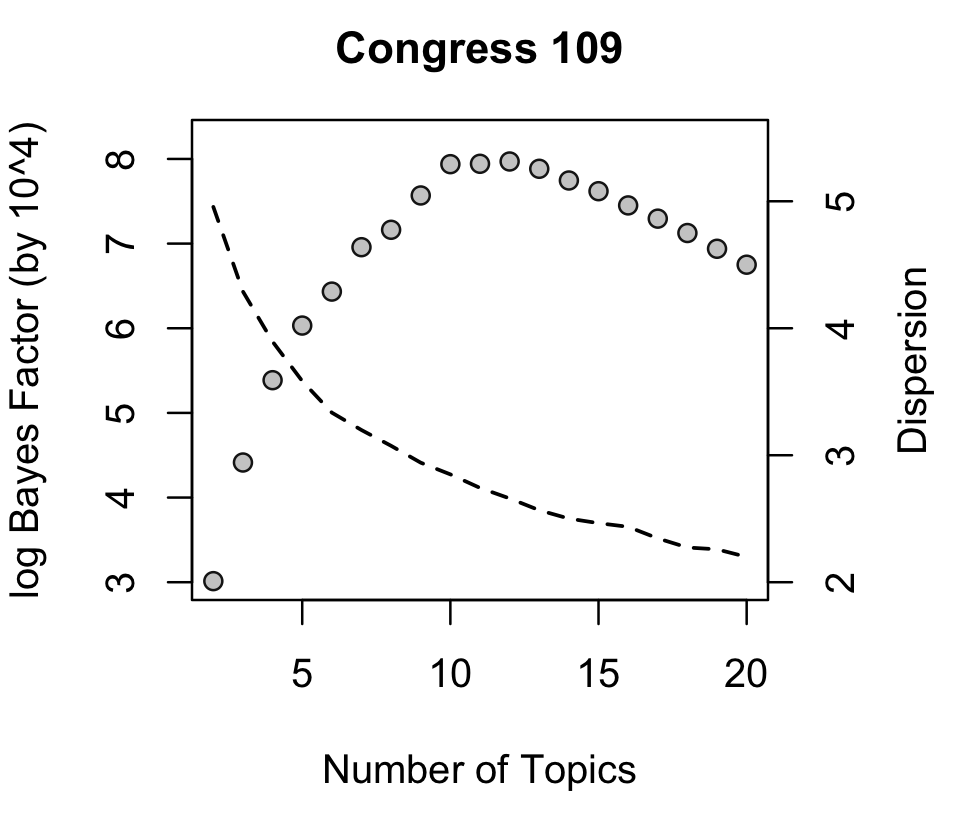
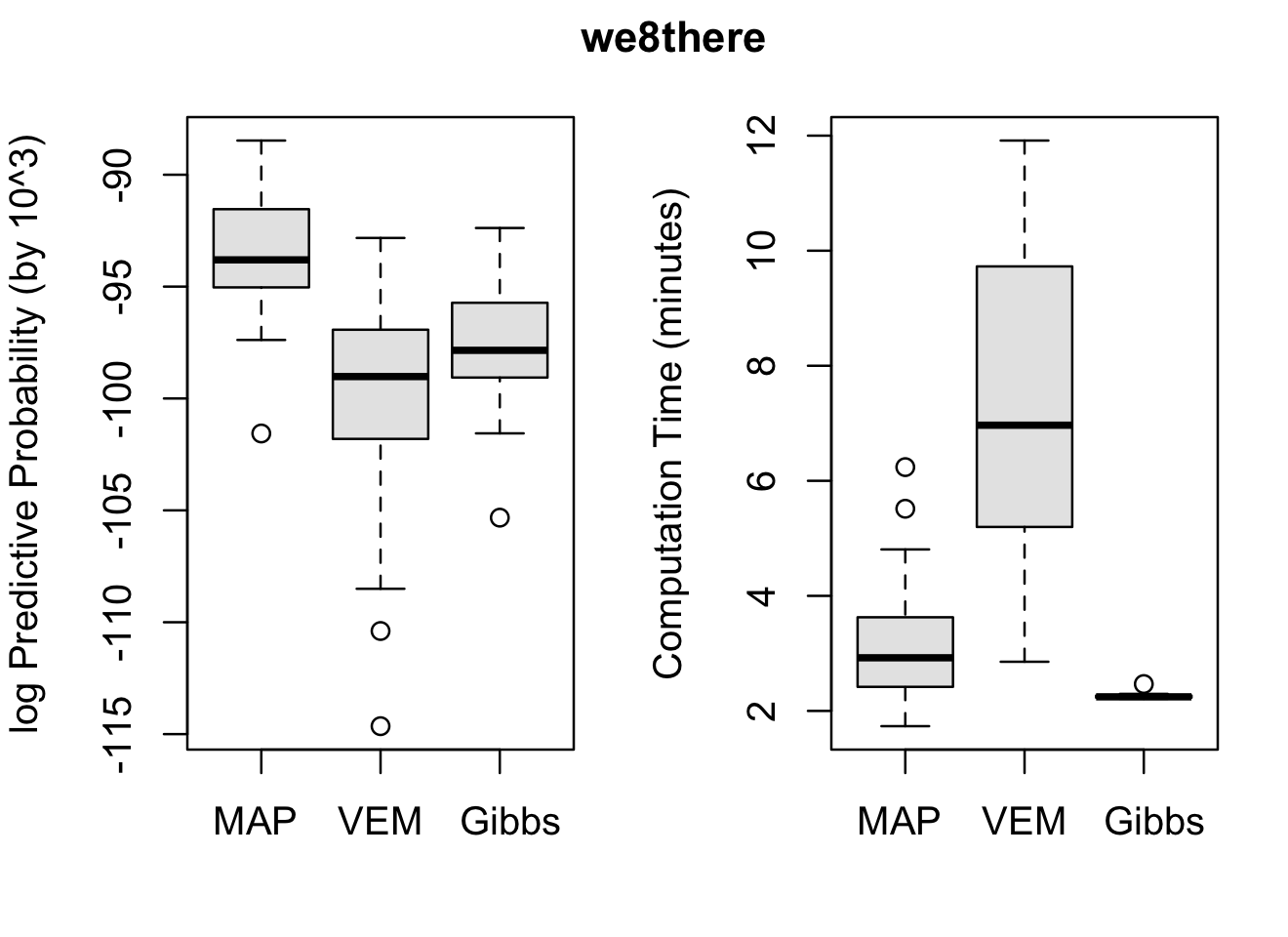
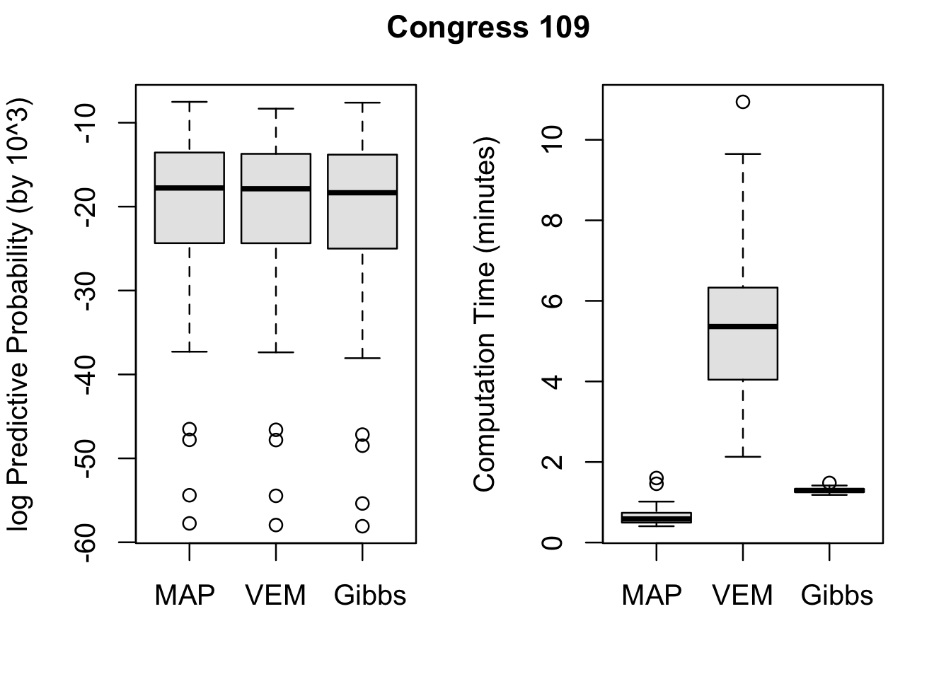
Figure 3: Model selection metrics for each dataset over a range of possible $K$. In each case, the plotted points are log Bayes factor in multiples of $10^{4}$ and the dashed line is estimated dispersion.

Figure 4: Out-of-sample performance for 50 repetitions training on 80% of data and validating on the left-out 20%, with predictive $\sum_{ij}x_{ij}\log(\boldsymbol{\theta}^{\prime}_{\bullet j}\boldsymbol{\omega}_{i})$ in multiples of $10^{3}$ and computation time in minutes.

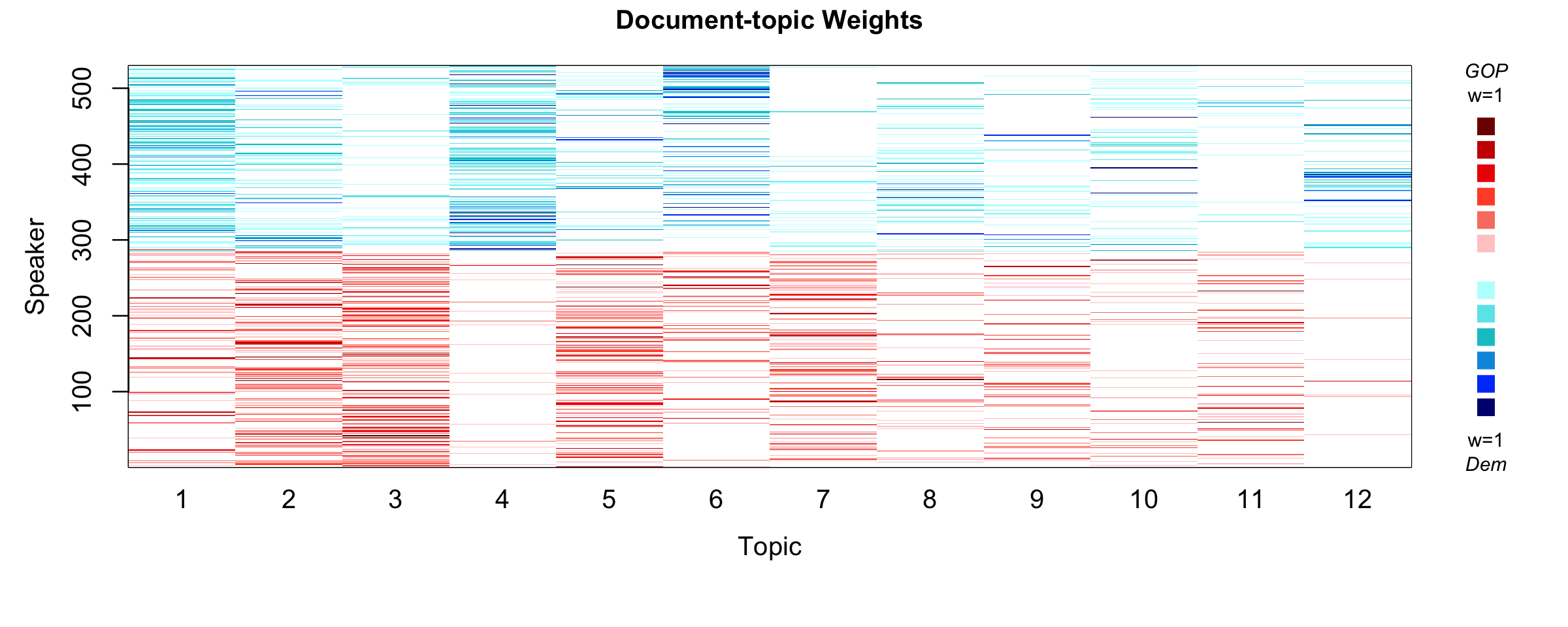
1. dropout.prevention.program, american.force.radio, national.endowment.art, head.start, flood.insurance.program (0.12) 2. near.earth.object, republic.cypru, winning.war.iraq, bless.america, troop.bring.home (0.12) 3. near.retirement.age, commonly.prescribed.drug, repeal.death.tax, increase.taxe, medic.liability.crisi (0.12) 4. va.health.care, united.airline.employe, security.private.account, private.account, issue.facing.american (0.11) 5. southeast.texa, temporary.worker.program, guest.worker.program, million.illegal.immigrant, guest.worker (0.11) 6. national.heritage.corridor, asian.pacific.american, columbia.river.gorge, american.heritage.month (0.10) 7. ready.mixed.concrete, driver.education, witness.testify, indian.affair, president.announce (0.08) 8. low.cost.reliable, wild.bird, suppli.natural.ga, arctic.wildlife.refuge, price.natural.ga (0.06) 9. judicial.confirmation.process, fifth.circuit.court, chief.justice.rehnquist, summa.cum.laude, chief.justice (0.05) 10. north.american.fre, american.fre.trade, change.heart.mind, financial.accounting.standard, central.american.fre (0.05) 11. pluripotent.stem.cel, national.ad.campaign, cel.stem.cel, produce.stem.cel, embryonic.stem (0.04) 12. able.buy.gun, deep.sea.coral, buy.gun, credit.card.industry, caliber.sniper.rifle (0.04)

Figure 5: Congress109 topics, summarized as their top-five terms by lift – $\theta_{kj}$ over empirical term probability – and ordered by usage proportion (column-means of $\boldsymbol{\Omega}$, which are included in parentheses). The image plot has cells shaded by magnitude of $\omega_{ik}$, with Republicans in red and Democrats in blue.

5 Examples

Our methods are all implemented in the textir package for R. For comparison, we also consider R-package implementations of VEM (topicmodels 0.1-1, Grün and Hornik, 2011) and collapsed Gibbs sampling (lda 1.3.1, Chang, 2011). Although in each case efficiency could be improved through techniques such as parallel processing or thresholding for sparsity (e.g., see the SparseLDA of Yao et al., 2009), we seek to present a baseline comparison of basic algorithms. The priors of Section 3 are used throughout, and times are reported for computation on a 3.2 GHz Mac Pro.

The original topicmodels code measures convergence on proportional change in the log posterior bound, leading to observed absolute log posterior change of 50-100 at termination under tolerance of $10^{-4}$. Such premature convergence leads to very poor results, and the code (rlda.c line 412) was altered to match textir in tracking absolute change. Both routines then stop on a tolerance of 0.1. Gibbs samplers were run 5000 iterations, and lda provides a single posterior draw for estimation.

5.1 Simulation Study

We consider data simulated from a ten-topic model with $p=1000$ dimensional topics $\boldsymbol{\theta}_{k}\sim\mathrm{Dir}(1/10),~{}k=1,\ldots,10$, where each of $n=500$ documents are generated with weights $\boldsymbol{\omega}_{i}\sim\mathrm{Dir}(1/10)$ and phrase counts $\mathbf{x}_{i}\sim\mathrm{MN}(\boldsymbol{\Theta}\boldsymbol{\omega}_{i},m_{i})$ given $m_{i}\sim\mathrm{Po}(M)$. This yields topics and topic weights that are dominated by a subset of relatively large probability, and we have set sample size at half vocabulary dimension to reflect the common $p>\!\!>n$ setting of text analysis. Expected size, $M$, varies to illustrate the effect of increased information in 5 sets of 50 runs for $M$ from 100 to 1600.

To investigate model selection, we fit $K=5\ldots 15$ topics to each simulated corpus. Figure 2 graphs results. Marginal likelihood estimates are in 2.a as log Bayes factors, calculated over the null model of $K=1$. Apart from the low information $M=100$, mean $\mathrm{p}(\mathbf{X}\mid K)$ is maximized at the true model of $K=10$; this was very consistant across individual simulations, with $K=10$ chosen invariably for $M\geq 200$. Even at $M=100$, where $K=8$ was the most commonly chosen model, the likelihood is relatively flat before quickly dropping for $K>10$. In 2.b, the sample dispersion distribution is shown for $K=9,10,11$ at each size specification. Of primary interest, $\hat{\sigma}^{2}$ is almost always larger than one for $K<10$ and less than one for $K\geq 10$. This pattern persists for un-plotted $K$, and separation across models increases with $M$. Estimated dispersion does appear to be biased low by roughly 1-6% depending on size, illustrating the difficulty of choosing effective degrees of freedom. As a result, our $\chi^{2}$ test of a more-topics-than-$K$ alternative leads to $p$-values of $p=0$ for $K<10$ and $p=1$ for $K\geq 10$.

We then consider MAP, VEM, and Gibbs estimation for the true $K=10$ model with 50 datasets simulated at $M=200$. To account for label-switching, estimated topics were matched with true topics by pairing the $\boldsymbol{\Theta}$ columns of least sum squared difference. Results are shown in Figure 2. The plots in 2.a show largely accurate estimation for both VEM and MAP procedures, but with near-zero $\theta$ occasionally fit at large $\hat{\theta}$ and vice versa. This occurs when some vocabulary probabilities are swapped in estimation across topics, an event that is not surprising under the weak identification of our high-dimensional latent variable model. It appears in 2.b that MAP does have slightly lower MSE, even though VEM takes at least 2-3 times longer to converge. Finally, as would be expected of estimates based on a single draw from a short MCMC run, Gibbs MSE are far larger than for either alternative.

5.2 Data Analysis

The data sets we consider are detailed in Taddy (2012) and included as examples in textir. We8there consists of counts for 2804 bigrams in 6175 online restaurant reviews, and Congress109 was compiled by Gentzkow and Shapiro (2010) from the $109^{th}$ US Congress as 529 legislators’ usage counts for each of 1000 bigrams and trigrams pre-selected for partisanship.

Model selection results are in Figure 4. The marginal likelihood surfaces, again expressed as Bayes factors, are maximized at $K=20$ for the we8there data and at $K=12$ for congress109. Interestingly, dispersion estimates remain larger than one for these chosen models, and we do not approach $\hat{\sigma}^{2}=1$ even for $K$ up to $200$. This indicates alternative sources of overdispersion beyond topic-clustering, such as correlation between counts across phrases in a given document.

Working with the likelihood maximizing topic models, we then compare estimators by repeatedly fitting $\boldsymbol{\widehat{\Theta}}$ on a random 80% of data and calculating predictive probability over the left-out 20%. In each case, new document phrase probabilities were calculated as $\boldsymbol{\widehat{\Theta}}\boldsymbol{\omega}_{i}$ using the conditional MAP for $\boldsymbol{\omega}_{i}$ under a $\mathrm{Dir}(1/K)$ prior. Figure 4 presents results. As in simulation, the MAP algorithm appears to dominate VEM: predictive probability is higher for MAP in the we8there example and near identical across methods for congress109, while convergence under VEM takes many times longer. Gibbs sampling is quickly able to find a neighborhood of decent posterior probability, such that it performs well relative to VEM but worse than the MAP estimators.

Finally, to illustrate the analysis facilitated by these models, Figure 5 offers a brief summary of the congress109 example. Top phrases from each topic are presented after ranking by term-lift, $\theta_{kj}/q_{j}$ where $q_{j}=\sum_{i=1}^{n}x_{ij}/\sum_{i=1}^{n}m_{i}$, and the image plots party segregation across topics. Although language clustering is variously ideological, geographical, and event driven, some topics appear strongly partisan (e.g., 3 for Republicans and 4 for Democrats). Top-lift terms in the we8there example show similar variety, with some topics motivated by quality, value or service:

1. anoth.minut, flag.down, over.minut, wait.over, arriv.after (0.07)

2. great.place, food.great, place.eat, well.worth, great.price (0.06)

while others are associated with specific styles of food:

9. chicago.style, crust.pizza, thin.crust, pizza.place, deep.dish (0.05)

11. mexican.food, mexican.restaur, authent.mexican, best.mexican (0.05).

In both examples, the model provides massive dimension reduction (from 1000 to 12 and from 2804 to 20) by replacing individual phrases with topic weights.

6 Discussion

Results from Section 5 offer some general support for our methodology. In model selection, the marginal likelihood approximation appears to provide for efficient data-driven selection of the number of latent topics. Since a default approach to choosing $K$ has been thus far absent from the literature, this should be of use in the practice of topic modeling. We note that the same block-diagonal Laplace approximation can be applied as a basis for inference and fast posterior interval calculations. Dispersion shows potential for measuring goodness-of-fit, but its role is complicated by bias and alternative sources of overdispersion.

We were pleased to find that the efficiency of joint MAP estimation did not lead to lower quality fit, but rather uniformly met or outperformed alternative estimates. The simple algorithm of this paper is also straightforward to scale for large-data analyses. In a crucial step, the independent updates for each $\boldsymbol{\omega}_{i}|\boldsymbol{\Theta}$ can be processed in parallel; our experience is that this allows fitting 20 or more topics to hundreds of thousands of documents and tens of thousands of unique terms in less than ten minutes on a common desktop.

References

- Airoldi et al. (2010) Airoldi, E. M., E. A. Erosheva, S. E. Fienberg, C. Joutard, T. Love, and S. Shringarpure (2010). Reconceptualizing the classification of pnas articles. Proceedings of the National Academy of Sciences 107, 20899—20904.
- Alexander et al. (2009) Alexander, D. H., J. Novembre, and K. Lange (2009). Fast model-based estimation of ancestry in unrelated individuals. Genome Research 19, 1655–1664.
- Asuncion et al. (2009) Asuncion, A., M. Welling, P. Smyth, and Y. W. Teh (2009). On smoothing and inference for topic models. In Proceedings of the Twenty-Fifth Conference on Uncertainty in Artificial Intelligence. UAI.
- Berger et al. (1999) Berger, J. O., B. Liseo, and R. L. Wolpert (1999). Integrated likelihood methods for eliminating nuissance parameters. Statistical Science 14, 1–28.
- Blei and Lafferty (2006) Blei, D. M. and J. D. Lafferty (2006). Dynamic topic models. In Proceedings of the 23rd International Conference on Machine Learning. ICML.
- Blei and Lafferty (2007) Blei, D. M. and J. D. Lafferty (2007). A correlated topic model of Science. The Annals of Applied Statistics 1, 17–35.
- Blei and McAuliffe (2010) Blei, D. M. and J. D. McAuliffe (2010). Supervised topic models. arXiv:1003.0783v1.
- Blei et al. (2003) Blei, D. M., A. Y. Ng, and M. I. Jordan (2003). Latent Dirichlet allocation. Journal of Machine Learning Research 3, 993–1022.
- Chang (2011) Chang, J. (2011). lda: Collapsed Gibbs sampling methods for topic models. R package version 1.3.1.
- Deerwester et al. (1990) Deerwester, S., S. T. Dumais, G. W. Furnas, T. K. Landauer, and R. Harshman (1990). Indexing by latent semantic analysis. Journal of the American Society for Information Science 41, 391–407.
- Gentzkow and Shapiro (2010) Gentzkow, M. and J. Shapiro (2010). What drives media slant? Evidence from U.S. daily newspapers. Econometrica 78, 35–72.
- Griffiths and Styvers (2004) Griffiths, T. L. and M. Styvers (2004). Finding scientific topics. In Proceedings of the National Acadamy of Sciences, Volume 101, pp. 5228–5235. PNAS.
- Grimmer (2010) Grimmer, J. (2010). A Bayesian hierarchical topic model for political texts: Measuring expressed agendas in senate press releases. Political Analysis 18, 1–35.
- Grün and Hornik (2011) Grün, B. and K. Hornik (2011). topicmodels: An R package for fitting topic models. Journal of Statistical Software 40, 1–30.
- Haberman (1973) Haberman, S. J. (1973). The analysis of residuals in cross-classified tables. Biometrics 29, 205–220.
- Hastie et al. (2009) Hastie, T., R. Tibshrani, and J. H. Friedman (2009). The Elements of Statistical Learning. Springer.
- Hofmann (1999) Hofmann, T. (1999). Probabilistic latent semantic indexing. In Proceedings of the Twenty-Second Annual International SIGIR Conference.
- Ipsen and Lee (2011) Ipsen, I. and D. Lee (2011). Determinant approximations. http://arxiv.org/abs/1105.0437v1.
- Kass and Raftery (1995) Kass, R. E. and A. E. Raftery (1995). Bayes factors. Journal of the American Statistical Association 90, 773–795.
- Lange (2010) Lange, K. (2010). Numerical Analysis for Statisticians (2nd ed.). Springer.
- Luenberger and Ye (2008) Luenberger, D. G. and Y. Ye (2008). Linear and Nonlinear Programming (3rd ed.). Springer.
- Mackay (1998) Mackay, D. (1998). Choice of basis for laplace approximation. Machine Learning 33, 77–86.
- Neal (2000) Neal, R. (2000). Markov chain sampling methods for Dirichlet process mixture models. Journal of Computational and Graphical Statistics 9, 249–265.
- Pritchard et al. (2000) Pritchard, J. K., M. Stephens, and P. Donnelly (2000). Inference of polulation structure using multilocus genotype data. Genetics 155, 945–959.
- Roeder and Wasserman (1997) Roeder, K. and L. Wasserman (1997). Practical Bayesian density estimation using mixtures of normals. Journal of the American Statistical Association 92, 894–902.
- Taddy (2012) Taddy, M. A. (2011). Inverse regression for analysis of sentiment in text. Submitted. http://arxiv.org/abs/1012.2098.
- Tang et al. (2006) Tang, H., M. Coram, P. Wang, X. Zhu, and N. Risch (2006). Reconstructing genetic ancestry blocks in admixed individuals. American Journal of Human Genetics 79, 1–12.
- Teh et al. (2006) Teh, Y. W., M. I. Jordan, M. J. Beal, and D. M. Blei (2006). Hierarchical Dirichlet processes. Journal of the American Statistical Association 101, 1566–1581.
- Teh et al. (2006) Teh, Y. W., D. Newman, and M. Welling (2006). A collapsed variational Bayesian inference algorithm for latent Dirichlet allocation. In Neural Information Processing Systems, pp. 1–8. NIPS.
- Tierney and Kadane (1986) Tierney, L. and J. B. Kadane (1986). Accurate approximations for posterior moments and marginal densities. Journal of the American Statistical Association 81, 82–86.
- Wainwright and Jordan (2008) Wainwright, M. J. and M. I. Jordan (2008). Graphical models, exponential families, and variational inference. Foundations and Trends in Machine Learning 1, 1–305.
- Wallach et al. (2009) Wallach, H. M., D. Mimno, and A. McCallum (2009). Rethinking LDA: Why priors matter. In Neural Information Processing Systems. NIPS.
- Yao et al. (2009) Yao, L., D. Mimno, and A. McCallum (2009). Efficient methods for topic model inference on streaming document collections. In 15th Conference on Knowledge Discovery and Data Mining.