Simulating Gyrokinetic Microinstabilities in Stellarator Geometry with GS2

Abstract

The nonlinear gyrokinetic code GS2 has been extended to treat non-axisymmetric stellarator geometry. Electromagnetic perturbations and multiple trapped particle regions are allowed. Here, linear, collisionless, electrostatic simulations of the quasi-axisymmetric, three-field period National Compact Stellarator Experiment (NCSX) design QAS3-C82 have been successfully benchmarked against the eigenvalue code FULL. Quantitatively, the linear stability calculations of GS2 and FULL agree to within $\sim 10\%$.

I Introduction

One of the most important issues for magnetic fusion is the confinement of heat and particles. Turbulent transport (most likely the result of drift wave instabilities) causes a significant amount of heat loss in tokamaks and spherical tori.Liewer (1985) Neoclassical transport, on the other hand, can often account for the poor confinement in traditional stellarators.Fu et al. (2007) However, modern stellarator designs, such as Wendelstein 7-AS (W7-AS),Sapper and Renner (1990) Wendelstein 7-X (W7-X),Beidler et al. (1990); Grieger et al. (1992) the National Compact Stellarator Experiment (NCSX),Zarnstorff et al. (2001) the Large Helical Device (LHD) Yamada et al. (2001), and the Helically Symmetric Experiment (HSX) Gerhardt et al. (2005); Canik et al. (2007); Talmadge et al. (2008) have shown or are designed to have improved neoclassical confinement and stability properties. Understanding plasma turbulence and transport could further improve the performance of stellarators. Progress in design of stellarators for optimal transport has been made by coupling the gyrokinetic code GENEJenko et al. (2000) with the configuration optimization code STELLOPT.Mynick, Pomphrey, and Xanthopoulos (2010); Reiman et al. (1999)

Gyrokinetic studies of drift-wave-driven turbulence in stellarator geometry are relatively recent and comprehensive scans are scarce. Most of these studies were done using upgraded versions of well-established axisymmetric codes which include comprehensive kinetic dynamics (multispecies, collisions, finite beta) to the more general case of non-axisymmetric stellarator geometry, in the flux tube limit. The first non-axisymmetric linear gyrokinetic stability studies, for both the ion-temperature-gradient-driven (ITG) mode and the trapped-electron mode (TEM), were done with the linear eigenvalue FULL code,Rewoldt, Tang, and Chance (1982); Rewoldt, Tang, and Hastie (1987); Rewoldt et al. (1999) including a comparison of stability in nine stellarator configurations.Rewoldt, Ku, and Tang (2005) Extensive studies have been done with the upgraded GENE code, including the first nonlinear gyrokinetic simulations.Xanthopoulos et al. (2007) More recently, the GKV-X code, which uses the adiabatic electron approximation, has been used to analyze linear ITG modes and zonal flows in LHD and nonlinear studies are in progress.Watanabe, Sugama, and Ferrando-Margalet (2007)

For this purpose, the axisymmetric nonlinear microinstability code GS2Dorland et al. (2000) has been extended to treat the more general case of non-axisymmetric stellarator geometry. GS2 contains a full (except that the equilibrium distribution function is taken to be a Maxwellian) implementation of the 5-D Frieman and Chen nonlinear gyrokinetic equation in the flux tube limit,Dorland et al. (2000); Howes et al. (2006) with an efficient parallelization for modern supercomputers.Kotschenreuther, Rewoldt, and Tang (1995) It treats electrons and an arbitrary number of ion species on an equal footing, and includes trapped particles, electromagnetic perturbations, and a momentum-conserving pitch-angle-scattering collision operator. The extension of the code to non-axisymmetric geometry not only retains all of the above dynamics of the axisymmetric version, but also allows, most importantly, multiple trapped particle regions and multiple totally-trapped pitch angles at a given theta grid point. (By “totally-trapped,” we mean particles with such a small parallel velocity that they are limited to one grid point at the bottom of a well.) Tokamaks only have one trapped particle region, but as stellarators can have many deep, narrow magnetic wells which can trap particles (though NCSX has only a single deep well, with other shallow wells, and is a bridge in configuration space between tokamaks and other stellarators). In order to treat the trapped particles accurately, one needs to resolve these wells sufficiently with high grid resolution. With the GS2 modifications, we allow for more flexible, decoupled pitch angle and parallel spatial grids, relative to the original GS2 algorithm which required every grid point ($\theta_{j}$) along the field line to correspond exactly to the turning point of trapped pitch angle ($\lambda_{i}=\mu/E$) grid points.Kotschenreuther, Rewoldt, and Tang (1995)

Beyond these extensions, a GS2 stellarator simulation requires different geometry codes to build its input grids than standard tokamak runs. For these non-axisymmetric simulations, the geometrical coefficients are based on a VMECHirshman, Schwenn, and Nührenberg (1990); Hirshman and Lee (1986) 3D MHD equilibrium, which is transformed into Boozer coordinatesBoozer (1980) by the TERPSICHORE code.Anderson (1990) From this equilibrium, the VVBAL codeCooper (1992) constructs data along a chosen field line necessary for the microinstability calculations: $B=|\mathbf{B}|$, the $\nabla\mathbf{B}$ drift, the curvature drift, and the metric coefficients. While these extensions were used to study HSX plasmas,Guttenfelder et al. (2008) here we verify the non-axisymmetric extension of GS2 through comparisons with FULL on NCSX plasmas. Good agreement between the GS2 code and the FULL code in the axisymmetric limit has been extensively demonstrated previously.Kotschenreuther, Rewoldt, and Tang (1995); Bourdelle et al. (2003) While the non-axisymmetric upgrade of GS2 retains the nonlinear dynamics, in these studies we focus on systematic scans of gyrokinetic linear stability.

The organization of this paper is as follows. The NCSX equilibrium used for the benchmark is described in Section II. Comparisons between the GS2 code and the FULL code in non-axisymmetric geometry over a range of parameters including $\eta=L_{n}/L_{T}$ (where $L_{n}$ is the density gradient scale length and $L_{T}$ is the temperature gradient scale length), $k_{y}\rho_{i}$, $T_{i}/T_{e}$, and geometrical coordinates are presented in Section III. Further results using the GS2 code to investigate effects of density and temperature gradients are presented in Section IV. Conclusions and a discussion of future work are given in Section V. Finally, Appendix A contains definitions of the normalizations and radial coordinate used by GS2.

II The QAS3-C82 Equilibrium

All of the benchmark calculations use a VMEC equilibrium based on a 1999 NCSX design known as QAS3-C82,Reiman et al. (1999) which is shown in Figure 1. This configuration is quasi-axisymmetric with three field periods. It has an aspect ratio of 3.5 and a major radius of 1.4 m. NCSX was designed to have good neoclassical transport and MHD stability properties and good drift trajectories similar to those in tokamaks. Strong axisymmetric components of shaping provide good ballooning stability properties at lower aspect ratio. Furthermore, the QAS3-C82 equilibrium has a monotonically increasing rotational transform profile which provides stability to neoclassical tearing modes across the entire cross section.Reiman et al. (2001, 1999)

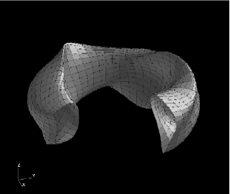
Figure 1: Equilibrium of NCSX design QAS3-C82 which is quasi-axisymmetric and has 3 field periods.

For most of these runs, we chose the surface at $s=0.875$ ($s\sim\langle(r/a)^{2}\rangle$ is the normalized toroidal flux) and the field line at $\alpha=\pi/3$ ($\alpha=\zeta-q\theta$; $\zeta$ is the Boozer toroidal angle, $\theta$ is the Boozer poloidal angle). The cross-section at this point is the crescent shape, seen in Figure 17 of Ref. Ku and Boozer, 2010. The coordinate along the field line is $\theta$, the poloidal angle. At this surface, the safety factor $q=2.118$ and the average $\beta$ (the ratio of the plasma pressure to the magnetic pressure) is $\langle\beta\rangle=0.01\%$. Lastly, the ballooning parameterCooper (1992) is $\theta_{0}=0$, except in Figure 6.

Figure 2 shows the variation of the magnitude of the magnetic field along a chosen magnetic field line. Resolution studies for the spatial grid used in the GS2 runs indicate that 330 theta grid points per poloidal period and about 90 pitch angles ($\lambda=\mu/E$) showed convergence in the growth rate to within $2\%$, however $<10\%$ error is possible with coarser grids. It was also found that a $\theta$ range extending from $-3\pi$ to $3\pi$ was sufficient for a typical simulation grid, meaning that the eigenfunctions for the modes decayed to insignificant values before reaching these boundaries. (The endpoints of $B(\theta)$ were increased slightly, by less than $1\%$, to be global maxima, per normal GS2 operations.)

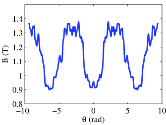
Figure 2: Standard B vs. $\theta$ grid for QAS3-C82, with $s=0.875$, $\alpha=\pi/3$, and $\theta_{0}=0$.

The equilibrium’s geometry suggests unstable drift waves exist. The variations of $(k_{\perp}/n)^{2}$, where $n$ is the toroidal mode number, and the curvature drift along the same chosen field line can be seen in Figures 3 and 4. By convention, positive curvature drifts are “bad” or destabilizing, while negative curvature drifts are “good” or stabilizing. Significant unstable modes occur where $k_{\perp}$ is small, which is near $\theta=0$ for this equilibrium, since instabilities are generally suppressed at large $k_{\perp}$ by FLR averaging. Also, because Figure 4 indicates that the curvature is bad in this region near $\theta=0$, it is expected that unstable modes will appear here.

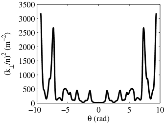
Figure 3: Variation of $(\frac{k_{\perp}}{n})^{2}(\theta)$ for QAS3-C82, with $s=0.875$, $\alpha=\pi/3$, and $\theta_{0}=0$.

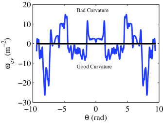
Figure 4: Variation of the curvature drift frequency ($\omega_{cv}=(\mathbf{k_{\perp}}/n)\cdot\mathbf{b}\times[\mathbf{b}\cdot\nabla\mathbf{b}]$) (for $n=1$) along $\theta$ for QAS3-C82, with $s=0.875$, $\alpha=\pi/3$, and $\theta_{0}=0$.

III Benchmarks with FULL

Comparisons between the GS2 code and the FULL code in non-axisymmetric geometry over a range of parameters using the QAS3-C82 equilibrium show linear agreement for our standard case, whose local parameters are shown in Table I. The product of the perpendicular wave number and the gyroradius at $\theta=0$, $k_{y}\rho_{i}$, is $0.3983$ (where the toroidal mode number $n=25$; see App. A) for all cases unless otherwise specified. The standard case is relatively close to the edge, which accounts for the low values of ion temperature, $T_{i}$, electron temperature, $T_{e}$, and relatively large values for the gradients. The parameter, $\eta=L_{n}/L_{T}$ is usually $\eta=3$, placing most of our studies in an ITG regime (see Figure 7). Correspondingly, $a_{N}/L_{ni}=a_{N}/L_{ne}=13.096$ and $a_{N}/L_{Ti}=a_{N}/L_{Te}=39.288$. The major radius is approximately $R\approx 1.4m$. The normalizing scale length is $a_{N}=n/k_{\perp}(\theta=0)=0.352m$, not the minor radius, and is described in detail in App. A. These studies are done with electrons and deuterium ions.

$s\approx\left(\langle r/a\rangle\right)^{2}$	$0.875$
$\alpha=\zeta-q\theta$	$\pi/3$
$\theta_{0}$	$0$
$q$	$2.118$
$\langle\beta\rangle$	$0.01\%$
$k_{y}\rho_{i}$	$0.3983$$(n=25)$
$T_{i}=T_{e}$	$1keV$
$\eta_{i}=\eta_{e}$	$3$
$a_{N}/L_{ni}=a_{N}/L_{ne}$	$\approx 13.096$
$a_{N}/L_{Ti}=a_{N}/L_{Te}$	$\approx 39.288$
$R$	$\approx 4a_{N}\approx 1.4m$
$a_{N}=(\frac{n}{k_{\perp}(\theta=0,\theta_{0}=0)})$	$\approx 0.352m$
$B_{a}=\langle B\rangle$	$1.15T$
$m_{ref}$	$2m_{p}$
$v_{t}$	$\sqrt{(eT_{i}1000)/m_{ref}}$
GS2 $\omega$ units $v_{t}/a_{N}$	$\approx 6.214\times 10^{5}sec^{-1}$

Table 1: The set of local parameters used in a standard case microinstability simulation based on the QAS3-C82 equilibrium. Note: $a_{N}$ is not the minor radius; it is discussed in App. A.

Previously, FULL scans showed that the largest linear growth rate occurs at flux surface label $s=0.875$ (corresponding to a minor radius of $r/a\approx\sqrt{s}\approx 0.94$), for $\alpha=\pi/3$ and $\theta_{0}=0$. GS2 and FULL scans over $\alpha$ and $\theta_{0}$ (Figures 5 and 6) adopted this $s$ value. The toroidal mode number, $n$, was fixed at $25$ (thus, $k_{y}\rho_{i}=\frac{n}{a_{N}}\rho_{i}$ varied for each data point, because from App. A, $a_{N}=1/|\nabla\alpha|$ and $\rho_{i}\propto 1/B_{a}$ vary). These figures indicate good agreement between the GS2 code and the FULL code. The maximum growth rate in Figure 5 occurs for $\alpha=\pi/3$, and GS2 and FULL agree well around this value. In Figure 6, GS2 and FULL again agree well around the growth rate peak at $\theta_{0}=0$.

In all further calculations presented in this paper, $s=0.875$, $\alpha=\pi/3$ and $\theta_{0}=0$, the location of the maximum growth rate.

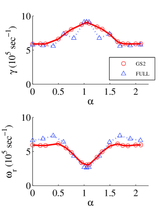
Figure 5: (color online) Variation of $\gamma$ and $\omega_{r}$ with $\alpha$ at constant $s=0.875$ and $\theta_{0}=0$ with $\eta_{i}=\eta_{e}=3$ and $k_{y}\rho_{i}(\alpha=\frac{\pi}{3})=0.3983$.

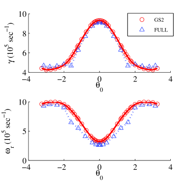
Figure 6: (color online) Variation of $\gamma$ and $\omega_{r}$ with $\theta_{0}$ at constant $s=0.875$ and $\alpha=\pi/3$ with $\eta_{i}=\eta_{e}=3$ and $k_{y}\rho_{i}=0.3983$.

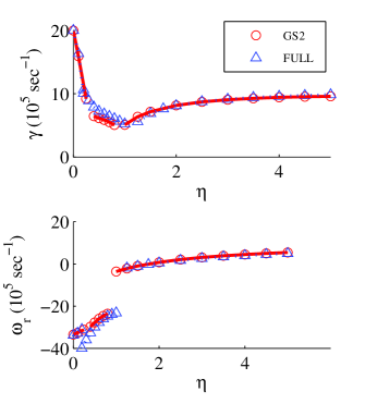
Figure 7: (color online) Variation of $\gamma$ and $\omega_{r}$ with $\eta_{i}=\eta_{e}$ with $k_{y}\rho_{i}=0.3983$.

We used GS2 to find the instability growth rate dependence on $\eta=L_{n}/L_{T}$ and compared it with FULL. The total pressure gradient was kept fixed to maintain consistency with the MHD equilibrium. Both codes found large growth rates at low $\eta$ (high density gradient) and high $\eta$ (high temperature gradient) (Figure 7), and agree well, though it can be seen in the frequencies that GS2 found a mode switch earlier than FULL. This can happen since GS2 automatically finds the most unstable mode, whereas FULL usually finds the mode closest to the initial guess provided to the root finder. In fact, there are three distinct eigenmodes within these regimes of $\eta$: at small $\eta$, even-symmetry TEM modes dominate; at medium $\eta$, odd-symmetry TEM modes dominate; and at larger values of $\eta$, an even-symmetry ITG-driven mode dominatesRewoldt et al. (1999) (Figure 8). This is typical of an equivalent axisymmetric configuration.Rewoldt and Tang (1990)

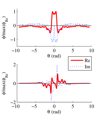
Figure 8: (color online) Variation of the normalized GS2 eigenfunctions of electrostatic, collisionless toroidal drift modes along the field line at $\eta=3$ (top figure) and at $\eta=0.5$ (bottom figure) with $k_{y}\rho_{i}=0.3983$.

Benchmarks with FULL for scans over $T_{i}/T_{e}$, shown in figure 9, were also successful. For this scan, $T_{e}$ was varied while $T_{i}$ was kept constant at $1keV$. As $T_{i}/T_{e}$ increases, at this very large value of $R/L_{T_{i}}\approx 157$, the linear growth rate falls slowly due, most likely, to an enhancement of shielding by adiabatic electrons at large $\sqrt{T_{i}/T_{e}}$. This is a very well-known phenomenon in tokamaks.

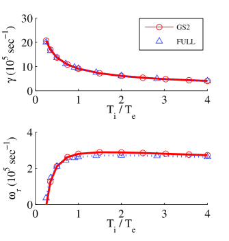
Figure 9: (color online) Variation of $\gamma$ and $\omega_{r}$ with $T_{i}/T_{e}$ with $k_{y}\rho_{i}=0.3983$ and $\eta_{i}=\eta_{e}=3$.

Comparison scans over $k_{y}\rho_{i}$ for $\eta=0$ and $\eta=3$ are shown in figure 10. For the $\eta=0$ curve, the dominating eigenmodes are even in the ranges $0.1<k_{y}\rho_{i}<0.2$ and $0.6<k_{y}\rho_{i}<1.1$. Overall, the results from the GS2 code and the FULL code agree well; growth rates differ by at most $\sim 10\%$ except at transitions between modes.

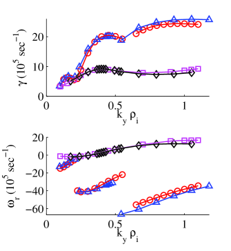
Figure 10: (color online) Variation of $\gamma$ and $\omega_{r}$ with $k_{y}\rho_{i}$. Circles: GS2, $\eta=0$; triangles: FULL, $\eta=0$; squares: GS2, $\eta=3$; diamonds: FULL, $\eta=3$.

We found high frequency, electron-temperature-gradient-driven (ETG) modes with GS2 at short wavelengths (Figure 11) in the extended $k_{y}\rho_{i}$ spectrum for the case of $\eta=3$. This was not checked with FULL.

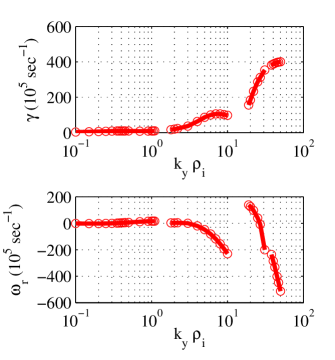
Figure 11: (color online) Extended variation from GS2 of $\gamma$ and $\omega_{r}$ with $k_{y}\rho_{i}$ and $\eta_{i}=\eta_{e}=3$.

IV Critical Gradients for Linear Instability

GS2 was also used to search for critical density gradients and temperature gradients; i.e. to see whether gradients exist at which all drift wave modes are stabilized. Note that for the next series of figures, the normalizing length for the density and temperature gradient length scales is defined as $a_{N}=(n/k_{\perp})(\theta=0)\sim 0.352m$ (see App. A).

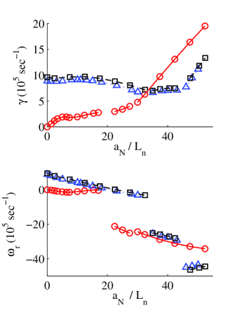
Figure 12: (color online) Variation of $\gamma$ and $\omega_{r}$ with $a_{N}/L_{n}$ with $k_{y}\rho_{i}=0.3983$. Circles: $a_{N}/L_{T}=0.0$; triangles: $a_{N}/L_{T}=39.3$; squares: $a_{N}/L_{T}=44.9$.

Figure 12 shows a scan over the density gradient at various ion and electron temperature gradients. The results are inconsistent with the equilibrium pressure gradient, as the density gradient was increased at constant temperature gradient. However, because the equilibrium beta is so small ($\sim 0.01\%$), the effect of the variation of the pressure gradient is negligible. We see that there is no nonzero critical density gradient threshold, even in the absence of temperature gradients. There are switches in eigenmode symmetry from even to odd as $a_{N}/L_{n}$ increases, or all $a_{N}/L_{T}$ values.

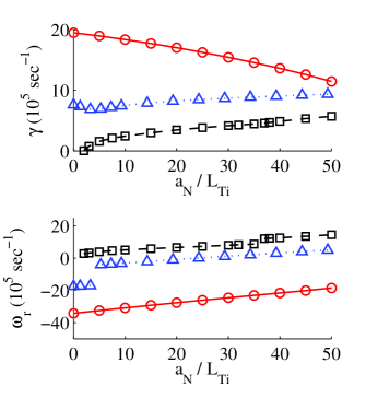
Figure 13: (color online) Variation from GS2 of $\gamma$ and $\omega_{r}$ with $a_{N}/L_{Ti}$ with $k_{y}\rho_{i}=0.3983$. Circles: $a_{N}/L_{n}=52.4,a_{N}/L_{Te}=0.0$; triangles: $a_{N}/L_{n}=13.1,a_{N}/L_{Te}=39.3$; squares: $a_{N}/L_{n}=0.0,a_{N}/L_{Te}=0.0$.

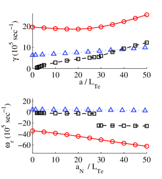
Figure 14: (color online) Variation from GS2 of $\gamma$ and $\omega_{r}$ with $a_{N}/L_{Te}$ for the case of Fig. 2 with $k_{y}\rho_{i}=0.3983$. Circles: $a_{N}/L_{n}=52.4,a_{N}/L_{Ti}=0.0$; triangles: $a_{N}/L_{n}=13.1,a_{N}/L_{Ti}=39.3$; squares: $a_{N}/L_{n}=0.0,a_{N}/L_{Ti}=0.0$.

However, a critical ion temperature gradient for an ITG-driven mode was found at $a_{N}/L_{Ti}\sim 2$ (or $\frac{R}{L_{T_{i}}}=\frac{R}{a_{N}}\frac{a_{N}}{L_{T_{i}}}\approx 4\frac{a_{N}}{L_{T_{i}}}=8$) in the absence of all other gradients (Figure 13). Likewise, a critical electron temperature gradient for a TEM-driven mode was found at $\frac{a_{N}}{L_{T_{e}}}\sim 2$ in the absence of all other gradients (Figure 14).

V Conclusions

The nonlinear gyrokinetic code GS2 has been extended to treat non-axisymmetric stellarator geometry. Geometric quantities required for the gyrokinetic simulations are calculated from a VMEC-generated equilibrium using the VVBAL code and are further described in App. A.

Linear, collisionless, electrostatic simulations of the quasi-axisymmetric, three-field period NCSX stellarator design QAS3-C82 have been successfully benchmarked with the eigenvalue code FULL for scans over a range of parameters including $\eta$, $k_{y}\rho_{i}$, $T_{i}/T_{e}$, $\alpha$, and $\theta_{0}$. Quantitatively, the linear stability calculations of GS2 and FULL agree to within about $10\%$ of the mean, except at transitions between modes. Further results using only GS2 included short wavelength modes, odd parity, faster growing modes, and the effect of individual density and temperature gradients.

Future work will include the exploration of the effects of collisionality and electromagnetic dynamics, investigation of finite beta equilibria, and, most significantly, the effects of nonlinear dynamics. A benchmark of stellarator studies is underway between GS2 and the continuum gyrokinetic code GENEJenko et al. (2000) for NCSX, as well as stellarators W7-AS and W7-X.

GISTXanthopoulos et al. (2009) is now capable of creating GS2 geometry data files and will be used in the future, along with the new GS2 grid generator.

Appendix A Geometry Details

In order to make the simulation grid for these GS2 stellarator runs, VMEC creates the 3-D MHD equilibrium, TERPSICHORE transforms it into Boozer coordinates, and VVBAL calculates necessary geometric coefficients along a specified field line. Then, GS2’s grid generator, Rungridgen, creates the final grid for use in the microinstability calculations. (A new grid generator is in production, which will be used for further GS2 stellarator calculations.) The normalizations of geometric quantities change between these codes, and knowing them in detail is required for benchmarks between gyrokinetic codes. We define the normalizing length, $a_{N}$, in App. A.2.

In GS2, the field-aligned coordinate system is $(\rho,\alpha,\theta)$. $\theta$ is the poloidal angle and distance along the field line. The magnetic field takes the form $\mathbf{B}=\nabla\alpha\times\nabla\Psi$, where $\alpha=\zeta-q\theta$ is the field line label. The radial coordinate, $\rho$, can differ between codes, and we define it in App. A.1. More details of general geometry for GS2 are documented in App. A of Ref. Barnes, 2009.

A.1 Radial coordinate, $\rho$

VMEC and TERPSICHORE use the normalized toroidal flux surface label $s=\Phi/\Phi_{edge}\sim\langle(r/a)^{2}\rangle$ as the radial coordinate, $\rho$. In the customized version of VVBAL used here, the radial coordinate is transformed to $\rho=\Psi_{N}=\Psi/(a_{N}^{2}B_{a})$, where $\Psi_{N}$ is the normalized poloidal flux.

Because Rungridgen uses VVBAL output without modification, here $d\rho/d\psi_{N}\equiv 1$. (In Ref. Barnes, 2009, the definition of the geometry coefficients include the variable $d\rho/d\psi_{N}$, which can be used to choose the radial coordinate.)

A.2 Normalizing Quantities, $B_{a}$ and $a_{N}$

The normalizing magnetic field is $B_{a}=\langle B\rangle$, where $\langle B\rangle$ is a theta-average, not weighted to be a flux-surface average (Ref. Barnes, 2009 chooses $B_{a}$ differently).

The normalizing length is $a_{N}$, given for these calculations by VVBAL as

$$a_{N}=\frac{n}{\sqrt{|\mathbf{k_{\perp}}|^{2}(\theta=0,\theta_{0}=0)}}=\frac{1}{|\nabla\alpha|}.$$ (1)

GS2 treats perturbed quantities as $A=\hat{A}(\theta)exp(iS)$, where $\mathbf{k_{\perp}}=\nabla S=n\nabla(\alpha+q\theta_{0})=n\nabla[\zeta-q(\theta-\theta_{0})]$; $n$ is the toroidal mode number. (In non-axisymmetric devices, $n$ is not a conserved quantum number, because toroidal variations in the equilibrium give coupling between $n$ modes. However, in the small-$\rho*$, high-$n$ limit, this coupling is weak, and $n$ can just be considered a coefficient to select a particular value of $k_{\perp}$.)

In the notation of Eqn. A.11 of App. A in Ref. Barnes, 2009,

$$|\mathbf{k_{\perp}}|^{2}=|\nabla S|^{2}=k_{\theta}^{2}\left|g_{1}+2\theta_{0}g_{2}+\theta_{0}^{2}g_{3}\right|$$ (2)

where $g_{1}$, $g_{2}$, and $g_{3}$ are coefficients in the geometry file written by VVBAL and read by GS2. Also, $k_{\theta}=k_{y}=n/a_{N}$. (The GS2 variable aky is defined as $k_{y}\rho_{i}$, with $\rho_{i}\propto 1/B_{a}$.)

In the notation of Eqn. 7 of Ref. Xanthopoulos et al., 2009,

$$|\mathbf{k_{\perp}}|^{2}=n^{2}\frac{\sqrt{g}B^{2}}{\Psi^{\prime 2}(s)}[C_{p}+C_{s}(\theta-\theta_{0})+C_{q}(\theta-\theta_{0})^{2}],$$ (3)

where $\sqrt{g}$ is the Jacobian, $C_{p}$, $C_{s}$, and $C_{q}$ are defined in section II of Ref. Xanthopoulos et al., 2009.

So, VVBAL writes:

$$g_{1}=a_{N}^{2}\frac{\sqrt{g}B^{2}}{\Psi^{\prime 2}(s)}[C_{p}+C_{s}\theta+C_{q}\theta^{2}]$$ (4)

$$g_{2}=-a_{N}^{2}\frac{\sqrt{g}B^{2}}{\Psi^{\prime 2}(s)}\left[C_{q}\theta+\frac{C_{s}}{2}\right]$$ (5)

$$g_{3}=a_{N}^{2}\frac{\sqrt{g}B^{2}}{\Psi^{\prime 2}(s)}C_{q}$$ (6)

References

- Liewer (1985) P. C. Liewer, Nuclear Fusion 25, 543 (1985).
- Fu et al. (2007) G. Fu, M. Isaev, L. Ku, M. Mikhailov, M. H. Redi, R. Sanchez, A. Subbotin, W. A. Cooper, S. P. Hirshman, D. Monticello, A. Reiman, and M. Zarnstorff, Fusion Science and Technology 51, 218 (2007).
- Sapper and Renner (1990) J. Sapper and H. Renner, Fusion Technology 7, 62 (1990).
- Beidler et al. (1990) C. Beidler, G. Grieger, F. Herrnegger, E. Harmeyer, J. Kisslinger, W. Lotz, H. Maassberg, P. Merkel, J. Nuhrenberg, F. Rau, J. Sapper, F. Sardei, R. Scardovelli, A. Schluter, and H. Wobig, Fusion Technology 17, 148 (1990).
- Grieger et al. (1992) G. Grieger, W. Lotz, P. Merkel, J. Nührenberg, J. Sapper, E. Strumberger, H. Wobig, R. Burhenn, V. Erckmann, U. Gasparino, L. Giannone, H. J. Hartfuss, R. Jaenicke, G. Kühner, H. Ringler, A. Weller, F. Wagner, the W7-X Team, and the W7-AS Team, Physics of Fluids B: Plasma Physics 4, 2081 (1992).
- Zarnstorff et al. (2001) M. C. Zarnstorff, L. A. Berry, A. Brooks, E. Fredrickson, G. Fu, S. Hirshman, S. Hudson, L. Ku, E. Lazarus, D. Mikkelsen, D. Monticello, G. H. Neilson, N. Pomphrey, A. Reiman, D. Spong, D. Strickler, A. Boozer, W. A. Cooper, R. Goldston, R. Hatcher, M. Isaev, C. Kessel, J. Lewandowski, J. F. Lyon, P. Merkel, H. Mynick, B. E. Nelson, C. Nuehrenberg, M. Redi, W. Reiersen, P. Rutherford, R. Sanchez, J. Schmidt, and R. B. White, Plasma Physics and Controlled Fusion 43, A237 (2001).
- Yamada et al. (2001) H. Yamada, A. Komori, N. Ohyabu, O. Kaneko, K. Kawahata, K. Y. Watanabe, S. Sakakibara, S. Murakami, K. Ida, R. Sakamoto, Y. Liang, J. Miyazawa, K. Tanaka, Y. Narushima, S. Morita, S. Masuzaki, T. Morisaki, N. Ashikawa, L. R. Baylor, W. A. Cooper, M. Emoto, P. W. Fisher, H. Funaba, M. Goto, H. Idei, K. Ikeda, S. Inagaki, N. Inoue, M. Isobe, K. Khlopenkov, T. Kobuchi, A. Kostrioukov, S. Kubo, T. Kuroda, R. Kumazawa, T. Minami, S. Muto, T. Mutoh, Y. Nagayama, N. Nakajima, Y. Nakamura, H. Nakanishi, K. Narihara, K. Nishimura, N. Noda, T. Notake, S. Ohdachi, Y. Oka, M. Osakabe, T. Ozaki, B. J. Peterson, G. Rewoldt, A. Sagara, K. Saito, H. Sasao, M. Sasao, K. Sato, M. Sato, T. Seki, H. Sugama, T. Shimozuma, M. Shoji, H. Suzuki, Y. Takeiri, N. Tamura, K. Toi, T. Tokuzawa, Y. Torii, K. Tsumori, T. Watanabe, I. Yamada, S. Yamamoto, M. Yokoyama, Y. Yoshimura, T. Watari, Y. Xu, K. Itoh, K. Matsuoka, K. Ohkubo, T. Satow, S. Sudo, T. Uda, K. Yamazaki, O. Motojima, and M. Fujiwara, Plasma Physics and Controlled Fusion 43, A55 (2001).
- Gerhardt et al. (2005) S. P. Gerhardt, J. N. Talmadge, J. M. Canik, and D. T. Anderson, Physical Review Letters 94, 015002 (2005) .
- Canik et al. (2007) J. M. Canik, D. T. Anderson, F. S. B. Anderson, K. M. Likin, J. N. Talmadge, and K. Zhai, Physical Review Letters 98, 085002 (2007).
- Talmadge et al. (2008) J. N. Talmadge, F. S. B. Anderson, D. T. Anderson, C. Deng, W. Guttenfelder, K. M. Likin, J. Lore, J. C. Schmitt, and K. Zhai, Plasma and Fusion Research 3, S1002 (2008).
- Mynick, Pomphrey, and Xanthopoulos (2010) H. E. Mynick, N. Pomphrey, and P. Xanthopoulos, Physical Review Letters 105, 095004 (2010).
- Reiman et al. (1999) A. Reiman, G. Fu, S. Hirshman, L. Ku, D. Monticello, H. Mynick, M. Redi, D. Spong, M. Zarnstorff, B. Blackwell, A. Boozer, A. Brooks, W. A. Cooper, M. Drevlak, R. Goldston, J. Harris, M. Isaev, C. Kessel, Z. Lin, J. F. Lyon, P. Merkel, M. Mikhailov, W. Miner, G. Neilson, M. Okamoto, N. Pomphrey, W. Reiersen, R. Sanchez, J. Schmidt, A. Subbotin, P. Valanju, K. Y. Watanabe, R. White, N. Nakajima, and C. Nuehrenberg, Plasma Physics and Controlled Fusion 41, B273 (1999).
- Rewoldt, Tang, and Chance (1982) G. Rewoldt,W. M. Tang, and M. S. Chance, Physics of Fluids 25, 480 (1982).
- Rewoldt, Tang, and Hastie (1987) G. Rewoldt, W. M. Tang, and R. J. Hastie, Physics of Fluids 30, 807 (1987).
- Rewoldt et al. (1999) G. Rewoldt, L. Ku, W. M. Tang, and W. A. Cooper, Physics of Plasmas 6, 4705 (1999).
- Rewoldt, Ku, and Tang (2005) G. Rewoldt, L. Ku, and W. M. Tang, Physics of Plasmas 12, 102512 (2005).
- Xanthopoulos et al. (2007) P. Xanthopoulos, F. Merz, T. Goerler, and F. Jenko, Physical Review Letters 99, 035002 (2007).
- Watanabe, Sugama, and Ferrando-Margalet (2007) T. Watanabe, H. Sugama, and S. Ferrando-Margalet, Nuclear Fusion 47, 1383 (2007).
- Dorland et al. (2000) W. Dorland, F. Jenko, M. Kotschenreuther, and B. N. Rogers, Physical Review Letters 85, 5579 (2000) .
- Howes et al. (2006) G. G. Howes, S. C. Cowley, W. Dorland, G. W. Hammett, E. Quataert, and A. A. Schekochihin, The Astrophysical Journal 651, 590 (2006).
- Hirshman, Schwenn, and Nührenberg (1990) S. P. Hirshman, U. Schwenn, and J. Nührenberg, Journal of Computational Physics 87, 396 (1990).
- Hirshman and Lee (1986) S. P. Hirshman and D. K. Lee, Computer Physics Communications 39, 161 (1986).
- Boozer (1980) A. H. Boozer, Physics of Fluids 23, 904 (1980).
- Anderson (1990) D. V. Anderson, Int. J. Supercomput. Appl. 4, 34 (1990).
- Cooper (1992) A. Cooper, Plasma Physics and Controlled Fusion 34, 1011 (1992).
- Guttenfelder et al. (2008) W. Guttenfelder, J. Lore, D. T. Anderson, F. S. B. Anderson, J. M. Canik, W. Dorland, K. M. Likin, and J. N. Talmadge, Physical Review Letters 101, 215002 (2008).
- Kotschenreuther, Rewoldt, and Tang (1995) M. Kotschenreuther, G. Rewoldt, and W. M. Tang, Computer Physics Communications 88, 128 (1995).
- Bourdelle et al. (2003) C. Bourdelle, W. Dorland, X. Garbet, G. W. Hammett, M. Kotschenreuther, G. Rewoldt, and E. J. Synakowski, Physics of Plasmas 10, 2881 (2003).
- Reiman et al. (2001) A. Reiman, L. Ku, D. Monticello, S. Hirshman, S. Hudson, C. Kessel, E. Lazarus, D. Mikkelsen, M. Zarnstorff, L. A. Berry, A. Boozer, A. Brooks, W. A. Cooper, M. Drevlak, E. Fredrickson, G. Fu, R. Goldston, R. Hatcher, M. Isaev, C. Jun, S. Knowlton, J. Lewandowski, Z. Lin, J. F. Lyon, P. Merkel, M. Mikhailov, W. Miner, H. Mynick, G. Neilson, B. E. Nelson, C. Nührenberg, N. Pomphrey, M. Redi, W. Reiersen, P. Rutherford, R. Sanchez, J. Schmidt, D. Spong, D. Strickler, A. Subbotin, P. Valanju, and R. White, Physics of Plasmas 8, 2083 (2001).
- Ku and Boozer (2010) L. Ku and A. H. Boozer, Nuclear Fusion 50, 125005 (2010).
- Rewoldt and Tang (1990) G. Rewoldt and W. M. Tang, Physics of Fluids B: Plasma Physics 2, 318 (1990).
- Kim et al. (1992) J. Y. Kim, W. Horton, D. I. Choi, S. Migliuolo, and B. Coppi, Physics of Fluids B: Plasma Physics 4, 152 (1992).
- Jenko et al. (2000) F. Jenko, W. Dorland, M. Kotschenreuther, and B. N. Rogers, Physics of Plasmas 7, 1904 (2000).
- Xanthopoulos et al. (2009) P. Xanthopoulos, W. A. Cooper, F. Jenko, Y. Turkin, A. Runov, and J. Geiger, Physics of Plasmas 16, 082303 (2009).
- Barnes (2009) M. Barnes, Trinity: A Unified Treatment of Turbulence, Transport, and Heating in Magnetized Plasmas, Ph.D. thesis, University of Maryland (2009).