On the Diversity Order and Coding Gain of Multi–Source Multi–Relay Cooperative Wireless Networks with Binary Network Coding

Abstract

In this paper, a multi–source multi–relay cooperative wireless network with binary modulation and binary network coding is studied. The system model encompasses: i) a demodulate–and–forward protocol at the relays, where the received packets are forwarded regardless of their reliability; and ii) a maximum–likelihood optimum demodulator at the destination, which accounts for possible demodulations errors at the relays. An asymptotically–tight and closed–form expression of the end-to-end error probability is derived, which clearly showcases diversity order and coding gain of each source. Unlike other papers available in the literature, the proposed framework has three main distinguishable features: i) it is useful for general network topologies and arbitrary binary encoding vectors; ii) it shows how network code and two–hop forwarding protocol affect diversity order and coding gain; and ii) it accounts for realistic fading channels and demodulation errors at the relays. The framework provides three main conclusions: i) each source achieves a diversity order equal to the separation vector of the network code; ii) the coding gain of each source decreases with the number of mixed packets at the relays; and iii) if the destination cannot take into account demodulation errors at the relays, it loses approximately half of the diversity order.

I Introduction

Cooperative communications and Network Coding (NC) have recently emerged as strong candidate technologies for many future wireless applications, such as relay–aided cellular networks [1], [2]. Since their inception in [3] and [4], they have been extensively studied to improve performance and throughput of wireless networks, respectively. In particular, theory and experiments have shown that they can be extremely useful for wireless networks with disruptive channel and connectivity conditions [5]–[7].

However, similar to many other technologies, multi–hop/cooperative communications and NC are not without limitations [1], [8]. Due to practical hardware limitations, e.g., the half–duplex constraint, relay transmissions consume extra bandwidth, which implies that using cooperative diversity typically results in a loss of system throughput [9]. On the other hand, NC is very susceptible to transmission errors caused by noise, fading, and interference. In fact, the algebraic operations performed at the network nodes introduce some packet dependencies in a way that the injection of even a single erroneous packet has the potential to corrupt every packet received at the destination [10], [11]. Due to their complementary merits and limitations, it seems very natural to synergically exploit cooperation and NC to take advantage of their key benefits while overcoming their limitations. For example, NC can be an effective enabler to recover the throughput loss experienced by multi–hop/cooperative networking, while the redundancy inherently provided by cooperation might significantly help to alleviate the error propagation problem that arises when mixing the packets [1].

In this context, multi–source multi–relay networks, which exploit cooperation and NC for performance and throughput improvement, are receiving an always increasing interest for their inherent flexibility to achieving excellent performance and diversity/multiplexing tradeoffs [12]–[36]. More specifically, considerable attention is currently devoted to understanding the achievable performance of such networks when both cooperation and NC operations are pushed down to the physical layer, and their joint design and optimization are closely tied to conventional physical layer functionalities, such as modulation, channel coding, and receiver design [37], [38]. In particular, how to tackle the error propagation problem to guaranteeing a given quality–of–service requirement, e.g., a distributed diversity order, plays a crucial role when these networks are deployed in error–prone environments, e.g., in a wireless context. For example, simple case studies in [16], [22], [23], and [39] have shown that a diversity loss occurs if cooperative protocols or detection algorithms are not adequately designed. To counteract this issue, many solutions have been proposed in the literature, which can be divided in two main categories: i) adaptive (or dynamic) solutions, e.g., [20], [23], [27], [28], and [35], which avoid unnecessary error propagation that can be caused when encoding and forwarding erroneous data packets; and ii) non–adaptive solutions e.g., [16], [19], [21], [22], and [25], which allow erroneous packets to propagate through the network but exploit optimal detection mechanisms at the destination to counteract the error propagation. Each category has its own merits and limitations.

Adaptive solutions rely, in general, on the following assumptions [23], [24], [27], [28]: a) network code and cooperative strategy are adapted to the channel conditions and to the outcome/reliability of the detection process at the relay nodes. This requires some overhead, since the network code must be communicated to the destination for correct detection; b) powerful enough channel codes at the physical later are assumed to guaranteeing that the error performance is dominated by outage events (according to the Shannon definition of outage capacity) [36, Sec. II]; and c) the adoption of ideal Cyclic Redundancy Check (CRC) mechanisms for error detection, which guarantees that a packet is either dropped or injected into the network without errors (i.e., erasure channel model). However, recent results have shown that, in addition to be highly spectral inefficient as an entire packet is blocked if just one bit is in error, relaying based on CRC might not be very effective in block–fading channels [40], [41]. An interesting link–adaptive solution, which does not require CRC for error detection and avoids full–CSI (Channel State Information) information at the relays, has been proposed in [18]. Therein, the achievable diversity (using the Singleton bound) is studied under the assumption that ad hoc interleavers are used, while no analysis of the coding gain is conducted.

Non–adaptive solutions rely, in general, on the following assumptions [16], [19], [25]: a) neither error correction nor error detection mechanisms are needed at the physical layer, but the relays just regenerate the incoming packets and forward them to the final destination (i.e., error channel model). This results in a simple design of the relay nodes, as well as in a spectral efficient transmission scheme as the received packets are never blocked; and b) the possibility to receive packets with errors needs powerful detection mechanisms at the destination, which require CSI of the whole network to counteract the error propagation problem and to achieve full–diversity. Similar to adaptive solutions, this requires some overhead.

As far as adaptive solutions are concerned, [23], [27], [28] have recently provided a comprehensive study of the diversity/multiplexing tradeoff for general multi–source multi–relay networks, and have shown that the design of diversity–achieving network codes is equivalent to the design of systematic Maximum Distance Separable (MDS) codes for erasure channels. Thus, well–established and general methods for the design of network codes exist, which can be borrowed from classical coding theory. On the other hand, as far as non–adaptive solutions are concerned, theoretical analysis and guidelines for system optimization are available only for specific network topologies and network codes. To the best of the authors knowledge, a general framework for performance analysis and code design over fading channels is still missing. Motivated by these considerations, in this paper we focus our attention on non–adaptive solutions with a threefold objective: i) to develop a general analytical framework to compute the Average Bit Error Probability (ABEP) of multi–source multi–relay cooperative networks with arbitrary binary encoding vectors and realistic channel conditions over all the wireless links; ii) to provide guidelines for network code design to achieve a given diversity and coding gain tradeoff; and iii) to understand the impact of the error propagation problem and the role played by CSI at the destination on the achievable diversity order and coding gain.

More specifically, by carefully looking at recent literature related to the performance analysis and code design for non–adaptive solutions, the following contributions are worth being mentioned: i) in [16], the authors study a simple three–node network without NC (a simple repetition code is considered) and they show that instantaneous CSI is needed at the destination to achieve full–diversity. No closed–form expression of the coding gain is given; ii) in [19] and [33], the authors introduce and study Complex Field Network Coding (CFNC), which does not rely on Galois field operations and exploit interference and multi–user detection to increase throughput and diversity. The analysis is valid for arbitrary network topologies. However, only the diversity order is computed analytically, while the coding gain is studied by simulation; iii) in [21], the authors study a simple three–node network with binary NC. Unlike other papers, channel coding is considered in the analysis. However, the error performance is mainly estimated through Monte Carlo simulations; iv) in [22], the author considers multiple relay nodes but a simple repetition code is used (no NC). Main contribution is the study of the impact of channel estimation errors on the achievable diversity; v) in [25], the authors study a network topology with multiple sources but with just one relay. Also, a very specific network code is analyzed. This paper provides a simple and effective method to accurately computing the coding gain of error–prone cooperative networks with NC; vi) in [34], the authors analyze generic multi–source multi–relay networks with binary NC, but error–free source–to–relay links are considered, and the performance (coding gain) is computed by using Monte Carlo simulations; vii) in [39] and [46], we have studied the performance of network–coded cooperative networks with realistic source–to–relay wireless channels. However, the analysis is useful only for two–source two–relay networks and for a very specific binary network code; viii) in [42], a general framework to study the ABEP for arbitrary modulation schemes is provided, but a simple three–node network without NC is considered; and ix) in [43], the authors study a three–node network with a simple repetition code. Exact results are provided for coding gain and diversity order. Finally, in [44] and [45], NC with error–prone source–to–relay links is studied, but the analysis is applicable only to noisy channels, while channel fading and distributed diversity issues are not investigated.

According to this up–to–date analysis of the state–of–the–art, it follows that no general framework for performance analysis and design of non–adaptive solutions exists in the literature, which is useful for generic network topologies, for arbitrary encoding vectors, and which provides an accurate characterization of diversity order and coding gain as a function of the CSI available at the destination. Motivated by these considerations, in this paper we focus our attention on a general multi–source multi–relay network with realistic and error–prone channels over all the wireless links. For analytical tractability (and to keep the implementation complexity of relays at a low level [34], [47]), we consider a binary network code, a Binary Phase Shift Keying (BPSK) modulation, and the Demodulate–and–Forward (DemF) relay protocol. With these assumptions, the main contributions and outcomes of this paper are as follows: i) a Maximum–Likelihood (ML–) optimum demodulator is proposed, which allows the destination to exploit the distributed diversity inherently provided by cooperation and NC. The demodulator takes into account demodulation errors that might occur at the relay nodes, as well as forwarding and NC operations. It is shown that the demodulator resembles a Chase combiner [48] with hard–decision decoding at the physical layer; ii) a simple but accurate framework to compute the end–to–end ABEP of each source is proposed. The framework provides a closed–form expression of diversity order and coding gain, and it clearly highlights the impact of error propagation and NC on the end–to–end performance; iii) it is proved that each source node can achieve a diversity order that is equal to the separation vector [49], [50] of the network code. In particular, it is shown that the optimization of network codes is equivalent to the design of systematic linear block codes for fully–interleaved fading channels, and that Equal and Unequal Error Protection (EEP/UEP) properties are preserved [49]; and iv) the impact of CSI at the destination is studied, and it is shown that half of the diversity order is lost if the destination is unable to account for possible demodulation errors at the relays.

The paper is organized as follows. In Section II, network topology and system model are introduced. In Section III, the ML–optimum demodulator that accounts for demodulation errors at the relays is proposed. In Section IV, a closed–form expression of the end–to–end ABEP is given. In Section V, diversity order and coding gain are studied for arbitrary binary network codes and network topologies. In Section VI, numerical results are presented to substantiate analysis and findings. Finally, Section VII concludes this paper.

II System Model

We consider a generic multi–source multi–relay network with $N_{S}$ sources ($S_{t}$ for $t=1,2,\ldots,N_{S}$), $N_{R}$ relays ($R_{q}$ for $q=1,2,\ldots,N_{R}$), and, without loss of generality, a single destination $D$. We consider the baseline Time Division Multiple Access (TDMA) protocol, where each transmission takes place in a different time–slot, and multiple–access interference can be neglected [3]. We assume that direct links between sources and destination exist, and that the relays help the sources to deliver the information packets to the final destination. The cooperative protocol is composed of two main phases: i) the broadcasting phase; and ii) the relaying phase. During the first phase, the source $S_{t}$ transmits the information packet intended to the destination in time–slot $T_{t}$ for $t=1,2,\ldots,N_{S}$. These $N_{S}$ packets are overheard by the $N_{R}$ relays too, which store them in their buffers for further processing. This phase lasts $N_{S}$ time–slots. During the second phase, the relay $R_{q}$ forwards a linear combination, i.e., NC is applied [4], of some received packets to the destination in time–slot $T_{N_{S}+q}$ for $q=1,2,\ldots,N_{R}$. We consider a non–adaptive DemF relay protocol, which means that each relay demodulates the received packets, but perform NC and forward them regardless of their reliability. As a result, packets with erroneous bits can be injected into the network. However, these packets can be adequately used at the destination, by exploiting advanced detection and signal processing algorithms at the physical layer, to improve the system performance [1, pp. 18–20]. According to the working operation of the protocol, broadcasting and relaying phases last $N_{S}+N_{R}$ time–slots. Since $N_{S}$ information packets are transmitted by the sources, the protocol offers a fixed rate, $\mathcal{R}$, that is equal to $\mathcal{R}={{N_{S}}\mathord{\left/{\vphantom{{N_{S}}{\left({N_{S}+N_{R}}\right)}}}\right.\kern-1.2pt}{\left({N_{S}+N_{R}}\right)}}$. In this paper, we are interested in understanding how the operations, i.e., NC, performed at the relays affect the end–to–end performance for this given rate. Main objective is understanding the performance of cooperative networks with NC when physical layer terminologies are exploited to counteract the error propagation problem [37], and, more specifically, when demodulation and network decoding are jointly performed at the destination (i.e., cross–layer decoding). For analytical tractability and simplicity, we retain three main reasonable assumptions: i) uncoded transmissions with no channel coding are considered. Accordingly, there is no loss of generality in considering symbol–by–symbol transmission. Some preliminary results with channel coding are available in [51]; ii) BPSK modulation is assumed to keep the analytical complexity at a low level; and iii) binary NC at the relays is investigated. However, unlike many current papers in the literature, e.g., [25], [39], [46], and references therein, no assumption about the encoding vectors is made. These assumptions are widespread used in related literature e.g., [14], [16], [22], and the references therein.

II-A Broadcasting and Relaying Phases

According to the assumptions above, the generic source $S_{t}$ broadcasts, in time–slot $T_{t}$, a BPSK–modulated signal, $x_{S_{t}}$, with average energy $E_{m}$, i.e., $x_{S_{t}}=\sqrt{E_{m}}\left({1-2b_{S_{t}}}\right)$, where $b_{S_{t}}\in\left\{{0,1}\right\}$ is the bit emitted by $S_{t}$. Then, the signals received at relays $R_{q}$ for $q=1,2,\ldots,N_{R}$ and destination $D$ are:

$$\scriptsize\left\{\begin{array}[]{l}y_{S_{t}R_{q}}=h_{S_{t}R_{q}}x_{S_{t}}+n_{S_{t}R_{q}}\\ y_{S_{t}D}=h_{S_{t}D}x_{S_{t}}+n_{S_{t}D}\\ \end{array}\right.$$ (1)

where $h_{XY}$ is the fading coefficient from node $X$ to node $Y$, which is a circular symmetric complex Gaussian Random Variable (RV) with zero mean and variance ${{\sigma_{XY}^{2}}\mathord{\left/{\vphantom{{\sigma_{XY}^{2}}2}}\right.\kern-1.2pt}2}$ per dimension (Rayleigh fading). Owing to the distributed nature of the network, independent but non–identically identically distributed (i.n.i.d.) fading is considered. In particular, let $d_{XY}$ be the distance between nodes $X$ and $Y$, and $\alpha$ be the path–loss exponent, we have $\sigma_{XY}^{2}=d_{XY}^{-\alpha}$ [52], [53]. Also, $n_{XY}$ is the complex Additive White Gaussian Noise (AWGN) at the input of node $Y$ and related to the transmission from node $X$ to node $Y$. The AWGN in different time slots is independent and identically distributed (i.i.d.) with zero mean and variance ${{N_{0}}\mathord{\left/{\vphantom{{N_{0}}2}}\right.\kern-1.2pt}2}$ per dimension.

Upon reception of $y_{S_{t}R_{q}}$ and $y_{S_{t}D}$ in time–slot $T_{t}$, the relay $R_{q}$ for $q=1,2,\ldots,N_{R}$ and the destination $D$ demodulate these received signals by using the ML–optimum criterion, as follows:

$$\scriptsize\left\{\begin{array}[]{l}\hat{b}_{S_{t}R_{q}}=\mathop{\arg\min}\limits_{\tilde{b}_{S_{t}}\in\left\{{0,1}\right\}}\left\{{\left|{y_{S_{t}R_{q}}-\sqrt{E_{m}}h_{S_{t}R_{q}}\left({1-2\tilde{b}_{S_{t}}}\right)}\right|^{2}}\right\}\\ \hat{b}_{S_{t}D}=\mathop{\arg\min}\limits_{\tilde{b}_{S_{t}}\in\left\{{0,1}\right\}}\left\{{\left|{y_{S_{t}D}-\sqrt{E_{m}}h_{S_{t}D}\left({1-2\tilde{b}_{S_{t}}}\right)}\right|^{2}}\right\}\\ \end{array}\right.$$ (2)

where ${\hat{(\cdot)}}$ denotes the demodulated bit and ${\tilde{(\cdot)}}$ denotes the trial bit used in the hypothesis–testing problem. More specifically, $\hat{b}_{S_{t}R_{q}}$ and $\hat{b}_{S_{t}D}$ are the estimates of $b_{S_{t}}$ at relay $R_{q}$ for $q=1,2,\ldots,N_{R}$, and at destination $D$, respectively. We note that (2) needs CSI about the source–to–relay and the relay–to–destination channels at relay and destination nodes, respectively. In this paper, we assume that CSI is perfectly known at the receiver while it is not known at the transmitter. This is obtained through adequate training [22].

After estimating $\hat{b}_{S_{t}R_{q}}$ and $\hat{b}_{S_{t}D}$, the destination $D$ keeps the demodulated bit for further processing, as described in Section III, while the relays initiate the relaying phase. More specifically, the generic relay, $R_{q}$, performs the following three operations: i) it applies binary NC on the set of demodulated bits $\hat{b}_{S_{t}R_{q}}$ for $t=1,2,\ldots,N_{S}$; ii) it remodulates the network–coded bit by using BPSK modulation; and iii) it transmits the modulated bit to the destination $D$ during time–slot $T_{N_{S}+q}$ for $q=1,2,\ldots,N_{R}$. Once again, we emphasize that all the demodulated bits are considered in this phase, even though they are wrongly detected, i.e., $b_{S_{t}}\neq\hat{b}_{S_{t}R_{q}}$. As far as NC is concerned, we denote the network–coded bit at relay $R_{q}$ by $b_{R_{q}}=f_{R_{q}}\left({\hat{b}_{S_{1}R_{q}},\hat{b}_{S_{2}R_{q}},\ldots,\hat{b}_{S_{N_{S}}R_{q}}}\right)=g_{S_{1}R_{q}}\hat{b}_{S_{1}R_{q}}\oplus g_{S_{2}R_{q}}\hat{b}_{S_{2}R_{q}}\oplus\ldots\oplus g_{S_{N_{S}}R_{q}}\hat{b}_{S_{N_{S}}R_{q}}$, where: i) $f_{R_{q}}\left(\cdot\right)$ denotes the encoding function at relay $R_{q}$; ii) $\oplus$ denotes exclusive OR (XOR) operations; and iii) ${\bf{g}}_{R_{q}}=\left[{g_{S_{1}R_{q}},g_{S_{2}R_{q}},\ldots,g_{S_{N_{S}}R_{q}}}\right]^{T}$ is the binary encoding vector at relay $R_{q}$ [4], where $g_{S_{t}R_{q}}\in\left\{{0,1}\right\}$ for $t=1,2,\ldots,N_{S}$. From this notation, it follows that only a sub–set of received bits are actually network–coded at relay $R_{q}$, i.e., only those bits for which $g_{S_{t}R_{q}}=1$ for $t=1,2,\ldots,N_{S}$. Thus, our system setup is very general: no assumptions are made on ${\bf{g}}_{R_{q}}$ for $q=1,2,\ldots,N_{R}$, and the encoding functions $f_{R_{q}}\left(\cdot\right)$ can be different at each relay. The goal of this paper is to understand how a given choice of these functions affect the end–to–end performance, as well as to provide guidelines for their design and optimization.

Thus, the signal received at destination $D$ in time–slot $T_{N_{S}+q}$ after NC and modulation is ($q=1,2,\ldots,N_{R}$):

$$\scriptsize y_{R_{q}D}=h_{R_{q}D}x_{R_{q}}+n_{R_{q}D}$$ (3)

where $x_{R_{q}}=\sqrt{E_{m}}\left({1-2b_{R_{q}}}\right)$. Let us note that the average transmit energy of each relay node is the same as the average transmit energy of each source node, i.e., $E_{m}$. This uniform energy–allocation scheme stems from the assumption of no CSI at the transmitter. The impact of optimal energy allocation is postponed to future research [25]. Thus, the total average transmit energy for broadcasting and relaying phases is $E_{T}=E_{m}\left({N_{S}+N_{R}}\right)$, while the average transmit energy per network node is $E_{A}={{E_{T}}\mathord{\left/{\vphantom{{E_{T}}{\left({N_{S}+N_{R}}\right)}}}\right.\kern-1.2pt}{\left({N_{S}+N_{R}}\right)}}=E_{m}$.

III Receiver Design

In this section, we develop a demodulator at the destination $D$ which is robust to the error propagation problem caused by forwarding wrong detected bits from the relays. As explained in [1, pp. 18–20], the main goal is to improve the end–to–end performance by jointly performing demodulation and network decoding. To this end, we exploit the ML–optimum approach, which is composed of two main steps.

Step 1

Upon reception of $y_{R_{q}D}$ in time–slot $T_{N_{S}+q}$, the destination $D$ computes:

$$\scriptsize\hat{b}_{R_{q}D}=\mathop{\arg\min}\limits_{\tilde{b}_{R_{q}}\in\left\{{0,1}\right\}}\left\{{\left|{y_{R_{q}D}-\sqrt{E_{m}}h_{R_{q}D}\left({1-2\tilde{b}_{R_{q}}}\right)}\right|^{2}}\right\}$$ (4)

where $\hat{b}_{R_{q}D}$ is the estimate of $b_{R_{q}}$. Two important comments are worth being made. 1) At the end of broadcasting and relaying phases, the destination $D$ has $N_{S}+N_{R}$ estimated bits, i.e., $\hat{b}_{S_{t}D}$ for $t=1,2,\ldots,N_{S}$ from (2) and $\hat{b}_{R_{q}D}$ for $q=1,2,\ldots,N_{R}$ from (4), which can be seen as hard–decision estimates of all the bits transmitted in the network. These estimates are exploited in Step 2, as described below, to retrieve the information bits emitted by the sources and by taking into account NC operations performed at the relays. 2) Hard–decision demodulation is performed before network decoding, but, as we will better show in Step 2 below, the demodulator will take into account the reliability of these estimates when performing network decoding. Similar to [1, pp. 18–20], we will show that this is instrumental to achieve full–diversity.

Step 2

In this step we take advantage of physical layer methods to develop network demodulation schemes that are robust to the error propagation problem [1], [8], and, thus, to the injection into the network, according to (2) and (3), of wrong demodulated bits. This demodulator can be seen as a generalization of diversity–achieving demodulators for cooperative networks without NC [16]. The reader can notice that the proposed approach belong to the family of channel–aware detectors [54], [55]. To the best of the authors knowledge, the only notable paper which has recently extended these decoders to cooperative networks with NC is [25]. However, a single relay node and a fixed network code are considered in [25].

Using the ML criterion, $D$ demodulates the bits $b_{S_{t}}$ ($t=1,2,\ldots,N_{S}$) of the $N_{S}$ sources as [52]:

$$\scriptsize\begin{split}\left[{\hat{b}_{S_{1}},\hat{b}_{S_{2}},\ldots,\hat{b}_{S_{N_{S}}}}\right]&=\mathop{\arg\max}\limits_{\tilde{b}_{S_{1}}\in\left\{{0,1}\right\},\ldots,\tilde{b}_{S_{N_{S}}}\in\left\{{0,1}\right\}}\left\{{\mathcal{P}\left({\left.{\tilde{b}_{S_{1}},\tilde{b}_{S_{2}},\ldots,\tilde{b}_{S_{N_{S}}}}\right|\hat{b}_{S_{1}D},\ldots,\hat{b}_{S_{N_{S}}D},\hat{b}_{R_{1}D},\ldots,\hat{b}_{R_{N_{R}}D}}\right)}\right\}\\ &\mathop{\propto}\limits^{\left(a\right)}\mathop{\arg\max}\limits_{\tilde{b}_{S_{1}}\in\left\{{0,1}\right\},\ldots,\tilde{b}_{S_{N_{S}}}\in\left\{{0,1}\right\}}\left\{{\left[{\prod\limits_{t=1}^{N_{S}}{\mathcal{P}\left({\left.{\hat{b}_{S_{t}D}}\right|\tilde{b}_{S_{t}}}\right)}}\right]\left[{\prod\limits_{q=1}^{N_{R}}{\mathcal{P}\left({\left.{\hat{b}_{R_{q}D}}\right|\tilde{b}_{S_{1}},\tilde{b}_{S_{2}},\ldots,\tilde{b}_{S_{N_{S}}}}\right)}}\right]}\right\}\\ &\mathop{\propto}\limits^{\left(b\right)}\mathop{\arg\max}\limits_{\tilde{b}_{S_{1}}\in\left\{{0,1}\right\},\ldots,\tilde{b}_{S_{N_{S}}}\in\left\{{0,1}\right\}}\left\{{{\sum\limits_{t=1}^{N_{S}}{\ln\left({\mathcal{P}\left({\left.{\hat{b}_{S_{t}D}}\right|\tilde{b}_{S_{t}}}\right)}\right)}}+{\sum\limits_{q=1}^{N_{R}}{\ln\left({\mathcal{P}\left({\left.{\hat{b}_{R_{q}D}}\right|\tilde{b}_{S_{1}},\tilde{b}_{S_{2}},\ldots,\tilde{b}_{S_{N_{S}}}}\right)}\right)}}}\right\}\\ \end{split}$$ (5)

where: i) $\mathcal{P}\left({\left.X\right|Y}\right)$ denotes the conditional Probability Density Function (PDF) of RV $X$ given RV $Y$; ii) $\propto$ denotes “proportional to”; iii) $\mathop{\propto}\limits^{\left(a\right)}$ is obtained from the Bayes theorem, by exploiting the independence of the detection events in each time–slot, and by taking into account that the emitted bits are equiprobable; and iv) $\mathop{\propto}\limits^{\left(b\right)}$ is obtained by moving to the logarithm domain, which preserves optimality. Due to NC operations, in the second summation in the third row of (5) each addend is conditioned upon all the bits emitted from the source. In particular, from Section II, we have: $\mathcal{P}\left({\left.{\hat{b}_{R_{q}D}}\right|\tilde{b}_{S_{1}},\tilde{b}_{S_{2}},\ldots,\tilde{b}_{S_{N_{S}}}}\right)=\mathcal{P}\left({\left.{\hat{b}_{R_{q}D}}\right|f_{R_{q}}\left({\tilde{b}_{S_{1}},\tilde{b}_{S_{2}},\ldots,\tilde{b}_{S_{N_{S}}}}\right)}\right)=\mathcal{P}\left({\left.{\hat{b}_{R_{q}D}}\right|\tilde{b}_{R_{q}}}\right)$ with $\tilde{b}_{R_{q}}=f_{R_{q}}\left({\tilde{b}_{S_{1}},\tilde{b}_{S_{2}},\ldots,\tilde{b}_{S_{N_{S}}}}\right)$.

The conditional probabilities in (5) can be computed as follows. By direct inspection, it follows that ${\hat{b}_{S_{t}D}}$ for $t=1,2,\ldots,N_{S}$ turns out to be the outcome of a Binary Symmetric Channel (BSC) with cross–over probability $P_{S_{t}D}=\Pr\left\{{\hat{b}_{S_{t}D}\neq b_{S_{t}}}\right\}=Q\left({\sqrt{2\left({{{E_{m}}\mathord{\left/{\vphantom{{E_{m}}{N_{0}}}}\right.\kern-1.2pt}{N_{0}}}}\right)\left|{h_{S_{t}D}}\right|^{2}}}\right)$, where $Q\left(x\right)=\left({{1\mathord{\left/{\vphantom{1{\sqrt{2\pi}}}}\right.\kern-1.2pt}{\sqrt{2\pi}}}}\right)\int_{x}^{+\infty}{\exp\left({-{{t^{2}}\mathord{\left/{\vphantom{{t^{2}}2}}\right.\kern-1.2pt}2}}\right)dt}$ is the Q–function, $\Pr\left\{\cdot\right\}$ denotes probability, and the last equality is due to using BPSK modulation. Accordingly, ${\mathcal{P}\left({\left.{\hat{b}_{S_{t}D}}\right|\tilde{b}_{S_{t}}}\right)}$ follows a Bernoulli distribution, i.e., $\mathcal{P}\left({\left.{\hat{b}_{S_{t}D}}\right|\tilde{b}_{S_{t}}}\right)=\left({1-P_{S_{t}D}}\right)^{1-\left|{\hat{b}_{S_{t}D}-\tilde{b}_{S_{t}}}\right|}P_{S_{t}D}^{\left|{\hat{b}_{S_{t}D}-\tilde{b}_{S_{t}}}\right|}$. Similar arguments can be used to compute $\mathcal{P}\left({\left.{\hat{b}_{R_{q}D}}\right|\tilde{b}_{R_{q}}}\right)$. In particular, for $q=1,2,\ldots,N_{R}$, we have $\mathcal{P}\left({\left.{\hat{b}_{R_{q}D}}\right|\tilde{b}_{R_{q}}}\right)=\left({1-P_{S_{1:N_{S}}R_{q}D}}\right)^{1-\left|{\hat{b}_{R_{q}D}-\tilde{b}_{R_{q}}}\right|}P_{S_{1:N_{S}}R_{q}D}^{\left|{\hat{b}_{R_{q}D}-\tilde{b}_{R_{q}}}\right|}$. However, in this case the cross–over probability $P_{S_{1:N_{S}}R_{q}D}=\Pr\left\{{\hat{b}_{R_{q}D}\neq f_{R_{q}}\left({b_{S_{1}},b_{S_{2}},\ldots,b_{S_{N_{S}}}}\right)}\right\}$ is no longer related to a single–hop link, but it must be computed by taking into account: i) dual–hop DemF protocol; and ii) NC operations performed at each relay node. To emphasize this fact, we use the subscript ${S_{1:N_{S}}R_{q}D}$, where ${S_{1:N_{S}}}$ is a short–hand to denote the $N_{S}$ sources of the network. This probability is better defined and computed in Section III-A.

By substituting ${\mathcal{P}\left({\left.{\hat{b}_{S_{t}D}}\right|\tilde{b}_{S_{t}}}\right)}$ and $\mathcal{P}\left({\left.{\hat{b}_{R_{q}D}}\right|\tilde{b}_{R_{q}}}\right)$ in (5), the ML–optimum demodulator simplifies, after some algebra and by neglecting some terms that have no effect on the demodulation metric, as:

$$\scriptsize\left[{\hat{b}_{S_{1}},\hat{b}_{S_{2}},\ldots,\hat{b}_{S_{N_{S}}}}\right]\propto\mathop{\arg\min}\limits_{\tilde{b}_{S_{1}}\in\left\{{0,1}\right\},\ldots,\tilde{b}_{S_{N_{S}}}\in\left\{{0,1}\right\}}\left\{{\sum\limits_{t=1}^{N_{S}}{\left({w_{S_{t}D}\left|{\hat{b}_{S_{t}D}-\tilde{b}_{S_{t}}}\right|}\right)}+\sum\limits_{q=1}^{N_{R}}{\left({w_{S_{1:N_{S}}R_{q}D}\left|{\hat{b}_{R_{q}D}-\tilde{b}_{R_{q}}}\right|}\right)}}\right\}$$ (6)

where $w_{S_{t}D}=\ln\left[{{{\left({1-P_{S_{t}D}}\right)}\mathord{\left/{\vphantom{{\left({1-P_{S_{t}D}}\right)}{P_{S_{t}D}}}}\right.\kern-1.2pt}{P_{S_{t}D}}}}\right]$ and $w_{S_{1:N_{S}}R_{q}D}=\ln\left[{{{\left({1-P_{S_{1:N_{S}}R_{q}D}}\right)}\mathord{\left/{\vphantom{{\left({1-P_{S_{1:N_{S}}R_{q}D}}\right)}{P_{S_{1:N_{S}}R_{q}D}}}}\right.\kern-1.2pt}{P_{S_{1:N_{S}}R_{q}D}}}}\right]$ for $t=1,2,\ldots,N_{S}$ and $q=1,2,\ldots,N_{R}$, respectively.

Three comments about (6) are worth being made. 1) We can notice an evident resemblance with the well–known Chase combiner [48, Eq. (13)]. In spite of the similar structure, two fundamental differences exist between the original Chase combiner and (6): i) the Chase combiner does not consider dual–hop networks, which means that all the packets reach the destination through direct links; and ii) the effect of error propagation caused by relaying and NC is not considered in the Chase combiner. These two differences are very important for two reasons: i) the detector in (6) needs more CSI to work properly; and ii) the end–to–end performance of (6) is affected by relaying and NC operations. Thus, the analysis of the performance of (6) requires new analytical methodologies, as we will better describe in Section IV. 2) For large $N_{S}$ and $N_{R}$, the complexity of (6) can be quite involving. As suggested in [1, p. 19], this issue can be mitigated by using near–optimum demodulation methods (e.g., sphere decoding [56]), which attain ML optimality with an affordable complexity. 3) The demodulator in (6) needs closed–form expressions of the cross–over probabilities $P_{S_{1:N_{S}}R_{q}D}$, which, in Section III-A, is shown to depend on the CSI of the source–to–relay links, and on the NC operations performed at the relay nodes. In general, the estimation of this CSI requires some overhead [22]. In Section V, we will analyze the impact of CSI on the achievable diversity order.

III-A Cross–Over Probabilities of DemF–based Dual–Hop Networks with Binary NC

In this section, $P_{S_{1:N_{S}}R_{q}D}$ is computed in closed–form. Proposition 1 summarizes the main result.

Proposition 1

Let us consider system model and notation in Section II and Section III. The exact cross–over probability, $P_{S_{1:N_{S}}R_{q}D}$, for arbitrary binary encoding vectors is $P_{S_{1:N_{S}}R_{q}D}=P_{S_{1:N_{S}}R_{q}}+P_{R_{q}D}-2P_{S_{1:N_{S}}R_{q}}P_{R_{q}D}$, where $P_{R_{q}D}=Q\left({\sqrt{2\left({{{E_{m}}\mathord{\left/{\vphantom{{E_{m}}{N_{0}}}}\right.\kern-1.2pt}{N_{0}}}}\right)\left|{h_{R_{q}D}}\right|^{2}}}\right)$, $P_{S_{t}R_{q}}=Q\left({\sqrt{2\left({{{E_{m}}\mathord{\left/{\vphantom{{E_{m}}{N_{0}}}}\right.\kern-1.2pt}{N_{0}}}}\right)\left|{h_{S_{t}R_{q}}}\right|^{2}}}\right)$, and:

$$\scriptsize P_{S_{1:N_{S}}R_{q}}=\sum\limits_{t=1}^{N_{S}}{\left[{g_{S_{t}R_{q}}P_{S_{t}R_{q}}\prod\limits_{r=t+1}^{N_{S}}{\left({1-2g_{S_{r}R_{q}}P_{S_{r}R_{q}}}\right)}}\right]}$$ (7)

Proof: For the generic relay $R_{q}$, the end–to–end system can be seen as a dual–hop network where: i) the first hop is given by an equivalent wireless link with $b_{R_{q}}^{\left({{\rm{TX}}}\right)}=f_{R_{q}}\left({b_{S_{1}},b_{S_{2}},\ldots,b_{S_{N_{S}}}}\right)$ at its input and $b_{R_{q}}=f_{R_{q}}\left({\hat{b}_{S_{1}R_{q}},\hat{b}_{S_{2}R_{q}},\ldots,\hat{b}_{S_{N_{S}}R_{q}}}\right)$ at its output, respectively; ii) the second hop is given by the wireless link with $b_{R_{q}}=f_{R_{q}}\left({\hat{b}_{S_{1}R_{q}},\hat{b}_{S_{2}R_{q}},\ldots,\hat{b}_{S_{N_{S}}R_{q}}}\right)$ at its input and ${\hat{b}_{R_{q}D}}$ in (4) at its output. Thus, $P_{S_{1:N_{S}}R_{q}D}$ is given by $P_{S_{1:N_{S}}R_{q}D}=\Pr\left\{{\hat{b}_{R_{q}D}\neq b_{R_{q}}^{\left({{\rm{TX}}}\right)}}\right\}$, which, by using [57, Eq. 23], is equal to:

$$\scriptsize P_{S_{1:N_{S}}R_{q}D}=\Pr\left\{{b_{R_{q}}\neq b_{R_{q}}^{\left({{\rm{TX}}}\right)}}\right\}+\Pr\left\{{\hat{b}_{R_{q}D}\neq b_{R_{q}}}\right\}-2\Pr\left\{{b_{R_{q}}\neq b_{R_{q}}^{\left({{\rm{TX}}}\right)}}\right\}\Pr\left\{{\hat{b}_{R_{q}D}\neq b_{R_{q}}}\right\}$$ (8)

In (8), $\Pr\left\{{\hat{b}_{R_{q}D}\neq b_{R_{q}}}\right\}=P_{R_{q}D}=Q\left({\sqrt{2\left({{{E_{m}}\mathord{\left/{\vphantom{{E_{m}}{N_{0}}}}\right.\kern-1.2pt}{N_{0}}}}\right)\left|{h_{R_{q}D}}\right|^{2}}}\right)$, as it is the error probability of a single–hop link. On the other hand, $\Pr\left\{{b_{R_{q}}\neq b_{R_{q}}^{\left({{\rm{TX}}}\right)}}\right\}=P_{S_{1:N_{S}}R_{q}}$ can be explicitly written as:

$$\scriptsize P_{S_{1:N_{S}}R_{q}}=\Pr\left\{{g_{S_{1}R_{q}}\hat{b}_{S_{1}R_{q}}\oplus g_{S_{2}R_{q}}\hat{b}_{S_{2}R_{q}}\oplus\ldots\oplus g_{S_{N_{S}}R_{q}}\hat{b}_{S_{N_{S}}R_{q}}\neq g_{S_{1}R_{q}}b_{S_{1}R_{q}}\oplus g_{S_{2}R_{q}}b_{S_{2}R_{q}}\oplus\ldots\oplus g_{S_{N_{S}}R_{q}}b_{S_{N_{S}}R_{q}}}\right\}$$ (9)

Let us now introduce the notation ($t=1,2,\ldots,N_{S}$):

$$\scriptsize\left\{\begin{array}[]{l}P_{S_{1:t}R_{q}}=\Pr\left\{{g_{S_{1}R_{q}}\hat{b}_{S_{1}R_{q}}\oplus g_{S_{2}R_{q}}\hat{b}_{S_{2}R_{q}}\oplus\ldots\oplus g_{S_{t}R_{q}}\hat{b}_{S_{t}R_{q}}\neq g_{S_{1}R_{q}}b_{S_{1}R_{q}}\oplus g_{S_{2}R_{q}}b_{S_{2}R_{q}}\oplus\ldots\oplus g_{S_{t}R_{q}}b_{S_{t}R_{q}}}\right\}\\ P_{S_{t}R_{q}}^{\left({g_{S_{t}R_{q}}}\right)}=\Pr\left\{{g_{S_{t}R_{q}}\hat{b}_{S_{t}R_{q}}\neq g_{S_{t}R_{q}}b_{S_{t}R_{q}}}\right\}=g_{S_{t}R_{q}}\Pr\left\{{\hat{b}_{S_{t}R_{q}}\neq b_{S_{t}R_{q}}}\right\}=g_{S_{t}R_{q}}P_{S_{t}R_{q}}\\ \end{array}\right.$$ (10)

with $P_{S_{1:t}R_{q}}=P_{S_{t}R_{q}}^{\left({g_{S_{t}R_{q}}}\right)}=P_{S_{1}R_{q}}^{\left({g_{S_{1}R_{q}}}\right)}$ if $t=1$. Furthermore, similar to $P_{R_{q}D}$, $P_{S_{t}R_{q}}=\Pr\left\{{\hat{b}_{S_{t}R_{q}}\neq b_{S_{t}R_{q}}}\right\}=P_{S_{t}R_{q}}=Q\left({\sqrt{2\left({{{E_{m}}\mathord{\left/{\vphantom{{E_{m}}{N_{0}}}}\right.\kern-1.2pt}{N_{0}}}}\right)\left|{h_{S_{t}R_{q}}}\right|^{2}}}\right)$. By taking into account the properties of the XOR operator, (9) can be computed by using the following chain of recurrence relations:

$$\tiny\left\{\begin{array}[]{l}P_{S_{1:N_{S}}R_{q}}=P_{S_{1:N_{S}-1}R_{q}}\left({1-P_{S_{N_{S}}R_{q}}^{\left({g_{S_{N_{S}}R_{q}}}\right)}}\right)+\left({1-P_{S_{1:N_{S}-1}R_{q}}}\right)P_{S_{N_{S}}R_{q}}^{\left({g_{S_{N_{S}}R_{q}}}\right)}\\ P_{S_{1:N_{S}-1}R_{q}}=P_{S_{1:N_{S}-2}R_{q}}\left({1-P_{S_{N_{S}-1}R_{q}}^{\left({g_{S_{N_{S}-1}R_{q}}}\right)}}\right)+\left({1-P_{S_{1:N_{S}-2}R_{q}}}\right)P_{S_{N_{S}-1}R_{q}}^{\left({g_{S_{N_{S}-1}R_{q}}}\right)}\\ \vdots\\ P_{S_{1:2}R_{q}}=P_{S_{1:1}R_{q}}\left({1-P_{S_{2}R_{q}}^{\left({g_{S_{2}R_{q}}}\right)}}\right)+\left({1-P_{S_{1:1}R_{q}}}\right)P_{S_{2}R_{q}}^{\left({g_{S_{2}R_{q}}}\right)}=P_{S_{1}R_{q}}^{\left({g_{S_{1}R_{q}}}\right)}\left({1-P_{S_{2}R_{q}}^{\left({g_{S_{2}R_{q}}}\right)}}\right)+\left({1-P_{S_{1}R_{q}}^{\left({g_{S_{1}R_{q}}}\right)}}\right)P_{S_{2}R_{q}}^{\left({g_{S_{2}R_{q}}}\right)}\\ \end{array}\right.$$ (11)

A closed–form solution of a recurrence relation similar to (11) has recently been given in [58] for multi–hop networks. In particular, by using [58, Eq. (9)], (7) can be obtained. This concludes the proof. $\Box$

Proposition 1 is instrumental for an efficient implementation of (6). Furthermore, the proof sheds lights on the fundamental behavior of NC over fading channels. In fact, by comparing (7) and [58, Eq. (9)], we notice that the cumulative error due to performing NC on wrong demodulated bits at the relay is equivalent to the error propagation problem in multi–hop networks. In other words, if the relay performs NC on the data received from $1\leq N_{S}^{*}\leq N_{S}$ sources, then the error probability of the network–coded data is the same as a multi–hop network with $N_{S}^{*}$ hops having fading channels given by the source–to–relay links. When adding the relay–to–destination link, the end–to–end network behaves like a $N_{S}^{*}+1$ multi–hop network. In other words, Proposition 1 clearly states that the larger the number of network–coded sources is (i.e., the larger the number of non–zero elements of the encoding vector ${\bf{g}}_{R_{q}}$), the more important the error propagation effect might be. In summary, Proposition 1 provides a simple, compact, and intuitive characterization of the error propagation caused by DemF relaying and NC over fading channels.

IV Performance Analysis – ABEP

In this section, we provide closed–form expressions of the ABEP for each source of the network. The framework takes into account the DemF relay protocol and the characteristics of the network code. The departing point of our analysis consists in recognizing that, according to Section II, the network code can be seen as a $\left({N_{S}+N_{R}}\right)$–long distributed linear block code, whose first $N_{S}$ bits can be seen as systematic information bits, and the last $N_{R}$ bits can be seen as the parity (redundant) bits. However, there are two fundamental differences between the system model under analysis and classical linear block codes [52], [59]: i) the system model in Section II encompasses a dual–hop network, while state–of–the–art analysis of classical codes usually considers single–hop transmission; and ii) coding is not performed at the source nodes, but it is performed at the relay nodes. Due to the distributed nature of the network code and the assumption of realistic fading channels, encoding operations at the relays are inherently error–prone, as shown in Proposition 1. Accordingly, new frameworks are needed to characterize the end–to–end performance of dual–hop networks with NC, similar to the many frameworks that have been developed for cooperative/multi–hop networks without NC [58], [60]. Note that the frameworks proposed in [44] and [45] are not applicable to our setup since fading is neglected and no diversity–achieving demodulators are investigated.

Owing to the inherent similarly between the system model in Section II and distributed linear block codes, we use union–bound methods to compute the ABEP [53, Eq. (12.44)]. The main difference with respect to state–of–the–art frameworks is the computation of each individual Average Pairwise Error Probability (APEP), which must account for the DemF protocol and for the error propagation introduced by NC. Furthermore, in this paper we are interested in computing the ABEP of each source of the network instead of considering frame or codeword error probabilities, as it is usually done for linear block codes [52], [53]. The reason is that in our distributed system each source transmits independent information flows, and we are interested in characterizing the error performance of each of them.

Using the union–bound for equiprobable transmitted bits [53, Eq. (12.44)], the ABEP of source $S_{t}$ is:

$$\scriptsize\begin{split}{\rm{ABEP}}_{S_{t}}&\leq\frac{1}{{2^{N_{S}}}}\sum\limits_{b_{S_{1}}=0}^{1}{\sum\limits_{b_{S_{2}}=0}^{1}{\cdots\sum\limits_{b_{S_{N_{S}}}=0}^{1}{\sum\limits_{\bar{b}_{S_{1}}=0}^{1}{\sum\limits_{\bar{b}_{S_{2}}=0}^{1}{\cdots\sum\limits_{\bar{b}_{S_{N_{S}}}=0}^{1}{\left[{{\rm{APEP}}\left({{\bf{c}}\to{\bf{\bar{c}}}}\right)\bar{\Delta}\left({{\bf{c}}\left[t\right],{\bf{\bar{c}}}\left[t\right]}\right)}\right]}}}}}}\\ &\mathop{=}\limits^{\left(a\right)}\frac{1}{{2^{N_{S}}}}\sum\limits_{\bf{b}}{\sum\limits_{{\bf{\bar{b}}}}{\left[{{\rm{APEP}}\left({{\bf{c}}\to{\bf{\bar{c}}}}\right)\bar{\Delta}\left({{\bf{c}}\left[t\right],{\bf{\bar{c}}}\left[t\right]}\right)}\right]}}\\ \end{split}$$ (12)

where: i) $\mathop{=}\limits^{\left(a\right)}$ is a short–hand to avoid multi–fold summations; ii) $\left(\cdot\right)^{T}$ denotes transpose operations; iii) ${\bf{I}}_{n\times n}$ is an $n\times n$ identity matrix; iv) ${\bf{b}}=\left[{b_{S_{1}},b_{S_{2}},\ldots,b_{S_{N_{S}}}}\right]^{T}$ and ${\bf{\bar{b}}}=\left[{\bar{b}_{S_{1}},\bar{b}_{S_{2}},\ldots,\bar{b}_{S_{N_{S}}}}\right]^{T}$; v) ${\bf{c}}={\bf{G}}\odot{\bf{b}}$ and ${\bf{\bar{c}}}={\bf{G}}\odot{\bf{\bar{b}}}$, where “$\odot$” indicates that matrix operations (additions and multiplications) are performed in the Galois field GF(2), ${\bf{\tilde{G}}}=\left[{{\bf{g}}_{R_{1}},{\bf{g}}_{R_{2}},\ldots,{\bf{g}}_{R_{N_{R}}}}\right]^{T}$ is the $N_{R}\times N_{S}$ matrix containing the encoding vectors of all the relays, and ${\bf{G}}=\left[{{\bf{I}}_{N_{S}\times N_{S}}|{\bf{\tilde{G}}}^{T}}\right]^{T}$ is the $\left({N_{S}+N_{R}}\right)\times N_{S}$ generator matrix of the whole distributed network code; vi) ${{\bf{z}}\left[m\right]}$ is the $m$–th entry of vector ${\bf{z}}$; vii) $\bar{\Delta}\left({x,y}\right)=1-\Delta\left({x,y}\right)$, where $\Delta\left({\cdot,\cdot}\right)$ is the Kronecker delta function, i.e., $\Delta\left({x,y}\right)=1$ if $x=y$ and $\Delta\left({x,y}\right)=0$ elsewhere; and viii) ${{\rm{APEP}}\left({{\bf{c}}\to{\bf{\bar{c}}}}\right)}$ is the probability, averaged over fading channel statistics, of detecting ${{\bf{\bar{c}}}}$ when, instead, ${\bf{c}}$ is actually transmitted, and these are the only two codewords possibly being transmitted. The Kronecker delta function takes into account that a wrong demodulated codeword might not result in an error for the source, $S_{t}$, under analysis.

The next step is the computation of the APEP for a generic pair of distributed codewords. We proceed in two steps: i) the PEP conditioned on fading channels is computed; and ii) the conditioning is removed.

IV-A Computation of ${{\rm{PEP}}\left({{\bf{c}}\to{\bf{\bar{c}}}}\right)}$

The decision metric in (6) can be rewritten in a more compact form as follows:

$$\scriptsize\sum\limits_{t=1}^{N_{S}}{\left({w_{S_{t}D}\left|{\hat{b}_{S_{t}D}-\tilde{b}_{S_{t}}}\right|}\right)}+\sum\limits_{q=1}^{N_{R}}{\left({w_{S_{1:N_{S}}R_{q}D}\left|{\hat{b}_{R_{q}D}-\tilde{b}_{R_{q}}}\right|}\right)}=\sum\limits_{m=1}^{N_{S}+N_{R}}{\left\{{{\bf{w}}\left[m\right]\left|{{\bf{\hat{c}}}\left[m\right]-{\bf{\tilde{c}}}\left[m\right]}\right|}\right\}}=\Lambda\left({{\bf{\tilde{c}}}}\right)$$ (13)

where we have defined: ${\bf{w}}=\left[{w_{S_{1}D},w_{S_{2}D},\ldots,w_{S_{N_{S}}D},w_{S_{1:N_{S}}R_{1}D},w_{S_{1:N_{S}}R_{2}D},\ldots,w_{S_{1:N_{S}}R_{N_{R}}D}}\right]^{T}$, ${\bf{\hat{b}}}=\left[{\hat{b}_{S_{1}D},\hat{b}_{S_{2}D},\ldots,\hat{b}_{S_{N_{S}}D},\hat{b}_{R_{1}D},\hat{b}_{R_{2}D},\ldots,\hat{b}_{R_{N_{R}}D}}\right]^{T}$, ${\bf{\tilde{b}}}=\left[{\tilde{b}_{S_{1}D},\tilde{b}_{S_{2}D},\ldots,\tilde{b}_{S_{N_{S}}D},\tilde{b}_{R_{1}D},\tilde{b}_{R_{2}D},\ldots,\tilde{b}_{R_{N_{R}}D}}\right]^{T}$, ${\bf{\hat{c}}}={\bf{G\hat{b}}}$, and ${\bf{\tilde{c}}}={\bf{G\tilde{b}}}$. From (13), the PEP, i.e., ${\rm{PEP}}\left({{\bf{c}}\to{\bf{\bar{c}}}}\right)=\Pr\left\{{\Lambda\left({\bf{c}}\right)>\Lambda\left({{\bf{\bar{c}}}}\right)}\right\}$, is:

$$\scriptsize{\rm{PEP}}\left({{\bf{c}}\to{\bf{\bar{c}}}}\right)=\Pr\left\{{\sum\limits_{m=1}^{N_{S}+N_{R}}{{\bf{w}}\left[m\right]\left({\left|{{\bf{\hat{c}}}\left[m\right]-{\bf{c}}\left[m\right]}\right|-\left|{{\bf{\hat{c}}}\left[m\right]-{\bf{\bar{c}}}\left[m\right]}\right|}\right)}>0}\right\}\mathop{=}\limits^{\left(a\right)}\Pr\left\{{\sum\limits_{m\in\Theta\left({{\bf{c}},{\bf{\bar{c}}}}\right)}{{\bf{w}}\left[m\right]\left({\left|{{\bf{\hat{c}}}\left[m\right]-{\bf{c}}\left[m\right]}\right|-\left|{{\bf{\hat{c}}}\left[m\right]-{\bf{\bar{c}}}\left[m\right]}\right|}\right)}>0}\right\}$$ (14)

where $\mathop{=}\limits^{\left(a\right)}$ is obtained by taking into account that $D\left({{\bf{c}}\left[m\right],{\bf{\bar{c}}}\left[m\right]}\right)={\bf{w}}\left[m\right]\left({\left|{{\bf{\hat{c}}}\left[m\right]-{\bf{c}}\left[m\right]}\right|-\left|{{\bf{\hat{c}}}\left[m\right]-{\bf{\bar{c}}}\left[m\right]}\right|}\right)$ contributes to the summation if and only if ${\bf{c}}\left[m\right]\neq{\bf{\bar{c}}}\left[m\right]$, and, thus, the summation considers only the elements in the set $\Theta\left({{\bf{c}},{\bf{\bar{c}}}}\right)=\left\{{m|{\bf{c}}\left[m\right]\neq{\bf{\bar{c}}}\left[m\right]}\right\}$. The cardinality, ${\rm{card}}\left\{\cdot\right\}$, of $\Theta\left({{\bf{c}},{\bf{\bar{c}}}}\right)$ is given by the Hamming distance between ${\bf{c}}$ and ${{\bf{\bar{c}}}}$, i.e., ${\rm{card}}\left\{{\Theta\left({{\bf{c}},{\bf{\bar{c}}}}\right)}\right\}=d_{H}\left({{\bf{c}},{\bf{\bar{c}}}}\right)=\sum\nolimits_{m=1}^{N_{S}+N_{R}}{\left|{{\bf{c}}\left[m\right]-{\bf{\bar{c}}}\left[m\right]}\right|}$.

By conditioning on ${m\in\Theta\left({{\bf{c}},{\bf{\bar{c}}}}\right)}$, it can be shown, by direct inspection, that $D\left({{\bf{c}}\left[m\right],{\bf{\bar{c}}}\left[m\right]}\right)$ is a discrete RV which can only assume values ${{\bf{w}}\left[m\right]}$ and $-{{\bf{w}}\left[m\right]}$ with probability ${\bf{P}}\left[m\right]$ and $1-{\bf{P}}\left[m\right]$, respectively, where ${\bf{P}}=\left[{P_{S_{1}D},P_{S_{2}D},\ldots,P_{S_{N_{S}}D},P_{S_{1:N_{S}}R_{1}D},P_{S_{1:N_{S}}R_{2}D},\ldots,P_{S_{1:N_{S}}R_{N_{R}}D}}\right]^{T}$ is the vector of cross–over probabilities computed in Section III. Accordingly, the conditional PDF of RV $D\left({{\bf{c}}\left[m\right],{\bf{\bar{c}}}\left[m\right]}\right)$ is:

$$\scriptsize\mathcal{P}_{D\left({{\bf{c}}\left[m\right],{\bf{\bar{c}}}\left[m\right]}\right)}\left({\left.\xi\right|m\in\Theta\left({{\bf{c}},{\bf{\bar{c}}}}\right)}\right)={\bf{P}}\left[m\right]\delta\left({\xi-{\bf{w}}\left[m\right]}\right)+\left({1-{\bf{P}}\left[m\right]}\right)\delta\left({\xi+{\bf{w}}\left[m\right]}\right)$$ (15)

where $\delta\left(\cdot\right)$ denotes the Dirac delta function. Since the RVs ${D\left({{\bf{c}}\left[m\right],{\bf{\bar{c}}}\left[m\right]}\right)}$ are independent for ${m\in\Theta\left({{\bf{c}},{\bf{\bar{c}}}}\right)}$, then $D\left({{\bf{c}},{\bf{\bar{c}}}}\right)=\sum\nolimits_{m\in\Theta\left({{\bf{c}},{\bf{\bar{c}}}}\right)}{D\left({{\bf{c}}\left[m\right],{\bf{\bar{c}}}\left[m\right]}\right)}$ has a PDF given by the convolution of the $d_{H}\left({{\bf{c}},{\bf{\bar{c}}}}\right)$ PDFs of the individual RVs ${D\left({{\bf{c}}\left[m\right],{\bf{\bar{c}}}\left[m\right]}\right)}$. More specifically, let us denote by ${\bf{\bar{m}}}_{\left({{\bf{c}},{\bf{\bar{c}}}}\right)}=\left\{{\bar{m}_{\left({{\bf{c}},{\bf{\bar{c}}}}\right)}^{\left(1\right)},\bar{m}_{\left({{\bf{c}},{\bf{\bar{c}}}}\right)}^{\left(2\right)},\ldots,\bar{m}_{\left({{\bf{c}},{\bf{\bar{c}}}}\right)}^{\left({d_{H}\left({{\bf{c}},{\bf{\bar{c}}}}\right)}\right)}}\right\}$ the specific set of ${d_{H}\left({{\bf{c}},{\bf{\bar{c}}}}\right)}$ indexes such that ${m\in\Theta\left({{\bf{c}},{\bf{\bar{c}}}}\right)}$. Then, the PDF of $D\left({{\bf{c}},{\bf{\bar{c}}}}\right)$ can be written as:

$$\scriptsize\mathcal{P}_{D\left({{\bf{c}},{\bf{\bar{c}}}}\right)}\left(\xi\right)=\left({\mathcal{P}_{D\left({{\bf{c}}\left[{\bar{m}_{\left({{\bf{c}},{\bf{\bar{c}}}}\right)}^{\left(1\right)}}\right],{\bf{\bar{c}}}\left[{\bar{m}_{\left({{\bf{c}},{\bf{\bar{c}}}}\right)}^{\left(1\right)}}\right]}\right)}\otimes\mathcal{P}_{D\left({{\bf{c}}\left[{\bar{m}_{\left({{\bf{c}},{\bf{\bar{c}}}}\right)}^{\left(2\right)}}\right],{\bf{\bar{c}}}\left[{\bar{m}_{\left({{\bf{c}},{\bf{\bar{c}}}}\right)}^{\left(2\right)}}\right]}\right)}\otimes\ldots\otimes\mathcal{P}_{D\left({{\bf{c}}\left[{\bar{m}_{\left({{\bf{c}},{\bf{\bar{c}}}}\right)}^{\left({d_{H}\left({{\bf{c}},{\bf{\bar{c}}}}\right)}\right)}}\right],{\bf{\bar{c}}}\left[{\bar{m}_{\left({{\bf{c}},{\bf{\bar{c}}}}\right)}^{\left({d_{H}\left({{\bf{c}},{\bf{\bar{c}}}}\right)}\right)}}\right]}\right)}}\right)\left(\xi\right)$$ (16)

where $\otimes$ denotes convolution operations. Thus, by definition, the PEP in (14) can be computed as ${\rm{PEP}}\left({{\bf{c}}\to{\bf{\bar{c}}}}\right)=\int\nolimits_{0}^{+\infty}{\mathcal{P}_{D\left({{\bf{c}},{\bf{\bar{c}}}}\right)}\left(\xi\right)d\xi}$. A closed–form expression of this PEP is given in Proposition 2.

Proposition 2

Let $\mathcal{P}_{D\left({{\bf{c}},{\bf{\bar{c}}}}\right)}\left(\cdot\right)$ in (16), for high–SNR (i.e., ${{E_{m}}\mathord{\left/{\vphantom{{E_{m}}{N_{0}}}}\right.\kern-1.2pt}{N_{0}}}\to\infty$), ${\rm{PEP}}\left({{\bf{c}}\to{\bf{\bar{c}}}}\right)=\int\nolimits_{0}^{+\infty}{\mathcal{P}_{D\left({{\bf{c}},{\bf{\bar{c}}}}\right)}\left(\xi\right)d\xi}$ can be tightly upper–bounded as follows:

$$\tiny\begin{split}{\rm{PEP}}\left({{\bf{c}}\to{\bf{\bar{c}}}}\right)&\to\prod\limits_{k=1}^{d_{H}\left({{\bf{c}},{\bf{\bar{c}}}}\right)}{{\bf{P}}\left[{\bar{m}_{\left({{\bf{c}},{\bf{\bar{c}}}}\right)}^{\left(k\right)}}\right]}+\sum\limits_{\scriptstyle k=1\atop\scriptstyle k\in\Psi_{1}\left({{\bf{c}},{\bf{\bar{c}}}}\right)}^{\binom{d_{H}\left({{\bf{c}},{\bf{\bar{c}}}}\right)}{1}}{\min\left\{{{\bf{P}}\left[{\bar{m}_{\left({{\bf{c}},{\bf{\bar{c}}}}\right)}^{\left(k\right)}}\right],\prod\limits_{\scriptstyle h=1\hfill\atop\scriptstyle h\neq k\hfill}^{d_{H}\left({{\bf{c}},{\bf{\bar{c}}}}\right)}{{\bf{P}}\left[{\bar{m}_{\left({{\bf{c}},{\bf{\bar{c}}}}\right)}^{\left(h\right)}}\right]}}\right\}}\\ &+\sum\limits_{\scriptstyle k=1\atop{\scriptstyle k\in\Psi_{2}\left({{\bf{c}},{\bf{\bar{c}}}}\right)\atop\scriptstyle{\bf{v}}_{k}\in\Phi_{2}\left({{\bf{c}},{\bf{\bar{c}}}}\right)}}^{\binom{d_{H}\left({{\bf{c}},{\bf{\bar{c}}}}\right)}{2}}{\min\left\{{{\bf{P}}\left[{\bar{m}_{\left({{\bf{c}},{\bf{\bar{c}}}}\right)}^{\left({{\bf{v}}_{k}\left[1\right]}\right)}}\right]{\bf{P}}\left[{\bar{m}_{\left({{\bf{c}},{\bf{\bar{c}}}}\right)}^{\left({{\bf{v}}_{k}\left[2\right]}\right)}}\right],\prod\limits_{\scriptstyle h=1\atop\scriptstyle h\neq{\bf{v}}_{k}\left[1\right],h\neq{\bf{v}}_{k}\left[2\right]}^{d_{H}\left({{\bf{c}},{\bf{\bar{c}}}}\right)}{{\bf{P}}\left[{\bar{m}_{\left({{\bf{c}},{\bf{\bar{c}}}}\right)}^{\left(h\right)}}\right]}}\right\}}\\ &+\sum\limits_{\scriptstyle k=1\atop{\scriptstyle k\in\Psi_{3}\left({{\bf{c}},{\bf{\bar{c}}}}\right)\atop\scriptstyle{\bf{v}}_{k}\in\Phi_{3}\left({{\bf{c}},{\bf{\bar{c}}}}\right)}}^{\binom{d_{H}\left({{\bf{c}},{\bf{\bar{c}}}}\right)}{3}}{\min\left\{{{\bf{P}}\left[{\bar{m}_{\left({{\bf{c}},{\bf{\bar{c}}}}\right)}^{\left({{\bf{v}}_{k}\left[1\right]}\right)}}\right]{\bf{P}}\left[{\bar{m}_{\left({{\bf{c}},{\bf{\bar{c}}}}\right)}^{\left({{\bf{v}}_{k}\left[2\right]}\right)}}\right]{\bf{P}}\left[{\bar{m}_{\left({{\bf{c}},{\bf{\bar{c}}}}\right)}^{\left({{\bf{v}}_{k}\left[3\right]}\right)}}\right],\prod\limits_{\scriptstyle h=1\atop\scriptstyle h\neq{\bf{v}}_{k}\left[1\right],h\neq{\bf{v}}_{k}\left[2\right],h\neq{\bf{v}}_{k}\left[3\right]}^{d_{H}\left({{\bf{c}},{\bf{\bar{c}}}}\right)}{{\bf{P}}\left[{\bar{m}_{\left({{\bf{c}},{\bf{\bar{c}}}}\right)}^{\left(h\right)}}\right]}}\right\}}\\ &\vdots\\ &+\sum\limits_{\scriptstyle k=1\atop{\scriptstyle k\in\Psi_{\left\lfloor{d_{H}\left({{\bf{c}},{\bf{\bar{c}}}}\right)/2}\right\rfloor}\left({{\bf{c}},{\bf{\bar{c}}}}\right)\atop\scriptstyle{\bf{v}}_{k}\in\Phi_{\left\lfloor{d_{H}\left({{\bf{c}},{\bf{\bar{c}}}}\right)/2}\right\rfloor}\left({{\bf{c}},{\bf{\bar{c}}}}\right)}}^{\binom{d_{H}\left({{\bf{c}},{\bf{\bar{c}}}}\right)}{\left\lfloor{d_{H}\left({{\bf{c}},{\bf{\bar{c}}}}\right)/2}\right\rfloor}}{\min\left\{{{\bf{P}}\left[{\bar{m}_{\left({{\bf{c}},{\bf{\bar{c}}}}\right)}^{\left({{\bf{v}}_{k}\left[1\right]}\right)}}\right]\cdots{\bf{P}}\left[{\bar{m}_{\left({{\bf{c}},{\bf{\bar{c}}}}\right)}^{\left({{\bf{v}}_{k}\left[{\left\lfloor{d_{H}\left({{\bf{c}},{\bf{\bar{c}}}}\right)/2}\right\rfloor}\right]}\right)}}\right],\prod\limits_{\scriptstyle h=1\atop{\scriptstyle h\neq{\bf{v}}_{k}\left[1\right],h\neq{\bf{v}}_{k}\left[2\right]\atop\scriptstyle\ldots,h\neq{\bf{v}}_{k}\left[{d_{H}\left({{\bf{c}},{\bf{\bar{c}}}}\right)/2}\right]}}^{d_{H}\left({{\bf{c}},{\bf{\bar{c}}}}\right)}{{\bf{P}}\left[{\bar{m}_{\left({{\bf{c}},{\bf{\bar{c}}}}\right)}^{\left(h\right)}}\right]}}\right\}}\\ \end{split}$$ (17)

where: i) $\binom{\cdot}{\cdot}$ is the binomial coefficient; ii) $\left\lfloor\cdot\right\rfloor$ is the floor integer part; iii) $\Psi_{n}\left({{\bf{c}},{\bf{\bar{c}}}}\right)$ is a set of indexes defined as $\Psi_{n}\left({{\bf{c}},{\bf{\bar{c}}}}\right)=\left\{{\left.k\right|k+\sum\nolimits_{h=1}^{n-1}{\binom{{d_{H}\left({{\bf{c}},{\bf{\bar{c}}}}\right)}}{h}}\leq 2^{d_{H}\left({{\bf{c}},{\bf{\bar{c}}}}\right)-1}-1}\right\}$; and iv) $\Phi_{n}\left({{\bf{c}},{\bf{\bar{c}}}}\right)$ is the set of all possible combinations of the indexes in ${\bf{\bar{m}}}_{\left({{\bf{c}},{\bf{\bar{c}}}}\right)}$ taken in sets of $n$, and it is defined as $\Phi_{n}\left({{\bf{c}},{\bf{\bar{c}}}}\right)=\left\{{\left.{{\bf{v}}_{k}}\right|{\bf{v}}_{k}=\left\{{{\bf{v}}_{k}\left[1\right],{\bf{v}}_{k}\left[2\right],\ldots,{\bf{v}}_{k}\left[n\right]}\right\}}\right\}$, where ${\bf{v}}_{k}$ is its $k$–th element, i.e., the $k$–th combination of the indexes in ${\bf{\bar{m}}}_{\left({{\bf{c}},{\bf{\bar{c}}}}\right)}$. The cardinality of $\Phi_{n}\left({{\bf{c}},{\bf{\bar{c}}}}\right)$ is ${\rm{card}}\left\{{\Phi_{n}\left({{\bf{c}},{\bf{\bar{c}}}}\right)}\right\}=\binom{{d_{H}\left({{\bf{c}},{\bf{\bar{c}}}}\right)}}{n}$.

Proof: We proceed in two steps: i) first, we describe the step–by–step methodology to compute ${\rm{PEP}}\left({{\bf{c}}\to{\bf{\bar{c}}}}\right)$ in (17) for $d_{H}\left({{\bf{c}},{\bf{\bar{c}}}}\right)=3$; and ii) then, we describe how the approach can be generalized to generic $d_{H}\left({{\bf{c}},{\bf{\bar{c}}}}\right)$. Let us start with $d_{H}\left({{\bf{c}},{\bf{\bar{c}}}}\right)=3$. In this case, we have ${\bf{\bar{m}}}_{\left({{\bf{c}},{\bf{\bar{c}}}}\right)}=\left\{{\bar{m}_{\left({{\bf{c}},{\bf{\bar{c}}}}\right)}^{\left(1\right)},\bar{m}_{\left({{\bf{c}},{\bf{\bar{c}}}}\right)}^{\left(2\right)},\bar{m}_{\left({{\bf{c}},{\bf{\bar{c}}}}\right)}^{\left(3\right)}}\right\}$, and $\mathcal{P}_{D\left({{\bf{c}},{\bf{\bar{c}}}}\right)}\left(\cdot\right)$ in (16) can be computed by using some properties of the Dirac delta function. By doing so, and substituting the obtained PDF in ${\rm{PEP}}\left({{\bf{c}}\to{\bf{\bar{c}}}}\right)=\int\nolimits_{0}^{+\infty}{\mathcal{P}_{D\left({{\bf{c}},{\bf{\bar{c}}}}\right)}\left(\xi\right)d\xi}$, we get:

$$\tiny\begin{split}{\rm{PEP}}\left({{\bf{c}}\to{\bf{\bar{c}}}}\right)&={\bf{P}}\left[{\bar{m}_{\left({{\bf{c}},{\bf{\bar{c}}}}\right)}^{\left(1\right)}}\right]{\bf{P}}\left[{\bar{m}_{\left({{\bf{c}},{\bf{\bar{c}}}}\right)}^{\left(2\right)}}\right]{\bf{P}}\left[{\bar{m}_{\left({{\bf{c}},{\bf{\bar{c}}}}\right)}^{\left(3\right)}}\right]\mathcal{H}\left({{\bf{w}}\left[{\bar{m}_{\left({{\bf{c}},{\bf{\bar{c}}}}\right)}^{\left(1\right)}}\right]+{\bf{w}}\left[{\bar{m}_{\left({{\bf{c}},{\bf{\bar{c}}}}\right)}^{\left(2\right)}}\right]+{\bf{w}}\left[{\bar{m}_{\left({{\bf{c}},{\bf{\bar{c}}}}\right)}^{\left(3\right)}}\right]}\right)\\ &+\left({1-{\bf{P}}\left[{\bar{m}_{\left({{\bf{c}},{\bf{\bar{c}}}}\right)}^{\left(1\right)}}\right]}\right)\left({1-{\bf{P}}\left[{\bar{m}_{\left({{\bf{c}},{\bf{\bar{c}}}}\right)}^{\left(2\right)}}\right]}\right)\left({1-{\bf{P}}\left[{\bar{m}_{\left({{\bf{c}},{\bf{\bar{c}}}}\right)}^{\left(3\right)}}\right]}\right)\mathcal{H}\left({-{\bf{w}}\left[{\bar{m}_{\left({{\bf{c}},{\bf{\bar{c}}}}\right)}^{\left(1\right)}}\right]-{\bf{w}}\left[{\bar{m}_{\left({{\bf{c}},{\bf{\bar{c}}}}\right)}^{\left(2\right)}}\right]-{\bf{w}}\left[{\bar{m}_{\left({{\bf{c}},{\bf{\bar{c}}}}\right)}^{\left(3\right)}}\right]}\right)\\ &+{\bf{P}}\left[{\bar{m}_{\left({{\bf{c}},{\bf{\bar{c}}}}\right)}^{\left(1\right)}}\right]\left({1-{\bf{P}}\left[{\bar{m}_{\left({{\bf{c}},{\bf{\bar{c}}}}\right)}^{\left(2\right)}}\right]}\right)\left({1-{\bf{P}}\left[{\bar{m}_{\left({{\bf{c}},{\bf{\bar{c}}}}\right)}^{\left(3\right)}}\right]}\right)\mathcal{H}\left({{\bf{w}}\left[{\bar{m}_{\left({{\bf{c}},{\bf{\bar{c}}}}\right)}^{\left(1\right)}}\right]-{\bf{w}}\left[{\bar{m}_{\left({{\bf{c}},{\bf{\bar{c}}}}\right)}^{\left(2\right)}}\right]-{\bf{w}}\left[{\bar{m}_{\left({{\bf{c}},{\bf{\bar{c}}}}\right)}^{\left(3\right)}}\right]}\right)\\ &+{\bf{P}}\left[{\bar{m}_{\left({{\bf{c}},{\bf{\bar{c}}}}\right)}^{\left(2\right)}}\right]\left({1-{\bf{P}}\left[{\bar{m}_{\left({{\bf{c}},{\bf{\bar{c}}}}\right)}^{\left(1\right)}}\right]}\right)\left({1-{\bf{P}}\left[{\bar{m}_{\left({{\bf{c}},{\bf{\bar{c}}}}\right)}^{\left(3\right)}}\right]}\right)\mathcal{H}\left({-{\bf{w}}\left[{\bar{m}_{\left({{\bf{c}},{\bf{\bar{c}}}}\right)}^{\left(1\right)}}\right]+{\bf{w}}\left[{\bar{m}_{\left({{\bf{c}},{\bf{\bar{c}}}}\right)}^{\left(2\right)}}\right]-{\bf{w}}\left[{\bar{m}_{\left({{\bf{c}},{\bf{\bar{c}}}}\right)}^{\left(3\right)}}\right]}\right)\\ &+{\bf{P}}\left[{\bar{m}_{\left({{\bf{c}},{\bf{\bar{c}}}}\right)}^{\left(3\right)}}\right]\left({1-{\bf{P}}\left[{\bar{m}_{\left({{\bf{c}},{\bf{\bar{c}}}}\right)}^{\left(1\right)}}\right]}\right)\left({1-{\bf{P}}\left[{\bar{m}_{\left({{\bf{c}},{\bf{\bar{c}}}}\right)}^{\left(2\right)}}\right]}\right)\mathcal{H}\left({-{\bf{w}}\left[{\bar{m}_{\left({{\bf{c}},{\bf{\bar{c}}}}\right)}^{\left(1\right)}}\right]-{\bf{w}}\left[{\bar{m}_{\left({{\bf{c}},{\bf{\bar{c}}}}\right)}^{\left(2\right)}}\right]+{\bf{w}}\left[{\bar{m}_{\left({{\bf{c}},{\bf{\bar{c}}}}\right)}^{\left(3\right)}}\right]}\right)\\ &+{\bf{P}}\left[{\bar{m}_{\left({{\bf{c}},{\bf{\bar{c}}}}\right)}^{\left(1\right)}}\right]{\bf{P}}\left[{\bar{m}_{\left({{\bf{c}},{\bf{\bar{c}}}}\right)}^{\left(2\right)}}\right]\left({1-{\bf{P}}\left[{\bar{m}_{\left({{\bf{c}},{\bf{\bar{c}}}}\right)}^{\left(3\right)}}\right]}\right)\mathcal{H}\left({{\bf{w}}\left[{\bar{m}_{\left({{\bf{c}},{\bf{\bar{c}}}}\right)}^{\left(1\right)}}\right]+{\bf{w}}\left[{\bar{m}_{\left({{\bf{c}},{\bf{\bar{c}}}}\right)}^{\left(2\right)}}\right]-{\bf{w}}\left[{\bar{m}_{\left({{\bf{c}},{\bf{\bar{c}}}}\right)}^{\left(3\right)}}\right]}\right)\\ &+{\bf{P}}\left[{\bar{m}_{\left({{\bf{c}},{\bf{\bar{c}}}}\right)}^{\left(1\right)}}\right]{\bf{P}}\left[{\bar{m}_{\left({{\bf{c}},{\bf{\bar{c}}}}\right)}^{\left(3\right)}}\right]\left({1-{\bf{P}}\left[{\bar{m}_{\left({{\bf{c}},{\bf{\bar{c}}}}\right)}^{\left(2\right)}}\right]}\right)\mathcal{H}\left({{\bf{w}}\left[{\bar{m}_{\left({{\bf{c}},{\bf{\bar{c}}}}\right)}^{\left(1\right)}}\right]-{\bf{w}}\left[{\bar{m}_{\left({{\bf{c}},{\bf{\bar{c}}}}\right)}^{\left(2\right)}}\right]+{\bf{w}}\left[{\bar{m}_{\left({{\bf{c}},{\bf{\bar{c}}}}\right)}^{\left(3\right)}}\right]}\right)\\ &+{\bf{P}}\left[{\bar{m}_{\left({{\bf{c}},{\bf{\bar{c}}}}\right)}^{\left(2\right)}}\right]{\bf{P}}\left[{\bar{m}_{\left({{\bf{c}},{\bf{\bar{c}}}}\right)}^{\left(3\right)}}\right]\left({1-{\bf{P}}\left[{\bar{m}_{\left({{\bf{c}},{\bf{\bar{c}}}}\right)}^{\left(1\right)}}\right]}\right)\mathcal{H}\left({-{\bf{w}}\left[{\bar{m}_{\left({{\bf{c}},{\bf{\bar{c}}}}\right)}^{\left(1\right)}}\right]+{\bf{w}}\left[{\bar{m}_{\left({{\bf{c}},{\bf{\bar{c}}}}\right)}^{\left(2\right)}}\right]+{\bf{w}}\left[{\bar{m}_{\left({{\bf{c}},{\bf{\bar{c}}}}\right)}^{\left(3\right)}}\right]}\right)\\ \end{split}$$ (18)

where $\mathcal{H}\left(x\right)=\int\nolimits_{0}^{+\infty}{\delta\left({\xi-x}\right)d\xi}$ is the Heaviside function: $\mathcal{H}\left(x\right)=1$ if $x>0$ and $\mathcal{H}\left(x\right)=0$ elsewhere.

The PEP in (18) can be simplified and can be written in a form that is more useful to compute the average over fading statistics. The main considerations to this end are as follows: i) since, by definition (see (6)), ${\bf{w}}\left[m\right]>0$ for $m=1,2,\ldots,d_{H}\left({{\bf{c}},{\bf{\bar{c}}}}\right)$, then $\mathcal{H}\left({-\sum\nolimits_{k=1}^{d_{H}\left({{\bf{c}},{\bf{\bar{c}}}}\right)}{{\bf{w}}\left[{\bar{m}_{\left({{\bf{c}},{\bf{\bar{c}}}}\right)}^{\left(k\right)}}\right]}}\right)=0$ and $\mathcal{H}\left({\sum\nolimits_{k=1}^{d_{H}\left({{\bf{c}},{\bf{\bar{c}}}}\right)}{{\bf{w}}\left[{\bar{m}_{\left({{\bf{c}},{\bf{\bar{c}}}}\right)}^{\left(k\right)}}\right]}}\right)=1$ for any $d_{H}\left({{\bf{c}},{\bf{\bar{c}}}}\right)$ and for any ${\bf{\bar{m}}}_{\left({{\bf{c}},{\bf{\bar{c}}}}\right)}$; and ii) in the high–SNR regime, the BEP in (18) can be tightly upper–bounded by recognizing that $1-{\bf{P}}\left[m\right]\to 1$ for $m=1,2,\ldots,d_{H}\left({{\bf{c}},{\bf{\bar{c}}}}\right)$. Furthermore, by exploiting i) and ii), the resulting terms containing the Heaviside function can be grouped in three pairs of two addends each. For example, a pair in (18) is $Z=Z_{1}+Z_{2}$ with:

$$\scriptsize\left\{\begin{array}[]{l}Z_{1}={\bf{P}}\left[{\bar{m}_{\left({{\bf{c}},{\bf{\bar{c}}}}\right)}^{\left(1\right)}}\right]{\bf{P}}\left[{\bar{m}_{\left({{\bf{c}},{\bf{\bar{c}}}}\right)}^{\left(2\right)}}\right]\mathcal{H}\left({{\bf{w}}\left[{\bar{m}_{\left({{\bf{c}},{\bf{\bar{c}}}}\right)}^{\left(1\right)}}\right]+{\bf{w}}\left[{\bar{m}_{\left({{\bf{c}},{\bf{\bar{c}}}}\right)}^{\left(2\right)}}\right]-{\bf{w}}\left[{\bar{m}_{\left({{\bf{c}},{\bf{\bar{c}}}}\right)}^{\left(3\right)}}\right]}\right)\\ Z_{2}={\bf{P}}\left[{\bar{m}_{\left({{\bf{c}},{\bf{\bar{c}}}}\right)}^{\left(3\right)}}\right]\mathcal{H}\left({-{\bf{w}}\left[{\bar{m}_{\left({{\bf{c}},{\bf{\bar{c}}}}\right)}^{\left(1\right)}}\right]-{\bf{w}}\left[{\bar{m}_{\left({{\bf{c}},{\bf{\bar{c}}}}\right)}^{\left(2\right)}}\right]+{\bf{w}}\left[{\bar{m}_{\left({{\bf{c}},{\bf{\bar{c}}}}\right)}^{\left(3\right)}}\right]}\right)\\ \end{array}\right.$$ (19)

while the other two pairs can be obtained by direct inspection of (18) accordingly.

For generic $d_{H}\left({{\bf{c}},{\bf{\bar{c}}}}\right)$, pairs as shown in (20) can be obtained:

$$\scriptsize\left\{\begin{array}[]{l}Z_{1}=\prod\limits_{k\in{\rm\mathcal{A}}}{\left\{{{\bf{P}}\left[{\bar{m}_{\left({{\bf{c}},{\bf{\bar{c}}}}\right)}^{\left(k\right)}}\right]\mathcal{H}\left({\sum\limits_{k\in{\rm\mathcal{A}}}{{\bf{w}}\left[{\bar{m}_{\left({{\bf{c}},{\bf{\bar{c}}}}\right)}^{\left(k\right)}}\right]}-\sum\limits_{k\in\bar{\rm\mathcal{A}}}{{\bf{w}}\left[{\bar{m}_{\left({{\bf{c}},{\bf{\bar{c}}}}\right)}^{\left(k\right)}}\right]}}\right)}\right\}}\\ Z_{2}=\prod\limits_{k\in\bar{\rm\mathcal{A}}}{\left\{{{\bf{P}}\left[{\bar{m}_{\left({{\bf{c}},{\bf{\bar{c}}}}\right)}^{\left(k\right)}}\right]\mathcal{H}\left({-\sum\limits_{k\in{\rm\mathcal{A}}}{{\bf{w}}\left[{\bar{m}_{\left({{\bf{c}},{\bf{\bar{c}}}}\right)}^{\left(k\right)}}\right]}+\sum\limits_{k\in\bar{\rm\mathcal{A}}}{{\bf{w}}\left[{\bar{m}_{\left({{\bf{c}},{\bf{\bar{c}}}}\right)}^{\left(k\right)}}\right]}}\right)}\right\}}\\ \end{array}\right.$$ (20)

where ${\rm\mathcal{A}}$ and ${\bar{\rm\mathcal{A}}}$ are two sets of indexes such that ${\bf{\bar{m}}}_{\left({{\bf{c}},{\bf{\bar{c}}}}\right)}={\rm\mathcal{A}}\cup\bar{\rm\mathcal{A}}$ and ${\rm\mathcal{A}}\cap\bar{\rm\mathcal{A}}=\emptyset$.

By taking into account that, for high–SNR, we have ${\bf{w}}\left[m\right]=\ln\left[{{{\left({1-{\bf{P}}\left[m\right]}\right)}\mathord{\left/{\vphantom{{\left({1-{\bf{P}}\left[m\right]}\right)}{{\bf{P}}\left[m\right]}}}\right.\kern-1.2pt}{{\bf{P}}\left[m\right]}}}\right]\to-\ln\left({{\bf{P}}\left[m\right]}\right)$, and from the definition of Heaviside function, $\mathcal{H}\left(\cdot\right)$, $Z_{1}$ and $Z_{2}$ in (20) simplify as:

$$\scriptsize\begin{array}[]{l}Z_{1}\to{\begin{cases}\prod\limits_{k\in{\rm\mathcal{A}}}{{\bf{P}}\left[{\bar{m}_{\left({{\bf{c}},{\bf{\bar{c}}}}\right)}^{\left(k\right)}}\right]}&{\rm{if}}\prod\limits_{k\in\bar{\rm\mathcal{A}}}{{\bf{P}}\left[{\bar{m}_{\left({{\bf{c}},{\bf{\bar{c}}}}\right)}^{\left(k\right)}}\right]}>\prod\limits_{k\in{\rm\mathcal{A}}}{{\bf{P}}\left[{\bar{m}_{\left({{\bf{c}},{\bf{\bar{c}}}}\right)}^{\left(k\right)}}\right]\hfill}\\ 0&{\rm{elsewhere\hfill}}\\ \end{cases}};\quad Z_{2}\to{\begin{cases}\prod\limits_{k\in\bar{\rm\mathcal{A}}}{{\bf{P}}\left[{\bar{m}_{\left({{\bf{c}},{\bf{\bar{c}}}}\right)}^{\left(k\right)}}\right]}&{\rm{if}}\prod\limits_{k\in\bar{\rm\mathcal{A}}}{{\bf{P}}\left[{\bar{m}_{\left({{\bf{c}},{\bf{\bar{c}}}}\right)}^{\left(k\right)}}\right]}<\prod\limits_{k\in{\rm\mathcal{A}}}{{\bf{P}}\left[{\bar{m}_{\left({{\bf{c}},{\bf{\bar{c}}}}\right)}^{\left(k\right)}}\right]\hfill}\\ 0&{\rm{elsewhere\hfill}}\\ \end{cases}}\end{array}$$ (21)

Thus, for high–SNR, $Z=Z_{1}+Z_{2}$ can be re–written as follows:

$$\scriptsize Z\to\left\{{\begin{array}[]{*{20}c}{\prod\limits_{k\in{\rm\mathcal{A}}}{{\bf{P}}\left[{\bar{m}_{\left({{\bf{c}},{\bf{\bar{c}}}}\right)}^{\left(k\right)}}\right]}\quad\quad{\rm{if}}\quad\prod\limits_{k\in{\rm\mathcal{A}}}{{\bf{P}}\left[{\bar{m}_{\left({{\bf{c}},{\bf{\bar{c}}}}\right)}^{\left(k\right)}}\right]}<\prod\limits_{k\in\bar{\rm\mathcal{A}}}{{\bf{P}}\left[{\bar{m}_{\left({{\bf{c}},{\bf{\bar{c}}}}\right)}^{\left(k\right)}}\right]\hfill}}\\ {\prod\limits_{k\in\bar{\rm\mathcal{A}}}{{\bf{P}}\left[{\bar{m}_{\left({{\bf{c}},{\bf{\bar{c}}}}\right)}^{\left(k\right)}}\right]}\quad\quad{\rm{if}}\quad\prod\limits_{k\in\bar{\rm\mathcal{A}}}{{\bf{P}}\left[{\bar{m}_{\left({{\bf{c}},{\bf{\bar{c}}}}\right)}^{\left(k\right)}}\right]}<\prod\limits_{k\in{\rm\mathcal{A}}}{{\bf{P}}\left[{\bar{m}_{\left({{\bf{c}},{\bf{\bar{c}}}}\right)}^{\left(k\right)}}\right]\hfill}}\\ \end{array}}\right.=\min\left\{{\prod\limits_{k\in{\rm\mathcal{A}}}{{\bf{P}}\left[{\bar{m}_{\left({{\bf{c}},{\bf{\bar{c}}}}\right)}^{\left(k\right)}}\right]},\prod\limits_{k\in\bar{\rm\mathcal{A}}}{{\bf{P}}\left[{\bar{m}_{\left({{\bf{c}},{\bf{\bar{c}}}}\right)}^{\left(k\right)}}\right]}}\right\}$$ (22)

In conclusion, by exploiting the properties of the Heaviside function, $\mathcal{H}\left(\cdot\right)$ and the high–SNR approximation in (21), the PEP in (18) can be tightly upper–bounded as follows:

$$\scriptsize\begin{split}{\rm{PEP}}\left({{\bf{c}}\to{\bf{\bar{c}}}}\right)&\to{\bf{P}}\left[{\bar{m}_{\left({{\bf{c}},{\bf{\bar{c}}}}\right)}^{\left(1\right)}}\right]{\bf{P}}\left[{\bar{m}_{\left({{\bf{c}},{\bf{\bar{c}}}}\right)}^{\left(2\right)}}\right]{\bf{P}}\left[{\bar{m}_{\left({{\bf{c}},{\bf{\bar{c}}}}\right)}^{\left(3\right)}}\right]+\min\left\{{{\bf{P}}\left[{\bar{m}_{\left({{\bf{c}},{\bf{\bar{c}}}}\right)}^{\left(1\right)}}\right],{\bf{P}}\left[{\bar{m}_{\left({{\bf{c}},{\bf{\bar{c}}}}\right)}^{\left(2\right)}}\right]{\bf{P}}\left[{\bar{m}_{\left({{\bf{c}},{\bf{\bar{c}}}}\right)}^{\left(3\right)}}\right]}\right\}\\ &+\min\left\{{{\bf{P}}\left[{\bar{m}_{\left({{\bf{c}},{\bf{\bar{c}}}}\right)}^{\left(2\right)}}\right],{\bf{P}}\left[{\bar{m}_{\left({{\bf{c}},{\bf{\bar{c}}}}\right)}^{\left(1\right)}}\right]{\bf{P}}\left[{\bar{m}_{\left({{\bf{c}},{\bf{\bar{c}}}}\right)}^{\left(3\right)}}\right]}\right\}+\min\left\{{{\bf{P}}\left[{\bar{m}_{\left({{\bf{c}},{\bf{\bar{c}}}}\right)}^{\left(3\right)}}\right],{\bf{P}}\left[{\bar{m}_{\left({{\bf{c}},{\bf{\bar{c}}}}\right)}^{\left(1\right)}}\right]{\bf{P}}\left[{\bar{m}_{\left({{\bf{c}},{\bf{\bar{c}}}}\right)}^{\left(2\right)}}\right]}\right\}\\ \end{split}$$ (23)

The result in (23) represents the first part of our proof, and allows us to explain two main aspects of (17): i) its validity and accuracy for high–SNRs only, as some approximations are used; and ii) the presence of the $\min\left\{{\cdot,\cdot}\right\}$ function, which comes from grouping pairs of addends, and by exploiting definition and properties of the Heaviside function. The second step is to provide a justification of (17) for arbitrary $d_{H}\left({{\bf{c}},{\bf{\bar{c}}}}\right)$. First, let us emphasize that, when possible, the proof for $d_{H}\left({{\bf{c}},{\bf{\bar{c}}}}\right)=3$ has been given for arbitrary $d_{H}\left({{\bf{c}},{\bf{\bar{c}}}}\right)$, which provides a first sound proof of the generality of our approach. Second, we emphasize that the interested reader might repeat the same steps as for the case study with $d_{H}\left({{\bf{c}},{\bf{\bar{c}}}}\right)=3$ for arbitrary $d_{H}\left({{\bf{c}},{\bf{\bar{c}}}}\right)$ and eventually lead to (17). The only difficulty if the large number of terms arising when computing the convolution in (16). So, here we provide only some guidelines to understand (17). The first thing to observe is that (23) can be obtained from (17), and, more specifically, it is given by the first two addends in the right–hand side of (17). The other terms come from the fact that, for $d_{H}\left({{\bf{c}},{\bf{\bar{c}}}}\right)>3$, in (22) we have to consider all possible combinations of the indexes ${\bf{\bar{m}}}_{\left({{\bf{c}},{\bf{\bar{c}}}}\right)}$ taken in sets of $1$, $2$, $3$, etc., since ${\rm\mathcal{A}}$ and ${\bar{\rm\mathcal{A}}}$ in (20) are a partition of the $d_{H}\left({{\bf{c}},{\bf{\bar{c}}}}\right)$ indexes in ${\bf{\bar{m}}}_{\left({{\bf{c}},{\bf{\bar{c}}}}\right)}$. This explains the presence of all the other summations in (17), along with the upper limit of each of them. The reason why the upper limit of the last summation is $\binom{{d_{H}\left({{\bf{c}},{\bf{\bar{c}}}}\right)}}{{\left\lfloor{d_{H}\left({{\bf{c}},{\bf{\bar{c}}}}\right)/2}\right\rfloor}}$ is due to the equality $\min\left\{{\prod\nolimits_{k\in{\rm\mathcal{A}}}{{\bf{P}}\left[{\bar{m}_{\left({{\bf{c}},{\bf{\bar{c}}}}\right)}^{\left(k\right)}}\right]},\prod\nolimits_{k\in\bar{\rm\mathcal{A}}}{{\bf{P}}\left[{\bar{m}_{\left({{\bf{c}},{\bf{\bar{c}}}}\right)}^{\left(k\right)}}\right]}}\right\}=\min\left\{{\prod\nolimits_{k\in\bar{\rm\mathcal{A}}}{{\bf{P}}\left[{\bar{m}_{\left({{\bf{c}},{\bf{\bar{c}}}}\right)}^{\left(k\right)}}\right]},\prod\nolimits_{k\in{\rm\mathcal{A}}}{{\bf{P}}\left[{\bar{m}_{\left({{\bf{c}},{\bf{\bar{c}}}}\right)}^{\left(k\right)}}\right]}}\right\}$, and because only one of these latter terms is explicitly present in (16). Furthermore, the need to compute all possible combinations of the indexes ${\bf{\bar{m}}}_{\left({{\bf{c}},{\bf{\bar{c}}}}\right)}$ clearly explains the definition of $\Phi_{n}\left({{\bf{c}},{\bf{\bar{c}}}}\right)$ in (17). The only thing left is to understand why in each summation the index $k$ must belong to the set $\Psi_{n}\left({{\bf{c}},{\bf{\bar{c}}}}\right)$. The motivation is as follows. When computing the convolution in (16), the total number of addends in the final result is $2^{d_{H}\left({{\bf{c}},{\bf{\bar{c}}}}\right)}$. In fact, the convolution of $2^{d_{H}\left({{\bf{c}},{\bf{\bar{c}}}}\right)}$ PDFs is computed, each one given by the summation of two terms. Among all these $2^{d_{H}\left({{\bf{c}},{\bf{\bar{c}}}}\right)}$ terms, $\prod\nolimits_{k=1}^{d_{H}\left({{\bf{c}},{\bf{\bar{c}}}}\right)}{{\bf{P}}\left[{\bar{m}_{\left({{\bf{c}},{\bf{\bar{c}}}}\right)}^{\left(k\right)}}\right]}$ and $\prod\nolimits_{k=1}^{d_{H}\left({{\bf{c}},{\bf{\bar{c}}}}\right)}{\left({1-{\bf{P}}\left[{\bar{m}_{\left({{\bf{c}},{\bf{\bar{c}}}}\right)}^{\left(k\right)}}\right]}\right)}$ are treated separately in (17). More specifically, $\prod\nolimits_{k=1}^{d_{H}\left({{\bf{c}},{\bf{\bar{c}}}}\right)}{{\bf{P}}\left[{\bar{m}_{\left({{\bf{c}},{\bf{\bar{c}}}}\right)}^{\left(k\right)}}\right]}$ is explicitly shown in (17) as the first addend, while $\prod\nolimits_{k=1}^{d_{H}\left({{\bf{c}},{\bf{\bar{c}}}}\right)}{\left({1-{\bf{P}}\left[{\bar{m}_{\left({{\bf{c}},{\bf{\bar{c}}}}\right)}^{\left(k\right)}}\right]}\right)}$ in zero because of the properties of the Heaviside function. The remaining $2^{d_{H}\left({{\bf{c}},{\bf{\bar{c}}}}\right)}-2$ are grouped in pairs of two addends, as shown in (20). Furthermore, each pair reduces to only one addend as shown in (22). Accordingly, the number of terms in (17) cannot be larger than ${{\left({2^{d_{H}\left({{\bf{c}},{\bf{\bar{c}}}}\right)}-2}\right)}\mathord{\left/{\vphantom{{\left({2^{d_{H}\left({{\bf{c}},{\bf{\bar{c}}}}\right)}-2}\right)}2}}\right.\kern-1.2pt}2}=2^{d_{H}\left({{\bf{c}},{\bf{\bar{c}}}}\right)-1}-1$. In other words, when the cumulative inequality in $\Psi_{n}\left({{\bf{c}},{\bf{\bar{c}}}}\right)$ is no longer satisfied, we can stop computing the summations in (17). This concludes the proof. $\Box$

Proposition 2 is very general and can be applied to any ${d_{H}\left({{\bf{c}},{\bf{\bar{c}}}}\right)}$. However, it is not an exact result, as it holds for high–SNR only. For the special case ${d_{H}\left({{\bf{c}},{\bf{\bar{c}}}}\right)}=2$, an exact expression of the PEP in (14) can be obtained, which, in general, has to be preferred as it is accurate for any SNR. In Corollary 1, we provide the exact expression of the PEP in (14) without any high–SNR approximations.

Corollary 1

If ${d_{H}\left({{\bf{c}},{\bf{\bar{c}}}}\right)}=2$, then ${\bf{\bar{m}}}_{\left({{\bf{c}},{\bf{\bar{c}}}}\right)}=\left\{{\bar{m}_{\left({{\bf{c}},{\bf{\bar{c}}}}\right)}^{\left(1\right)},\bar{m}_{\left({{\bf{c}},{\bf{\bar{c}}}}\right)}^{\left(2\right)}}\right\}$ and the PEP in (14) is equal to:

$$\scriptsize{\rm{PEP}}\left({{\bf{c}}\to{\bf{\bar{c}}}}\right)=\min\left\{{{\bf{P}}\left[{\bar{m}_{\left({{\bf{c}},{\bf{\bar{c}}}}\right)}^{\left(1\right)}}\right],{\bf{P}}\left[{\bar{m}_{\left({{\bf{c}},{\bf{\bar{c}}}}\right)}^{\left(2\right)}}\right]}\right\}$$ (24)

Proof: The proof follows from analytical steps similar to (18) in Proposition 2. In particular, we have:

$$\scriptsize\begin{split}{\rm{PEP}}\left({{\bf{c}}\to{\bf{\bar{c}}}}\right)&={\bf{P}}\left[{\bar{m}_{\left({{\bf{c}},{\bf{\bar{c}}}}\right)}^{\left(1\right)}}\right]{\bf{P}}\left[{\bar{m}_{\left({{\bf{c}},{\bf{\bar{c}}}}\right)}^{\left(2\right)}}\right]+{\bf{P}}\left[{\bar{m}_{\left({{\bf{c}},{\bf{\bar{c}}}}\right)}^{\left(1\right)}}\right]\left({1-{\bf{P}}\left[{\bar{m}_{\left({{\bf{c}},{\bf{\bar{c}}}}\right)}^{\left(2\right)}}\right]}\right)\mathcal{H}\left({{\bf{w}}\left[{\bar{m}_{\left({{\bf{c}},{\bf{\bar{c}}}}\right)}^{\left(1\right)}}\right]-{\bf{w}}\left[{\bar{m}_{\left({{\bf{c}},{\bf{\bar{c}}}}\right)}^{\left(2\right)}}\right]}\right)\\ &+{\bf{P}}\left[{\bar{m}_{\left({{\bf{c}},{\bf{\bar{c}}}}\right)}^{\left(2\right)}}\right]\left({1-{\bf{P}}\left[{\bar{m}_{\left({{\bf{c}},{\bf{\bar{c}}}}\right)}^{\left(1\right)}}\right]}\right)\mathcal{H}\left({-{\bf{w}}\left[{\bar{m}_{\left({{\bf{c}},{\bf{\bar{c}}}}\right)}^{\left(1\right)}}\right]+{\bf{w}}\left[{\bar{m}_{\left({{\bf{c}},{\bf{\bar{c}}}}\right)}^{\left(2\right)}}\right]}\right)\\ \end{split}$$ (25)

Unlike Proposition 2, there is no need to exploit the high–SNR approximation $1-{\bf{P}}\left[m\right]\to 1$. On the contrary, by using the properties of the Heaviside function, (21), and (22), we get:

$$\scriptsize{\rm{PEP}}\left({{\bf{c}}\to{\bf{\bar{c}}}}\right)=\begin{cases}{\bf{P}}\left[{\bar{m}_{\left({{\bf{c}},{\bf{\bar{c}}}}\right)}^{\left(1\right)}}\right]{\bf{P}}\left[{\bar{m}_{\left({{\bf{c}},{\bf{\bar{c}}}}\right)}^{\left(2\right)}}\right]+\left({1-{\bf{P}}\left[{\bar{m}_{\left({{\bf{c}},{\bf{\bar{c}}}}\right)}^{\left(1\right)}}\right]}\right){\bf{P}}\left[{\bar{m}_{\left({{\bf{c}},{\bf{\bar{c}}}}\right)}^{\left(2\right)}}\right]={\bf{P}}\left[{\bar{m}_{\left({{\bf{c}},{\bf{\bar{c}}}}\right)}^{\left(2\right)}}\right]&{\rm{if}}\;{\bf{P}}\left[{\bar{m}_{\left({{\bf{c}},{\bf{\bar{c}}}}\right)}^{\left(2\right)}}\right]<{\bf{P}}\left[{\bar{m}_{\left({{\bf{c}},{\bf{\bar{c}}}}\right)}^{\left(1\right)}}\right]\hfill\\ {\bf{P}}\left[{\bar{m}_{\left({{\bf{c}},{\bf{\bar{c}}}}\right)}^{\left(1\right)}}\right]{\bf{P}}\left[{\bar{m}_{\left({{\bf{c}},{\bf{\bar{c}}}}\right)}^{\left(2\right)}}\right]+\left({1-{\bf{P}}\left[{\bar{m}_{\left({{\bf{c}},{\bf{\bar{c}}}}\right)}^{\left(2\right)}}\right]}\right){\bf{P}}\left[{\bar{m}_{\left({{\bf{c}},{\bf{\bar{c}}}}\right)}^{\left(1\right)}}\right]={\bf{P}}\left[{\bar{m}_{\left({{\bf{c}},{\bf{\bar{c}}}}\right)}^{\left(1\right)}}\right]&{\rm{if}}\;{\bf{P}}\left[{\bar{m}_{\left({{\bf{c}},{\bf{\bar{c}}}}\right)}^{\left(1\right)}}\right]<{\bf{P}}\left[{\bar{m}_{\left({{\bf{c}},{\bf{\bar{c}}}}\right)}^{\left(2\right)}}\right]\hfill\\ \end{cases}$$ (26)

which clearly leads to (24). This concludes the proof. $\Box$

We note that the main difference between (17) and (24) is the absence in (24) of the first addend in (17). In fact, this addend simplifies if the high–SNR approximation $1-{\bf{P}}\left[m\right]\to 1$ is not used in (26). This provides a better (and exact) estimate of the PEP. However, this procedure cannot be readily generalized to network codes with ${d_{H}\left({{\bf{c}},{\bf{\bar{c}}}}\right)}\geq 3$, without having a more complicated expression of the PEP, which is not useful for further analysis, and, more specifically, to remove the conditioning over fading statistics.

IV-B Computation of ${{\rm{APEP}}\left({{\bf{c}}\to{\bf{\bar{c}}}}\right)}$

The aim of this section is to provide a closed–form and insightful expression of the APEP, i.e., to average the PEP in (17) over fading channel statistics. In spite of the apparent complexity of (17), Proposition 3 shows that a surprisingly simple, compact, and insightful result can be obtained for i.n.i.d. fading.

Proposition 3

Let us consider the Rayleigh fading channel model introduced in Section II. The APEP, ${\rm{APEP}}\left({{\bf{c}}\to{\bf{\bar{c}}}}\right)={\rm{E}}_{\bf{h}}\left\{{{\rm{PEP}}\left({{\bf{c}}\to{\bf{\bar{c}}}}\right)}\right\}$, is as follows:

$$\scriptsize\begin{split}{\rm{APEP}}\left({{\bf{c}}\to{\bf{\bar{c}}}}\right)&\to\left({4\frac{{E_{m}}}{{N_{0}}}}\right)^{-d_{H}\left({{\bf{c}},{\bf{\bar{c}}}}\right)}\left[{1+2\sqrt{\pi}\Gamma\left({d_{H}\left({{\bf{c}},{\bf{\bar{c}}}}\right)+\frac{1}{2}}\right)\sum\limits_{d=1}^{\left\lfloor{{{d_{H}\left({{\bf{c}},{\bf{\bar{c}}}}\right)}\mathord{\left/{\vphantom{{d_{H}\left({{\bf{c}},{\bf{\bar{c}}}}\right)}2}}\right.\kern-1.2pt}2}}\right\rfloor}{\frac{{\mathcal{N}_{d}^{\left({d_{H}\left({{\bf{c}},{\bf{\bar{c}}}}\right)}\right)}}}{{\Gamma\left({d+\frac{1}{2}}\right)\Gamma\left({d_{H}\left({{\bf{c}},{\bf{\bar{c}}}}\right)-d+\frac{1}{2}}\right)}}}}\right]\\ &\times\prod\limits_{m=1}^{N_{S}+N_{R}}{\chi\left\{{{\bf{\Delta}}_{{\bf{c}},{\bf{\bar{c}}}}\left[m\right]{\bf{\bar{\Sigma}}}_{\rm{SRD}}^{\left({\bf{G}}\right)}\left[m\right]}\right\}}\\ \end{split}$$ (27)

where:

$$\scriptsize\mathcal{N}_{d}^{\left({d_{H}\left({{\bf{c}},{\bf{\bar{c}}}}\right)}\right)}=\begin{cases}\binom{d_{H}\left({{\bf{c}},{\bf{\bar{c}}}}\right)}{d}&{\rm{if}}\quad\sum\limits_{e=1}^{d}{\binom{d_{H}\left({{\bf{c}},{\bf{\bar{c}}}}\right)}{e}}\leq 2^{d_{H}\left({{\bf{c}},{\bf{\bar{c}}}}\right)-1}-1\\ 2^{d_{H}\left({{\bf{c}},{\bf{\bar{c}}}}\right)-1}-1-\sum\limits_{e=1}^{d-1}{\binom{d_{H}\left({{\bf{c}},{\bf{\bar{c}}}}\right)}{e}}&{\rm{if}}\quad\sum\limits_{e=1}^{d}{\binom{d_{H}\left({{\bf{c}},{\bf{\bar{c}}}}\right)}{e}}>2^{d_{H}\left({{\bf{c}},{\bf{\bar{c}}}}\right)-1}-1\\ \end{cases}$$ (28)

and: i) ${\rm{E}}_{\bf{h}}\left\{\cdot\right\}$ denotes the expectation operator computed over all fading gains of the network model introduced in Section II; ii) $\chi\left\{\xi\right\}=1$ if $\xi=0$ and $\chi\left\{\xi\right\}=\xi$ if $\xi\neq 0$; iii) ${\bf{\Delta}}_{{\bf{c}},{\bf{\bar{c}}}}={\bf{c}}\oplus{\bf{\bar{c}}}=\left({\bf{G}}\odot{\bf{b}}\right)\oplus\left({\bf{G}}\odot{\bf{\bar{b}}}\right)$; iv) ${\bf{\bar{\Sigma}}}_{{\rm{SRD}}}^{\left({\bf{G}}\right)}={\bf{\bar{\Sigma}}}_{{\rm{SD}}}+{\bf{\bar{\Sigma}}}_{{\rm{RD}}}+{\bf{\bar{\Sigma}}}_{{\rm{SR}}}^{\left({\bf{G}}\right)}$; v) ${\bf{\Sigma}}_{{\rm{SD}}}=\left[{{1\mathord{\left/{\vphantom{1{\sigma_{S_{1}D}^{2}}}}\right.\kern-1.2pt}{\sigma_{S_{1}D}^{2}}},{1\mathord{\left/{\vphantom{1{\sigma_{S_{2}D}^{2}}}}\right.\kern-1.2pt}{\sigma_{S_{2}D}^{2}}},\ldots,{1\mathord{\left/{\vphantom{1{\sigma_{S_{N_{S}}D}^{2}}}}\right.\kern-1.2pt}{\sigma_{S_{N_{S}}D}^{2}}}}\right]^{T}$ and ${\bf{\bar{\Sigma}}}_{{\rm{SD}}}=\left[{{\bf{\Sigma}}_{{\rm{SD}}}^{T},{\bf{0}}_{1\times N_{R}}}\right]^{T}$, where ${{\bf{0}}_{1\times n}}$ is a $1\times n$ all–zero vector; vi) ${\bf{\Sigma}}_{{\rm{SR}}_{q}}=\left[{{1\mathord{\left/{\vphantom{1{\sigma_{S_{1}R_{q}}^{2}}}}\right.\kern-1.2pt}{\sigma_{S_{1}R_{q}}^{2}}},{1\mathord{\left/{\vphantom{1{\sigma_{S_{2}R_{q}}^{2}}}}\right.\kern-1.2pt}{\sigma_{S_{2}R_{q}}^{2}}},\ldots,{1\mathord{\left/{\vphantom{1{\sigma_{S_{N_{S}}R_{q}}^{2}}}}\right.\kern-1.2pt}{\sigma_{S_{N_{S}}R_{q}}^{2}}}}\right]^{T}$, ${\bf{\Sigma}}_{{\rm{SR}}}^{\left({\bf{G}}\right)}=\left[{{\bf{g}}_{R_{1}}^{T}{\bf{\Sigma}}_{{\rm{SR}}_{\rm{1}}},{\bf{g}}_{R_{2}}^{T}{\bf{\Sigma}}_{{\rm{SR}}_{\rm{2}}},\ldots,{\bf{g}}_{R_{N_{R}}}^{T}{\bf{\Sigma}}_{{\rm{SR}}_{N_{R}}}}\right]^{T}$, and ${\bf{\bar{\Sigma}}}_{{\rm{SR}}}^{\left({\bf{G}}\right)}=\left[{{\bf{0}}_{1\times N_{S}},\left({{\bf{\Sigma}}_{{\rm{SR}}}^{\left({\bf{G}}\right)}}\right)^{T}}\right]^{T}$; and vii) ${\bf{\Sigma}}_{{\rm{RD}}}=\left[{{1\mathord{\left/{\vphantom{1{\sigma_{R_{1}D}^{2}}}}\right.\kern-1.2pt}{\sigma_{R_{1}D}^{2}}},{1\mathord{\left/{\vphantom{1{\sigma_{R_{2}D}^{2}}}}\right.\kern-1.2pt}{\sigma_{R_{2}D}^{2}}},\ldots,{1\mathord{\left/{\vphantom{1{\sigma_{R_{N_{R}}D}^{2}}}}\right.\kern-1.2pt}{\sigma_{R_{N_{R}}D}^{2}}}}\right]^{T}$ and ${\bf{\bar{\Sigma}}}_{{\rm{RD}}}=\left[{{\bf{0}}_{1\times N_{S}},{\bf{\Sigma}}_{{\rm{RD}}}^{T}}\right]^{T}$. Finally, we emphasize that in ${\bf{\Sigma}}_{{\rm{SR}}}^{\left({\bf{G}}\right)}$ usual matrix operations are used and arithmetic is not in GF(2).

Proof: From the definition of APEP, i.e., ${\rm{APEP}}\left({{\bf{c}}\to{\bf{\bar{c}}}}\right)={\rm{E}}_{\bf{h}}\left\{{{\rm{PEP}}\left({{\bf{c}}\to{\bf{\bar{c}}}}\right)}\right\}$ and the linearity property of the expectation operator, it follows that two types of terms in (17) have to be analyzed:

$$\scriptsize T_{1}={\rm{E}}_{\bf{h}}\left\{{\prod\limits_{k=1}^{d_{H}\left({{\bf{c}},{\bf{\bar{c}}}}\right)}{{\bf{P}}\left[{\bar{m}_{\left({{\bf{c}},{\bf{\bar{c}}}}\right)}^{\left(k\right)}}\right]}}\right\}\quad{\rm{and}}\quad T_{2}={\rm{E}}_{\bf{h}}\left\{{\min\left\{{\prod\limits_{k\in{\rm\mathcal{A}}}{{\bf{P}}\left[{\bar{m}_{\left({{\bf{c}},{\bf{\bar{c}}}}\right)}^{\left(k\right)}}\right]},\prod\limits_{k\in\bar{\rm\mathcal{A}}}{{\bf{P}}\left[{\bar{m}_{\left({{\bf{c}},{\bf{\bar{c}}}}\right)}^{\left(k\right)}}\right]}}\right\}}\right\}$$ (29)

An asymptotically–tight (for ${{E_{m}}\mathord{\left/{\vphantom{{E_{m}}{N_{0}\to\infty}}}\right.\kern-1.2pt}{N_{0}\to\infty}}$) approximation of $T_{1}$ and $T_{2}$ in (29) can be obtained by using Lemma 1 and Lemma 2 in Appendix A. In particular, for high–SNR, (29) simplifies as follows:

$$\scriptsize\left\{\begin{array}[]{l}T_{1}\to\left({4\frac{{E_{m}}}{{N_{0}}}}\right)^{-d_{H}\left({{\bf{c}},{\bf{\bar{c}}}}\right)}\prod\limits_{m=1}^{N_{S}+N_{R}}{\chi\left\{{{\bf{\Delta}}_{{\bf{c}},{\bf{\bar{c}}}}\left[m\right]{\bf{\bar{\Sigma}}}_{{\rm{SRD}}}^{\left({\bf{G}}\right)}\left[m\right]}\right\}}\\ T_{2}\to\left({4\frac{{E_{m}}}{{N_{0}}}}\right)^{-d_{H}\left({{\bf{c}},{\bf{\bar{c}}}}\right)}\left[{\frac{{2\sqrt{\pi}\Gamma\left({d_{H}\left({{\bf{c}},{\bf{\bar{c}}}}\right)+\frac{1}{2}}\right)}}{{\Gamma\left({d+\frac{1}{2}}\right)\Gamma\left({d_{H}\left({{\bf{c}},{\bf{\bar{c}}}}\right)-d+\frac{1}{2}}\right)}}}\right]\prod\limits_{m=1}^{N_{S}+N_{R}}{\chi\left\{{{\bf{\Delta}}_{{\bf{c}},{\bf{\bar{c}}}}\left[m\right]{\bf{\bar{\Sigma}}}_{{\rm{SRD}}}^{\left({\bf{G}}\right)}\left[m\right]}\right\}}\\ \end{array}\right.$$ (30)

where $d={\rm{card}}\left\{{\rm{A}}\right\}$ denotes the cardinality of set $\mathcal{A}$.

From (30), equation (27) can be obtained from (17) as follows: i) the first addend in (17) is $T_{1}$ in (29) and, thus, it can directly be obtained from (30); ii) each $\min\left\{{\cdot,\cdot}\right\}$ term in (17) corresponds to $T_{2}$ in (29) and, thus, it can directly be obtained from (30); and iii) by carefully studying $T_{2}$ in (30), it can be noticed that it is independent of the particular sub–set of indexes in $\mathcal{A}$ and $\mathcal{\bar{A}}$, as defined in (29). The only thing which matters is the number of indexes in $\mathcal{A}$ and in $\mathcal{\bar{A}}$, i.e., their cardinality ${\rm{card}}\left\{{\rm{\mathcal{A}}}\right\}=d$ and ${\rm{card}}\left\{{{\rm{\mathcal{\bar{A}}}}}\right\}=d_{H}\left({{\bf{c}},{\bf{\bar{c}}}}\right)-d$, respectively. For example, if $d_{H}\left({{\bf{c}},{\bf{\bar{c}}}}\right)=3$ in (23), then ${\rm{E}}_{\bf{h}}\left\{{\min\left\{{{\bf{P}}\left[{\bar{m}_{\left({{\bf{c}},{\bf{\bar{c}}}}\right)}^{\left(1\right)}}\right],{\bf{P}}\left[{\bar{m}_{\left({{\bf{c}},{\bf{\bar{c}}}}\right)}^{\left(2\right)}}\right]{\bf{P}}\left[{\bar{m}_{\left({{\bf{c}},{\bf{\bar{c}}}}\right)}^{\left(3\right)}}\right]}\right\}}\right\}={\rm{E}}_{\bf{h}}\left\{{\min\left\{{{\bf{P}}\left[{\bar{m}_{\left({{\bf{c}},{\bf{\bar{c}}}}\right)}^{\left(2\right)}}\right],{\bf{P}}\left[{\bar{m}_{\left({{\bf{c}},{\bf{\bar{c}}}}\right)}^{\left(1\right)}}\right]{\bf{P}}\left[{\bar{m}_{\left({{\bf{c}},{\bf{\bar{c}}}}\right)}^{\left(3\right)}}\right]}\right\}}\right\}={\rm{E}}_{\bf{h}}\left\{{\min\left\{{{\bf{P}}\left[{\bar{m}_{\left({{\bf{c}},{\bf{\bar{c}}}}\right)}^{\left(3\right)}}\right],{\bf{P}}\left[{\bar{m}_{\left({{\bf{c}},{\bf{\bar{c}}}}\right)}^{\left(1\right)}}\right]{\bf{P}}\left[{\bar{m}_{\left({{\bf{c}},{\bf{\bar{c}}}}\right)}^{\left(2\right)}}\right]}\right\}}\right\}$. This remark holds for generic i.n.i.d. channels, and it implies the identity (for $n=1,2,\ldots,\left\lfloor{d_{H}\left({{\bf{c}},{\bf{\bar{c}}}}\right)/2}\right\rfloor$):

$$\scriptsize{\rm{E}}_{\bf{h}}\left\{{\sum\limits_{\scriptstyle k=1\atop{\scriptstyle k\in\Psi_{n}\left({{\bf{c}},{\bf{\bar{c}}}}\right)\atop\scriptstyle{\bf{v}}_{k}\in\Phi_{n}\left({{\bf{c}},{\bf{\bar{c}}}}\right)}}^{\binom{d_{H}\left({{\bf{c}},{\bf{\bar{c}}}}\right)}{n}}{\min\left\{{\prod\limits_{h\in{\rm A}}{{\bf{P}}\left[{\bar{m}_{\left({{\bf{c}},{\bf{\bar{c}}}}\right)}^{\left({{\bf{v}}_{k}\left[h\right]}\right)}}\right]},\prod\limits_{h\in\bar{\rm A}}{{\bf{P}}\left[{\bar{m}_{\left({{\bf{c}},{\bf{\bar{c}}}}\right)}^{\left({{\bf{v}}_{k}\left[h\right]}\right)}}\right]}}\right\}}}\right\}=\mathcal{N}_{d}^{\left({d_{H}\left({{\bf{c}},{\bf{\bar{c}}}}\right)}\right)}T_{2}$$ (31)

where $T_{2}$ is given in (30), and $\mathcal{N}_{d}^{\left({d_{H}\left({{\bf{c}},{\bf{\bar{c}}}}\right)}\right)}$ is the number of terms in (28) that are actually summed in (31).

By putting together these considerations, and by taking into account that there are $\left\lfloor{d_{H}\left({{\bf{c}},{\bf{\bar{c}}}}\right)/2}\right\rfloor$ summations with different ${\rm{card}}\left\{{\rm{A}}\right\}=d$ in (17), we obtain (27). The only missing thing in our proof is to show that $\mathcal{N}_{d}^{\left({d_{H}\left({{\bf{c}},{\bf{\bar{c}}}}\right)}\right)}$ has the closed–form expression given in (28). This result follows from the definition of $\Psi_{n}\left({{\bf{c}},{\bf{\bar{c}}}}\right)$ for $n=1,2,\ldots,\left\lfloor{d_{H}\left({{\bf{c}},{\bf{\bar{c}}}}\right)/2}\right\rfloor$ in (17). In fact, since $\Psi_{n}\left({{\bf{c}},{\bf{\bar{c}}}}\right)=\left\{{\left.k\right|k+\sum\nolimits_{h=1}^{n-1}{\binom{{d_{H}\left({{\bf{c}},{\bf{\bar{c}}}}\right)}}{h}}\leq 2^{d_{H}\left({{\bf{c}},{\bf{\bar{c}}}}\right)-1}-1}\right\}$, the number of elements in each summation in (31) is: i) either $\binom{{d_{H}\left({{\bf{c}},{\bf{\bar{c}}}}\right)}}{d}$, if we have not reached the maximum number of indexes that can be summed, i.e., ${2^{d_{H}\left({{\bf{c}},{\bf{\bar{c}}}}\right)-1}-1}$; ii) or, in the last summation, the remaining indexes if the cumulative summation in $\Psi_{n}\left({{\bf{c}},{\bf{\bar{c}}}}\right)$ exceeds this maximum number of indexes. Equation (28) summarizes in formulas these two cases. This concludes the proof. $\Box$

Similar to Proposition 2, the exact APEP can be obtained if $d_{H}\left({{\bf{c}},{\bf{\bar{c}}}}\right)=2$, as given in Corollary 2.

Corollary 2

Let us consider the Rayleigh fading channel model introduced in Section II. Then, ${\rm{APEP}}\left({{\bf{c}}\to{\bf{\bar{c}}}}\right)={\rm{E}}_{\bf{h}}\left\{{{\rm{PEP}}\left({{\bf{c}}\to{\bf{\bar{c}}}}\right)}\right\}$ with ${\rm{PEP}}\left({{\bf{c}}\to{\bf{\bar{c}}}}\right)$ given in (24) for $d_{H}\left({{\bf{c}},{\bf{\bar{c}}}}\right)=2$ is as follows:

$$\scriptsize{\rm{APEP}}\left({{\bf{c}}\to{\bf{\bar{c}}}}\right)=\left({\sqrt{2}\frac{{E_{m}}}{{N_{0}}}}\right)^{-2}\prod\limits_{m=1}^{N_{S}+N_{R}}{\chi\left\{{{\bf{\Delta}}_{{\bf{c}},{\bf{\bar{c}}}}\left[m\right]{\bf{\bar{\Sigma}}}_{{\rm{SRD}}}^{\left({\bf{G}}\right)}\left[m\right]}\right\}}$$ (32)

where the same symbols and notation as in Proposition 3 are used.

Proof: It follows from (27) with $d_{H}\left({{\bf{c}},{\bf{\bar{c}}}}\right)=2$, by neglecting the “1” term as shown in Corollary 1. $\Box$

IV-C Particular Fading Channels

Proposition 3 is general and it can be applied to arbitrary i.n.i.d fading channels and network topologies with generic binary NC. However, it is interesting to see what happens to the network performance for some special channel models and operating conditions, which are often studied to shed lights on the fundamental behavior of complex systems. In this section, we are interested in providing some simplified results for three notable scenarios of interest: i) i.i.d. fading, where we have $\sigma_{XY}^{2}=\sigma_{0}^{2}$ for every wireless link; ii) i.n.i.d. fading with high–reliable source–to–relay links, which is often assumed to simplify the analysis, but, as described in Proposition III-A, it does not account for the error propagation effect due to NC; and iii) i.i.d. scenario with high–reliable source–to–relay links. The end–to–end APEP of these three scenarios is summarized in Corollary 3, Corollary 4, and Corollary 5, respectively.

Corollary 3

If the fading channels are i.i.d. with $\sigma_{XY}^{2}=\sigma_{0}^{2}$, then the APEP in Proposition 3 and in Corollary 2 can be simplified by taking into account the following identity:

$$\scriptsize\prod\limits_{m=1}^{N_{S}+N_{R}}{\chi\left\{{{\bf{\Delta}}_{{\bf{c}},{\bf{\bar{c}}}}\left[m\right]{\bf{\bar{\Sigma}}}_{{\rm{SRD}}}^{\left({\bf{G}}\right)}\left[m\right]}\right\}}=\left({\sigma_{0}^{2}}\right)^{-d_{H}\left({{\bf{c}},{\bf{\bar{c}}}}\right)}\prod\limits_{m=1}^{N_{S}+N_{R}}{\chi\left\{{{\bf{\Delta}}_{{\bf{c}},{\bf{\bar{c}}}}\left[m\right]{\bf{g}}^{\left(0\right)}\left[m\right]}\right\}}$$ (33)

where: i) ${{\bf{1}}_{1\times N_{S}}}$ is a $1\times N_{S}$ all–one vector; ii) $g_{R_{q}}^{\left(0\right)}=1+\sum\nolimits_{t=1}^{N_{S}}{g_{S_{t}R_{q}}}=1+N_{S}^{\left({{\rm{eff}},R_{q}}\right)}$ for $q=1,2,\ldots,N_{R}$, where $N_{S}^{\left({{\rm{eff}},R_{q}}\right)}$ is the number of sources whose data is network–coded at relay node $R_{q}$; and iii) ${\bf{g}}^{\left(0\right)}=\left[{{\bf{1}}_{1\times N_{S}},g_{R_{1}}^{\left(0\right)},g_{R_{2}}^{\left(0\right)},\ldots,g_{R_{N_{R}}}^{\left(0\right)}}\right]^{T}$.

Proof: It follows from Proposition 3 with $\sigma_{XY}^{2}=\sigma_{0}^{2}$. In particular, ${\bf{\Sigma}}_{{\rm{SD}}}$ and ${\bf{\Sigma}}_{{\rm{RD}}}$ simplify to all–one vectors multiplied by ${1\mathord{\left/{\vphantom{1{\sigma_{0}^{2}}}}\right.\kern-1.2pt}{\sigma_{0}^{2}}}$, and each entry of ${\bf{\Sigma}}_{{\rm{SR}}}^{\left({\bf{G}}\right)}$ reduces to the summation of the elements of the binary encoding vector used at each relay, which is equal to the number of network–coded sources. $\Box$

The result in (33) is very interesting as it clearly shows, through $N_{S}^{\left({{\rm{eff}},R_{q}}\right)}$, that the larger the number of network–coded sources is, the more pronounced the error propagation problem might be. Thus, depending on the quality of the fading channels, it might be more or less convenient to mix at each relay the data packets transmitted from all the sources. Further comments are postponed to Section V-A.

Corollary 4

Let us assume that the source–to–relay channels are very reliable, i.e., no demodulation errors at the relays. For example, this can be achieved either by using very powerful error correction codes on the source–to–relay links, or when the relays are located very close to the sources. Then, ${\bf{\bar{\Sigma}}}_{{\rm{SRD}}}^{\left({\bf{G}}\right)}$ in Proposition 3 and Corollary 2 simplifies to ${\bf{\bar{\Sigma}}}_{{\rm{SRD}}}^{\left({\bf{G}}\right)}={\bf{\bar{\Sigma}}}_{{\rm{SD}}}+{\bf{\bar{\Sigma}}}_{{\rm{RD}}}=\left[{{1\mathord{\left/{\vphantom{1{\sigma_{S_{1}D}^{2}}}}\right.\kern-1.2pt}{\sigma_{S_{1}D}^{2}}},\ldots,{1\mathord{\left/{\vphantom{1{\sigma_{S_{N_{S}}D}^{2}}}}\right.\kern-1.2pt}{\sigma_{S_{N_{S}}D}^{2}}},{1\mathord{\left/{\vphantom{1{\sigma_{R_{1}D}^{2}}}}\right.\kern-1.2pt}{\sigma_{R_{1}D}^{2}}},\ldots,{1\mathord{\left/{\vphantom{1{\sigma_{R_{N_{R}}D}^{2}}}}\right.\kern-1.2pt}{\sigma_{R_{N_{R}}D}^{2}}}}\right]^{T}$.

Proof: If the source–to–relay channels are very reliable, we have $\sigma_{S_{t}R_{q}}^{2}\to\infty$ for $t=1,2,\ldots,N_{S}$ and $q=1,2,\ldots,N_{R}$. Thus, by definition, ${\bf{\bar{\Sigma}}}_{{\rm{SR}}}^{\left({\bf{G}}\right)}\to{\bf{0}}_{\left({(N_{S}+N_{R})\times 1}\right)}$. So, the simplified expression of ${\bf{\bar{\Sigma}}}_{{\rm{SRD}}}^{\left({\bf{G}}\right)}$ follows by taking into account the definition of ${\bf{\bar{\Sigma}}}_{{\rm{SD}}}$ and ${\bf{\bar{\Sigma}}}_{{\rm{RD}}}$ as block matrices. This concludes the proof. $\Box$

Two important conclusions can be drawn from Corollary 4. First, we notice that the APEP is affected by the encoding operations performed at the relays only through the codeword’s distance ${d_{H}\left({{\bf{c}},{\bf{\bar{c}}}}\right)}$, which is the number of distinct elements between $\bf{c}$ and $\bf{\bar{c}}$. This provides a very simple criterion to choose the network code for performance optimization. Second, since $\left.{{\bf{\bar{\Sigma}}}_{{\rm{SRD}}}^{\left({\bf{G}}\right)}\left[m\right]}\right|_{\sigma_{S_{t}R_{q}}^{2}\to\infty}\leq\left.{{\bf{\bar{\Sigma}}}_{{\rm{SRD}}}^{\left({\bf{G}}\right)}\left[m\right]}\right|_{\sigma_{S_{t}R_{q}}^{2}<\infty}$ for $m=1,2,\ldots,\left({N_{S}+N_{R}}\right)$, then $\left.{{\rm{APEP}}\left({{\bf{c}}\to{\bf{\bar{c}}}}\right)}\right|_{\sigma_{S_{t}R_{q}}^{2}\to\infty}\leq\left.{{\rm{APEP}}\left({{\bf{c}}\to{\bf{\bar{c}}}}\right)}\right|_{\sigma_{S_{t}R_{q}}^{2}<\infty}$, which is an expected result, and it confirms that, to limit the error propagation due to NC operations, the source–to–relay links should be as reliable as possible. Further comments are postponed to Section V-A.

Corollary 5

If the fading channels on the source–to–destination and relay–to–destination links are i.i.d. with $\sigma_{XY}^{2}=\sigma_{0}^{2}$, and the source–to–relay channels are very reliable with no decoding errors at the relays, then Proposition 3 and Corollary 2 can be simplified by taking into account the identity:

$$\scriptsize\prod\limits_{m=1}^{N_{S}+N_{R}}{\chi\left\{{{\bf{\Delta}}_{{\bf{c}},{\bf{\bar{c}}}}\left[m\right]{\bf{\bar{\Sigma}}}_{{\rm{SRD}}}^{\left({\bf{G}}\right)}\left[m\right]}\right\}}=\left({\sigma_{0}^{2}}\right)^{-d_{H}\left({{\bf{c}},{\bf{\bar{c}}}}\right)}$$ (34)

Proof: It follows from Corollary 4, which for i.i.d. source–to–destination and relay–to–destination links gives ${\bf{\bar{\Sigma}}}_{{\rm{SRD}}}^{\left({\bf{G}}\right)}=\left({{1\mathord{\left/{\vphantom{1{\sigma_{0}^{2}}}}\right.\kern-1.2pt}{\sigma_{0}^{2}}}}\right){\bf{1}}_{\left({(N_{S}+N_{R})\times 1}\right)}$. Since there are ${d_{H}\left({{\bf{c}},{\bf{\bar{c}}}}\right)}$ non–zero terms in ${{\bf{\Delta}}_{{\bf{c}},{\bf{\bar{c}}}}}$, we get (34). $\Box$

V Analysis of Diversity Order and Coding Gain

To better understand the performance of the cooperative network under analysis, and to clearly showcase the impact of the distributed network code on the end–to–end performance, in this section we study diversity order and coding gain according to the definition given in [61]. In particular, we are interested in re–writing the end–to–end ABEP in (12) as ${\rm{ABEP}}_{S_{t}}\to\left[{\left({{{E_{m}}\mathord{\left/{\vphantom{{E_{m}}{N_{0}}}}\right.\kern-1.2pt}{N_{0}}}}\right)G_{c}^{\left({S_{t}}\right)}}\right]^{-G_{d}^{\left({S_{t}}\right)}}$, where ${G_{c}^{\left({S_{t}}\right)}}$ and ${G_{d}^{\left({S_{t}}\right)}}$ are coding gain and diversity order of $S_{t}$ for $t=1,2,\ldots,N_{S}$, respectively. This result is summarized in Proposition 4.

Proposition 4

Given the ABEP in (12) and the APEP in (27), diversity order and coding gain of $S_{t}$ are:

$$\scriptsize\left\{\begin{array}[]{l}G_{d}^{\left({S_{t}}\right)}={\rm{SV}}\left[t\right]\\ G_{c}^{\left({S_{t}}\right)}=4\left\{{\frac{1}{{2^{N_{S}}}}\sum\limits_{\scriptstyle{\bf{b}},{\bf{\bar{b}}}\atop\scriptstyle d_{H}\left({{\bf{c}},\bar{\bf{c}}}\right)={\rm{SV}}\left[t\right]}{\left[\begin{array}[]{l}\left({1+2\sqrt{\pi}\Gamma\left({d_{H}\left({{\bf{c}},{\bf{\bar{c}}}}\right)+\frac{1}{2}}\right)\sum\limits_{d=1}^{\left\lfloor{{{d_{H}\left({{\bf{c}},{\bf{\bar{c}}}}\right)}\mathord{\left/{\vphantom{{d_{H}\left({{\bf{c}},{\bf{\bar{c}}}}\right)}2}}\right.\kern-1.2pt}2}}\right\rfloor}{\frac{{\mathcal{N}_{d}^{\left({d_{H}\left({{\bf{c}},{\bf{\bar{c}}}}\right)}\right)}}}{{\Gamma\left({d+\frac{1}{2}}\right)\Gamma\left({d_{H}\left({{\bf{c}},{\bf{\bar{c}}}}\right)-d+\frac{1}{2}}\right)}}}}\right)\\ \times\left({\prod\limits_{m=1}^{N_{S}+N_{R}}{\chi\left\{{{\bf{\Delta}}_{{\bf{c}},{\bf{\bar{c}}}}\left[m\right]{\bf{\bar{\Sigma}}}_{{\rm{SRD}}}^{\left({\bf{G}}\right)}\left[m\right]}\right\}}}\right)\bar{\Delta}\left({{\bf{c}}\left[t\right],{\bf{\bar{c}}}\left[t\right]}\right)\\ \end{array}\right]}}\right\}^{-\frac{1}{{G_{d}^{\left({S_{t}}\right)}}}}\\ \end{array}\right.$$ (35)

where ${\rm{SV}}$ is known, in coding theory, as “Separation Vector” (SV) [63, Def. 1], and, for a given codebook $\mathcal{C}=\left\{{\left.{\bf{c}}\right|{\bf{c}}={\bf{Gb}},\,\,\forall{\bf{b}}}\right\}$, its $t$–th entry, i.e., ${\rm{SV}}\left[t\right]$, is defined as the minimum Hamming distance between any pair of codewords ${\bf{c}}={\bf{Gb}}\in\mathcal{C}$ and ${\bf{\bar{c}}}={\bf{G\bar{b}}}\in\mathcal{C}$ with different $t$–th bit, i.e., with ${\bf{b}}\left[t\right]\neq{\bf{\bar{b}}}\left[t\right]$.

Proof: First of all, let us study $G_{d}^{\left({S_{t}}\right)}$. From (27) in Proposition 3 we notice that the APEP has diversity order $d_{H}\left({{\bf{c}},{\bf{\bar{c}}}}\right)$ [61], which is the Hamming distance between the pair of codewords ${\bf{c}}$ and ${{\bf{\bar{c}}}}$. Furthermore, from (12) we know that this APEP contributes to the ABEP of source $S_{t}$ if and only if the $t$–th bits of ${\bf{c}}$ and ${{\bf{\bar{c}}}}$ are different, i.e., if and only if ${\bf{c}}\left[t\right]\neq{\bf{\bar{c}}}\left[t\right]$. Since the network codes studied in this paper can be seen as systematic linear block codes, as explained in Section II, the latter condition implies ${\bf{b}}\left[t\right]\neq{\bf{\bar{b}}}\left[t\right]$. Accordingly, in (27) only the APEPs having a diversity order, i.e., a Hamming distance, equal to:

$$\scriptsize d_{H}^{\left({\min}\right)}\left(t\right)=\left\{{\left.{d_{H}\left({{\bf{c}},{\bf{\bar{c}}}}\right)}\right|d_{H}\left({{\bf{c}},{\bf{\bar{c}}}}\right)\leq d_{H}\left({{\bf{c}}^{{}^{\prime}},{\bf{\bar{c}}}^{{}^{\prime}}}\right)\;\;\forall{\bf{c}},{\bf{\bar{c}}},{\bf{c}}^{{}^{\prime}},{\bf{\bar{c}}}^{{}^{\prime}}\in\mathcal{C}\;{\rm{with}}\;{\bf{c}}\left[t\right]\neq{\bf{\bar{c}}}\left[t\right]\;{\rm{and}}\;{\bf{c}}^{{}^{\prime}}\left[t\right]\neq{\bf{\bar{c}}}^{{}^{\prime}}\left[t\right]}\right\}$$ (36)

will dominate the performance for high–SNR. In fact, all the other APEPs will decay much faster with the SNR, thus providing a negligible contribution. In formulas, the ABEP in (12) can be re–written as:

$$\scriptsize{\rm{ABEP}}_{S_{t}}\leq\frac{1}{{2^{N_{S}}}}\sum\limits_{\bf{b}}{\sum\limits_{{\bf{\bar{b}}}}{\left[{{\rm{APEP}}\left({{\bf{c}}\to{\bf{\bar{c}}}}\right)\bar{\Delta}\left({{\bf{c}}\left[t\right],{\bf{\bar{c}}}\left[t\right]}\right)}\right]}}\to\frac{1}{{2^{N_{S}}}}\sum\limits_{\scriptstyle{\bf{b}},{\bf{\bar{b}}}\atop\scriptstyle d_{H}\left({{\bf{c}},{\bf{\bar{c}}}}\right)=d_{H}^{\left({\min}\right)}\left(t\right)}{\left[{{\rm{APEP}}\left({{\bf{c}}\to{\bf{\bar{c}}}}\right)\bar{\Delta}\left({{\bf{c}}\left[t\right],{\bf{\bar{c}}}\left[t\right]}\right)}\right]}$$ (37)

From (36) and (37), by definition [63, Def. 1], $d_{H}^{\left({\min}\right)}\left(t\right)$ is exactly the $t$–th entry of SV, i.e., $d_{H}^{\left({\min}\right)}\left(t\right)={\rm{SV}}\left[t\right]$. Thus, we have proved that the end–to–end diversity order of source $S_{t}$ is equal to its SV. This result showcases that, depending on the used network code, different sources in the network have, in general, different diversity orders. This observation has important applications, as described in Section V-A. Finally, the coding gain, $G_{c}^{\left({S_{t}}\right)}$, can be obtained through algebraic manipulations by substituting (27) in (37), and equating the resulting expression to ${\rm{ABEP}}_{S_{t}}\to\left[{\left({{{E_{m}}\mathord{\left/{\vphantom{{E_{m}}{N_{0}}}}\right.\kern-1.2pt}{N_{0}}}}\right)G_{c}^{\left({S_{t}}\right)}}\right]^{-G_{d}^{\left({S_{t}}\right)}}$. This concludes the proof. $\Box$

V-A Insights from the Analytical Framework

Even though the overall analytical derivation and proof to get (27) in Proposition 3 are quite analytically involving, the final expression of the APEP turns out to be very compact, elegant, and simple to compute. In Section VI, via Monte Carlo simulations, we will substantiate its accuracy for high–SNR. In addition, the framework is very insightful, as it provides, via direct inspection, important considerations on how the network code affects the performance of the cooperative network, as well as how it can be optimized to improve the end–to–end performance. Important insights from the analytical framework are as follows.

• End–to–end diversity order. As far as diversity is concerned, in Proposition 4 we have proved that each source can achieve a diversity order that is equal to the separation vector of the network code. This is a very important result as it shows that even though a dual–hop network is considered, which is prone to error propagation due to relaying and to demodulation errors that might happen at each relay node, the distance properties of the network code are still preserved as far as the end–to–end performance is concerned. This result allows us to conclude that, if we want to guarantee a given diversity order for a given source, we can use conventional linear block codes as network codes, and be sure that the end–to–end diversity order (and, thus, the error correction capabilities [49], [50], [63]) of these codes is preserved even in the presence of error propagation due to relaying and NC operations. This result and its proof is, to the best of the authors knowledge, new, as it is often assumed a priori that the presence of error propagation does not affect the diversity properties of the network code [34]. On a practical point view, this result suggests that, as far as only the diversity order is concerned, the network codes can be designed by using the same optimization criteria as for single–hop networks. Finally, we note that the result obtained in this paper is more general than [18], as our proof is not based on the Singleton bound, and, more important, no ad hoc interleavers are needed to achieve a distributed diversity equal to the SV.

• Comparison with single–hop network and classical coding theory. It is interesting to compare the result about the achievable diversity order in Proposition 4 with the diversity order that is achievable in single–hop networks. From [52, Sec. 14–6–1)], [53, Ch. 12], and [59, Sec. II], we know that single–hop networks operating in fully–interleaved fading channels and using soft–decision decoding have a diversity order that is equal to the minimum distance of the linear code. The result in Proposition 4 can be seen as a generalization of the analysis of single–hop networks in [52], [53], [59] to dual–hop networks with NC. It is important to emphasize that in our analysis we have taken into account realistic communication and channel conditions, which include demodulation errors at the relays and practical forwarding mechanisms. Also, our results are in agreement with [64], where the error correction properties of network codes for the single–source scenario have been studied, and a strong connection with classical coding theory has been established. Our analysis extends the analysis to multi–source networks, provides closed–form expressions of important performance metrics, and accounts for practical communication constraints. Finally, we note that even though relays and destination compute hard–decision estimates of the incoming signals and send them to the network–layer to exploit the redundancy introduced by cooperation and NC, the diversity order is the same as in single–hop networks with soft–decision decoding. The reason is that at the network–layer we take into account the reliability of each bit through a demodulator that resembles the Chase combiner [48] (see also Section V-B).

• Comparison with adaptive NC solutions. In Section I, we have mentioned that another class of network code designs aims at guaranteeing a given end–to–end diversity order without injecting erroneous packets into the network. In these solutions, the network code changes according to the detection outcome at each relay node. Results and analysis in [23], [27], and [28] have established a strong connection between the design of diversity–achieving network codes and linear block codes for erasure channels. More specifically, [23], [27], and [28] have shown that MDS codes can be used as network codes to achieve distributed diversity for erasure channels. The analysis conducted in the present paper complements design and optimization of network codes for erasure channels to the performance analysis and design of such codes for error channels, where all the bits are forwarded to the destination regardless of their reliability.

• End–to–end coding gain. As far as the coding gain in Proposition 4 is concerned, and unlike the analysis of the diversity order, there are differences between single– and dual–hop networks with and without NC. In fact, in Corollary 4, we have shown that both demodulation errors at the relays and dual–hop relaying introduce a coding gain loss if compared to single–hop transmissions. Thus, even though NC and relaying, via a proper receiver design, do not reduce the diversity order inherently provided by the distributed network code, they do reduce the coding gain, which results in a performance degradation that depends on the quality of the source–to–relay channels. However, this performance degradation might be reduced, and even completely compensated, through adequate network code optimization and design. In fact, Proposition 4 and Corollary 4 provide closed–form expressions of the coding gain for both scenarios where we account for realistic and ideal source–to–relay channels. A good criterion to design the network code, i.e., to exploit the inherent redundancy introduced by NC, might be to choose the generator matrix of the network code such that the following condition, for each source node, is satisfied:

  $$\scriptsize{\bf{G}}_{{\rm{opt}}}=\left\{{\left.{\bf{G}}\right|\left|{\left.{\left.{G_{c}^{\left({S_{t}}\right)}}\right|_{\sigma_{S_{t}R_{q}}^{2}<\infty}-G_{c}^{\left({S_{t}}\right)}}\right|_{\sigma_{S_{t}R_{q}}^{2}\to\infty}}\right|\to 0\quad\forall t=1,2,\ldots,N_{S}\quad{\rm{and}}\quad\forall q=1,2,\ldots,N_{R}}\right\}$$ (38)

  It is worth being mentioned that, in general, the most important criterion to satisfy is the diversity order requirement, as it has a more pronounced effect on the system performance. The optimization condition in (38) can be taken into consideration if there is no reduction on the achievable diversity order for a given rate. Finally, we emphasize that both diversity order and coding gain can be adjusted by adding or removing relay nodes from the network, which, however, has an effect on the achievable rate as shown in Section II. The framework proposed in this paper can be exploited for many network optimizations, such as: i) designing the network code to achieve the best diversity order and coding gain for a given number of sources and relays (i.e., for a given rate); or ii) designing the network code to have the minimum number of source and relay nodes (i.e., to maximize the rate), for a given diversity order and coding gain.

• EEP/UEP Capabilities. The diversity analysis in Proposition 4 has pointed out that each source of the network can achieve a diversity order that is given by the separation vector of the network code. In other words, each source can achieve a different diversity order. In coding theory, this class of codes is known as UEP codes [49], and it can be very useful when different sources have to transmit data with a different quality–of–service requirement or priority. In other words, the network code might be designed to take into account the individual requirement of each source, instead of being designed by looking at the worst–case scenario only. For example, let us consider a network with three sources, with one of them having data to be transmitted with very low ABEP. Looking at the worst case scenario, we should optimize the system, and, thus, the network code as well, such that this source has, for a fixed transmit–power, a very high diversity order. If we cannot tune the diversity order of each source individually, we are forced to adopt a network code that provides the same high diversity order for all the sources of the network, which might have an impact on the achievable rate (see Section II). Our analysis showcases that UEP codes usually exploited in classical coding theory could be used to find the best trade–off between the diversity order achieved by each source and the rate of the network. In our opinion, this provides design flexibility, and introduces a finer level of granularity for system optimization, which has not been investigated yet for adaptive NC schemes. In fact, in general, network codes are designed such that all the sources have the same diversity order [23], [27], [28]. Our framework provides a systematic way to guarantee unequal diversity orders for each source.

  Another interesting application that might benefit from UEP capabilities provided by NC can be found in [65] and [66, Ch 3 and Ch. 5]. More specifically, in [65], UEP capability is called “incremental diversity”. The idea is that energy consumption can be reduced if source nodes located farther from the destination can transmit with the same power as closer source nodes, and exploit UEP properties to achieve the same end–to–end performance. In other words, the incremental diversity offered by UEP network codes might be used to have even energy consumption among the nodes of the network with important implications for green applications [67]. Another application for energy saving is the exploitation of the proposed framework as an utility function for energy efficient network formation through coalition formation games [66, Ch. 5].

• Generalization of the performance analysis of dual–hop cooperative protocols. The framework proposed in this paper for can be thought as a generalization of the many results available in the literature for cooperative networks without NC. Among the many papers described in Section I, let us consider, as an example, [16]. In [16], it is shown that a dual–hop three–node network using the DemF protocol can achieve full–diversity equal to $2$ if the receiver has a reliable estimate of the instantaneous error probability at the relay. This result is included, as a byproduct, in our analysis, which is more general as it accounts for arbitrary sources, relays, and binary encoding vectors at each relay. In fact, under the classical coding theory framework, the distributed code used in [16] can be seen a repetition code with Hamming distance equal to $2$ for the single source of the network. Accordingly, from Proposition 4 we know that the diversity order is equal to $2$, which confirms the analysis in [16] under a much broader perspective. In summary, the proposed framework can be used to study the end–to–end performance of dual–hop cooperative networks without NC, since a repetition code is a special network code.

V-B Impact of Receiver (Network) CSI on the Achievable Diversity

In this section, we are interested in analyzing the importance of CSI at the receiver to achieve the full–diversity inherently available in the structure of the network code, which is given by its SV. In fact, it is important to emphasize that the conclusions drawn in Section V-A hold if the receiver has perfect knowledge of the cross–over probabilities computed in Section III-A. This implies that the receiver knows the encoding vectors used at each relay node, along with the CSI of all the wireless links of the network. In general, the network code can be agreed during the initialization of the network or transmitted by each relay node over the control plane (at the cost of some overhead). On the other hand, CSI must be estimated at the receiver. In this section, we are aimed at showing the importance, to achieve full–diversity, of the knowledge of these cross–over probabilities. To this end, we assume that each receive node, including the destination, has access to the CSI of the wireless links that are directly connected to it (single–hop). In other words, the destination knows only the fading gains over the source–to–destination and relay–to–destination links, while it is not aware of the fading gains over the source–to–relay links. On the other hand, we assume that the destination is aware of the network code used at the relays. This is a requirement for any NC design.

With these assumptions, the destination is unable to compute the cross–over probabilities in (7), and, thus, the received bits cannot be properly weighted according to their reliability. In such a worst–case scenario, the destination can only assign the same reliability to each received bit. This corresponds to set all the weights in (6) equal to 1, i.e., ${\bf{w}}\left[m\right]=1$ for $m=1,2,\ldots,\left({N_{S}+N_{R}}\right)$. Accordingly, the demodulator in (6) is no longer ML–optimum, and it simplifies to:

$$\scriptsize\left[{\hat{b}_{S_{1}},\hat{b}_{S_{2}},\ldots,\hat{b}_{S_{N_{S}}}}\right]\propto\mathop{\arg\min}\limits_{\tilde{b}_{S_{1}}\in\left\{{0,1}\right\},\ldots,\tilde{b}_{S_{N_{S}}}\in\left\{{0,1}\right\}}\left\{{\sum\limits_{t=1}^{N_{S}}{\left|{\hat{b}_{S_{t}D}-\tilde{b}_{S_{t}}}\right|}+\sum\limits_{q=1}^{N_{R}}{\left|{\hat{b}_{R_{q}D}-\tilde{b}_{R_{q}}}\right|}}\right\}$$ (39)

By using the connection between network code design and classical coding theory described in Section V-A, the decoder in (39) can be interpreted as a distributed Minimum Distance Decoder (MDD) applied to the overall network code [52]. The fundamental difference with classical coding theory is that, even though the receiver is not aware of CSI on the source–to–relay links, demodulation errors at the relay always take place and propagate through the network because of NC and forwarding operations. The demodulator in (39) simply cannot counteract these effects. Of course, this is a worst–case scenario as the destination has no estimates, even imperfect, of this CSI. The goal here is to understand the diversity order of this low–complexity but sub–optimal demodulator. Proposition 5 provides an answer to this question.

Proposition 5

Given the network model described in Section II, the demodulator in (39) provides an end–to–end diversity order equal to ($t=1,2,\ldots,N_{S}$):

$$\scriptsize G_{d}^{\left({S_{t}}\right)}={\rm{SV}}\left[t\right]-\left\lfloor{\frac{{{\rm{SV}}\left[t\right]}}{2}}\right\rfloor$$ (40)

Proof: It follows by using the same steps as in Section IV by setting ${\bf{w}}\left[m\right]=1$ for $m=1,2,\ldots,\left({N_{S}+N_{R}}\right)$. Due to space limitations, we describe only the main modifications of the proof that lead to (40). In particular, when ${\bf{w}}\left[m\right]=1$ for $m=1,2,\ldots,\left({N_{S}+N_{R}}\right)$, (22), (29), and (30) simplify as follows:

$$\scriptsize Z\to\prod\limits_{k\in\bar{\rm\mathcal{A}}}{{\bf{P}}\left[{\bar{m}_{\left({{\bf{c}},{\bf{\bar{c}}}}\right)}^{\left(k\right)}}\right]}\quad{\rm{and}}\quad T_{2}\to{\rm{E}}_{\bf{h}}\left\{{\prod\limits_{k\in\bar{\rm\mathcal{A}}}{{\bf{P}}\left[{\bar{m}_{\left({{\bf{c}},{\bf{\bar{c}}}}\right)}^{\left(k\right)}}\right]}}\right\}\mathop{\to}\limits^{\left(a\right)}\left({4\frac{{E_{m}}}{{N_{0}}}}\right)^{-\left({d_{H}\left({{\bf{c}},{\bf{\bar{c}}}}\right)-d}\right)}\tilde{G}_{d}^{\left({T_{2}}\right)}$$ (41)

where: i) the large–SNR approximation in $\mathop{\to}\limits^{\left(a\right)}$ is obtained by using the same development as in Appendix A-B. More specifically, in (47) we have proved that $Z$ can be seen as the error probability of a Maximum Ratio Combining (MRC) scheme with ${\rm{card}}\left\{{\bar{\rm\mathcal{A}}}\right\}=d_{H}\left({{\bf{c}},{\bf{\bar{c}}}}\right)-d$ branches, where $d={\rm{card}}\left\{{\rm\mathcal{A}}\right\}$; and ii) $\tilde{G}_{d}^{\left({T_{2}}\right)}$ it related to the coding gain of $T_{2}$, which is not shown here due to space limitations. By comparing (45) and (41), it follows that $T_{2}$ undergoes a reduction of the diversity order from ${d_{H}\left({{\bf{c}},{\bf{\bar{c}}}}\right)}$ to ${\rm{card}}\left\{{\bar{\rm\mathcal{A}}}\right\}=d_{H}\left({{\bf{c}},{\bf{\bar{c}}}}\right)-d$. From (27), because of the summation over $d$, each term of the APEP has no longer the same diversity order equal to ${d_{H}\left({{\bf{c}},{\bf{\bar{c}}}}\right)}$, but the allowed diversity orders fall in the range $\left[{d_{H}\left({{\bf{c}},{\bf{\bar{c}}}}\right)-\left\lfloor{{{d_{H}\left({{\bf{c}},{\bf{\bar{c}}}}\right)}\mathord{\left/{\vphantom{{d_{H}\left({{\bf{c}},{\bf{\bar{c}}}}\right)}2}}\right.\kern-1.2pt}2}}\right\rfloor,d_{H}\left({{\bf{c}},{\bf{\bar{c}}}}\right)}\right]$. Since end–to–end diversity is given by the addend having the smallest diversity order, we conclude that ${\rm{DIV}}_{{\rm{APEP}}}=d_{H}\left({{\bf{c}},{\bf{\bar{c}}}}\right)-\max\left\{d\right\}=d_{H}\left({{\bf{c}},{\bf{\bar{c}}}}\right)-\left\lfloor{{{d_{H}\left({{\bf{c}},{\bf{\bar{c}}}}\right)}\mathord{\left/{\vphantom{{d_{H}\left({{\bf{c}},{\bf{\bar{c}}}}\right)}2}}\right.\kern-1.2pt}2}}\right\rfloor$. Finally, by taking into account the relation between Hamming distance and SV given in Section V, (40) is obtained. This concludes the proof. $\Box$

Proposition 5 brings to our attention the importance of the CSI of the source–to–relay links. In fact, the demodulator in (39) loses approximately half of the potential diversity order inherently available in the network code. This result is in agreement with some studies available in the literature for simple cooperative networks without NC, such as [14], [16], and [22], where a similar diversity loss due to either non–coherent demodulation or imperfect CSI has been observed. Furthermore, this result seems to agree with the diversity that can be achieved by linear block codes over single–hop networks with hard–decision decoding [52, Sec. 14–6–2]. However, it should be emphasized that in our case the diversity loss is not due to hard–decision demodulation at the physical layer, which is actually used for both demodulators in (6) and (39), but it originates from the distributed nature of the network code, from demodulation errors at the relays, and from the demodulator that does not adapt itself to the reliability of the source–to–relay links.

VI Numerical and Simulation Results

The aim of this section is to show some numerical examples to substantiate analytical derivations, claims, and conclusions of the paper. More specifically, we are interested in: i) showing the accuracy of the proposed framework for high–SNR, as well as the accuracy of diversity order and coding gain analysis; ii) understanding the impact of assuming ideal source–to–relay links, as it is often considered in the literature, and bringing to the attention of the reader that this might lead to misleading conclusions about the usefulness of NC over fading channels; iii) studying the impact of the network geometry on the end–to–end performance, and, more specifically, the role played by the positions of the relays; and iv) verifying the diversity reduction caused when the reliability of the source–to relay links is not properly taken into account at the destination. The analytical frameworks are compared to Monte Carlo simulations, which implements (6) and (39) with no high–SNR approximations. Simulation parameters are summarized in the caption of each figure.

Accuracy of the Framework for i.i.d. Fading Channels

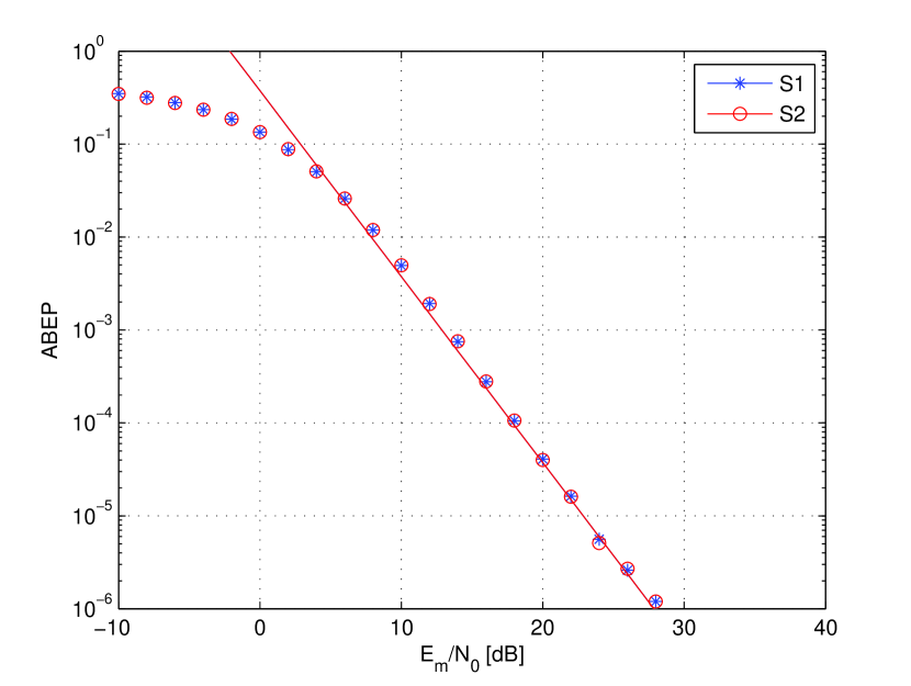
Figure 1: ABEP of a 2–source 2–relay network. Markers show Monte Carlo simulations and solid lines show the analytical framework. Setup: i) i.i.d. fading with $\sigma_{0}^{2}=1$; and ii) $b_{R_{1}}=\hat{b}_{S_{1}R_{1}}\oplus\hat{b}_{S_{2}R_{1}}$, $b_{R_{2}}=\hat{b}_{S_{1}R_{2}}\oplus\hat{b}_{S_{2}R_{2}}$. The Separation Vector is ${\rm{SV}}=\left[{{\rm{2}}{\rm{,2}}}\right]$.

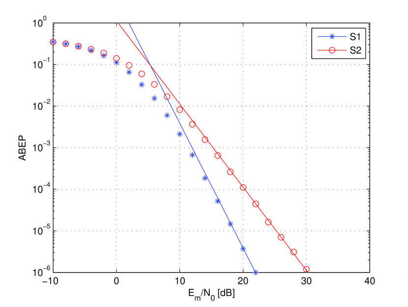
Figure 2: ABEP of a 2–source 2–relay network. Markers show Monte Carlo simulations and solid lines show the analytical framework. Setup: i) i.i.d. fading with $\sigma_{0}^{2}=1$; and ii) $b_{R_{1}}=\hat{b}_{S_{1}R_{1}}$, $b_{R_{2}}=\hat{b}_{S_{1}R_{2}}\oplus\hat{b}_{S_{2}R_{2}}$. The Separation Vector is ${\rm{SV}}=\left[{{\rm{3}}{\rm{,2}}}\right]$.

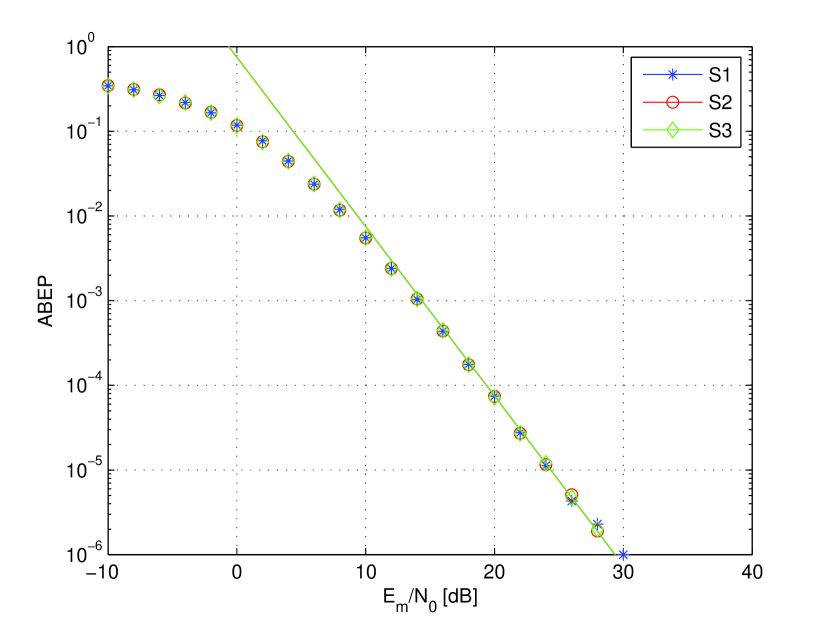
Figure 3: ABEP of a 3–source 3–relay network. Markers show Monte Carlo simulations and solid lines show the analytical framework. Setup: i) i.i.d. fading with $\sigma_{0}^{2}=1$; and ii) $b_{R_{1}}=\hat{b}_{S_{1}R_{1}}$, $b_{R_{2}}=\hat{b}_{S_{2}R_{2}}$, $b_{R_{3}}=\hat{b}_{S_{3}R_{3}}$. The Separation Vector is ${\rm{SV}}=\left[{{\rm{2}}{\rm{,2}}{\rm{,2}}}\right]$.

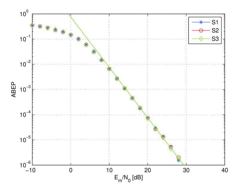
Figure 4: ABEP of a 3–source 3–relay network. Markers show Monte Carlo simulations and solid lines show the analytical framework. Setup: i) i.i.d. fading with $\sigma_{0}^{2}=1$; and ii) $b_{R_{1}}=\hat{b}_{S_{1}R_{1}}\oplus\hat{b}_{S_{2}R_{1}}\oplus\hat{b}_{S_{3}R_{1}}$, $b_{R_{2}}=\hat{b}_{S_{1}R_{2}}\oplus\hat{b}_{S_{2}R_{2}}\oplus\hat{b}_{S_{3}R_{2}}$, $b_{R_{3}}=\hat{b}_{S_{1}R_{3}}\oplus\hat{b}_{S_{2}R_{3}}\oplus\hat{b}_{S_{3}R_{3}}$. The Separation Vector is ${\rm{SV}}=\left[{{\rm{2}}{\rm{,2}}{\rm{,2}}}\right]$.

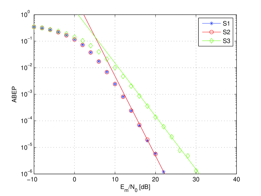
Figure 5: ABEP of a 3–source 3–relay network. Markers show Monte Carlo simulations and solid lines show the analytical framework. Setup: i) i.i.d. fading with $\sigma_{0}^{2}=1$; and ii) $b_{R_{1}}=\hat{b}_{S_{1}R_{1}}$, $b_{R_{2}}=\hat{b}_{S_{2}R_{2}}$, $b_{R_{3}}=\hat{b}_{S_{1}R_{3}}\oplus\hat{b}_{S_{2}R_{3}}\oplus\hat{b}_{S_{3}R_{3}}$. The Separation Vector is ${\rm{SV}}=\left[{{\rm{3}}{\rm{,3}}{\rm{,2}}}\right]$.

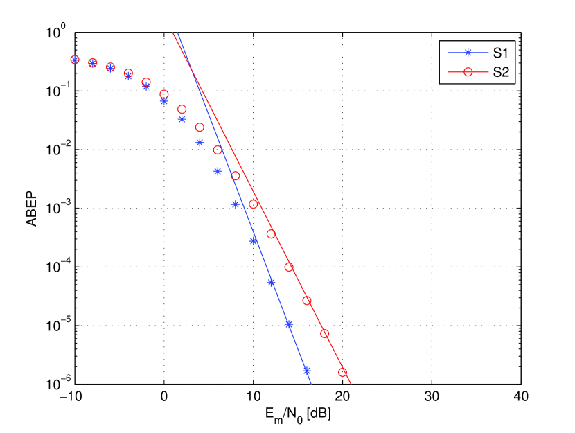
Figure 6: ABEP of a 2–source 5–relay network. Markers show Monte Carlo simulations and solid lines show the analytical framework. Setup: i) i.i.d. fading with $\sigma_{0}^{2}=1$; and ii) $b_{R_{1}}=\hat{b}_{S_{1}R_{1}}$, $b_{R_{2}}=\hat{b}_{S_{1}R_{2}}$, $b_{R_{3}}=\hat{b}_{S_{1}R_{3}}$, $\hat{b}_{R_{4}}=\hat{b}_{S_{2}R_{4}}$, $\hat{b}_{R_{5}}=\hat{b}_{S_{2}R_{5}}$. The Separation Vector is ${\rm{SV}}=\left[{{\rm{4}}{\rm{,3}}}\right]$.

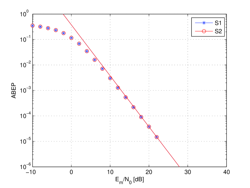
Figure 7: ABEP of a 2–source 5–relay network. Markers show Monte Carlo simulations and solid lines show the analytical framework. Setup: i) i.i.d. fading with $\sigma_{0}^{2}=1$; and ii) $b_{R_{1}}=\hat{b}_{S_{1}R_{1}}\oplus\hat{b}_{S_{2}R_{1}}$, $b_{R_{2}}=\hat{b}_{S_{1}R_{2}}\oplus\hat{b}_{S_{2}R_{2}}$, $b_{R_{3}}=\hat{b}_{S_{1}R_{3}}\oplus\hat{b}_{S_{2}R_{3}}$, $b_{R_{4}}=\hat{b}_{S_{1}R_{4}}\oplus\hat{b}_{S_{2}R_{4}}$, $b_{R_{5}}=\hat{b}_{S_{1}R_{5}}\oplus\hat{b}_{S_{2}R_{5}}$. The Separation Vector is ${\rm{SV}}=\left[{{\rm{2}}{\rm{,2}}}\right]$.

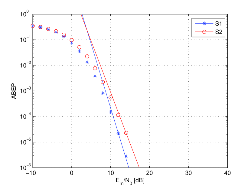
Figure 8: ABEP of a 2–source 5–relay network. Markers show Monte Carlo simulations and solid lines show the analytical framework. Setup: i) i.i.d. fading with $\sigma_{0}^{2}=1$; and ii) $b_{R_{1}}=\hat{b}_{S_{1}R_{1}}$, $b_{R_{2}}=\hat{b}_{S_{1}R_{2}}$, $b_{R_{3}}=\hat{b}_{S_{1}R_{3}}\oplus\hat{b}_{S_{2}R_{3}}$, $b_{R_{4}}=\hat{b}_{S_{1}R_{4}}\oplus\hat{b}_{S_{2}R_{4}}$, $b_{R_{5}}=\hat{b}_{S_{2}R_{5}}$. The Separation Vector is ${\rm{SV}}=\left[{{\rm{5}}{\rm{,4}}}\right]$.

Figs. 1–8 show the end–to–end ABEP for three network topologies ($N_{S}=2$ and $N_{R}=2$; $N_{S}=3$ and $N_{R}=3$; $N_{S}=2$ and $N_{R}=5$) and for different network codes. In particular, the network codes are chosen according to three criteria: i) NC is not used and only cooperation is exploited to improve the performance; ii) all the relay nodes implement binary NC on all the received data, as it is often assumed in the literature [25]; and iii) only some relay nodes perform NC on a subset of receiver packets. The first class of codes provides the reference scenario to understand the benefit of NC over classical cooperative protocols. The second class of codes represents the baseline scenario for network–coded cooperative networks. Finally, the third class of codes is important to highlight UEP capabilities, and to show that a non–negligible improvement can be obtained if the network code is properly designed and only some sources are network–coded. Numerical examples confirm the tightness of our framework for high–SNR, and that both diversity order and coding gain can be well estimated with our simple framework. Furthermore, the UEP behavior of many network codes can be observed as well. In particular, by comparing the SVs summarized in the caption of each figure with the slope of each curve, we can notice a perfect match, as predicted in Section V. Finally, we note that by comparing the results of the 2–source 2–relay network with the results of the 2–source 5–relay network, we can notice that if the network code is not properly chosen, having multiple relays does not necessarily lead to a better diversity order. Since the rate of the system is smaller for larger networks (more relays), we can conclude that small networks with well–optimized network codes can outperform large networks where the network code is not adequately chosen. What really matters to optimize the performance of multi–source multi–relay networks is the SV of the network code, and, thus, the way the packets received at the relays are mixed together.

Impact of the Source–to–Relay Links on the Achievable Performance

In Table I, we show a comparative study of the performance of three network topologies for realistic source–to–relay links, along with the scenario where ${\sigma_{S_{t}R_{q}}^{2}\to\infty}$ for $t=1,2,\ldots,N_{S}$ and $q=1,2,\ldots,N_{R}$, which is denoted as “ideal” in the table. The results have been obtained from the analytical models and have been verified through Monte Carlo simulations. The accuracy between model and simulation for the “realistic” scenario can be verified in Figs. 1–8, since the same simulation setup is used. On the other hand, due to space limitations, similar curves for the “ideal” case are not shown, but similar accuracy has been obtained. The framework used for this latter scenario is given in Corollary 4. As discussed in Section IV-C, Table I confirms that there is no diversity loss between the two scenarios, but only a coding gain loss can be expected. This is because for both scenarios the ML–optimum demodulator is used. However, the conclusions about the usefulness of NC for both scenarios can be quite different. Let us consider, for example, the 2–source 2–relay network. In the “ideal” setting, there is no doubt that NC–3 and NC–4 should be preferred to NC–1 (no NC) and to NC–2 (all received data packets are network–coded), as one user achieves a higher diversity order while the other has the same ABEP as NC–1 and NC–2. On the other hand, the conclusion in the “realistic” setting is different. In this case, we observe that the higher diversity order achieved by one user is compensated by a coding gain loss for the second user. In other words, a coding/diversity gain tradeoff exists. However, this behavior is in the spirit of cooperative networking: one user might tolerate a performance degradation in a given communication round and wait for a reward during another communication round. Properly choosing the network code enables this possibility. Furthermore, by comparing NC–1 and NC–2, we can notice that different conclusions can be drawn about the usefulness of NC in the analyzed scenarios. In the “ideal” setting, a cooperative network with NC (NC–2) has the same ABEP as a cooperative network without NC (NC–1). The conclusion is that NC is useless in this case. On the other hand, the situation changes in the “realistic” setting. In this case, we can see that NC–2 is superior to NC–1, and, thus, we conclude that the redundancy introduced by NC can be efficiently exploited at the receiver when it operates in harsh fading scenarios. In fact, in the “realistic” setting, NC–2 can counteract the error propagation due to the dual–hop protocol, even though this network code is not strong enough to achieve a higher diversity order. Another contradictory behavior can be found when analyzing the 3–source 3–relay network. By comparing NC–1 (no NC) and NC–2 (the relays apply NC to all received packets), we notice that in the “ideal” setting NC turns out to be harmful, as NC–2 provides worse performance than NC–1. On the other hand, in the “realistic” setting we notice that NC–1 and NC–2 provides the same ABEP. In other words, NC does not help but at least it is not harmful. These examples, even though specific to particular networks and codes, clearly illustrate the importance of considering realistic source–to–relay links to draw sound conclusions about merits and demerits of NC for multi–source multi–relay networks over fading channels. Furthermore, we mention that, for all the network topologies studied in Table I, NC–2 is representative of a network code that has been designed by keeping (38) in mind, as it provides the same high–SNR diversity order and coding gain for both “ideal” and “realistic” settings. Finally, we emphasize that our conclusions and trends depend on the coding gain of the network, whose study is often neglected due to its analytical intractability [16], [18], [19], [25]. In this paper, we succeeded to provide an accurate estimate of the coding gain as well.

Accuracy of the Framework for i.n.i.d. Fading Channels and Impact of Relay Positions

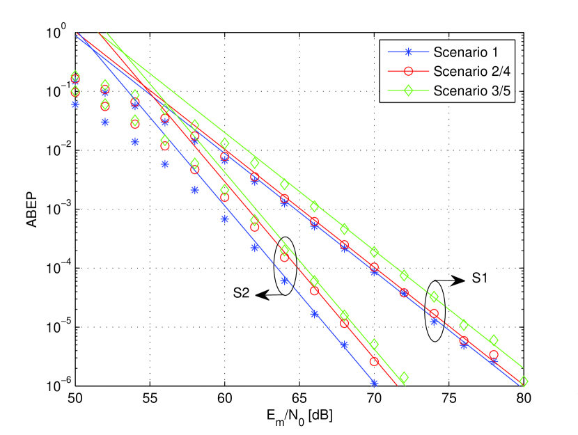
Figure 9: ABEP of a 2–source 2–relay network. Markers show Monte Carlo simulations and solid lines show the analytical framework. Setup. i) i.n.i.d. scenario with $\alpha=3$, $\sigma_{XY}^{2}=d_{XY}^{-\alpha}$, ii) the nodes are located at positions (in meters): $S_{1}=\left({0,25}\right)$, $S_{2}=\left({0,-25}\right)$, $D=\left({50,0}\right)$, $R_{1}=\left({x_{R_{1}},12.5}\right)$, $R_{2}=\left({x_{R_{2}},-12.5}\right)$; and iii) $b_{R_{1}}=\hat{b}_{S_{1}R_{1}}\oplus\hat{b}_{S_{2}R_{1}}$, $b_{R_{2}}=\hat{b}_{S_{2}R_{2}}$. Furthermore, we have: i) $x_{R_{1}}=25$ and $x_{R_{2}}=25$ in Scenario 1; ii) $x_{R_{1}}=5$ and $x_{R_{2}}=5$ in Scenario 2; iii) $x_{R_{1}}=45$ and $x_{R_{2}}=45$ in Scenario 3; iv) $x_{R_{1}}=5$ and $x_{R_{2}}=45$ in Scenario 4; v) $x_{R_{1}}=45$ and $x_{R_{2}}=5$ in Scenario 5.

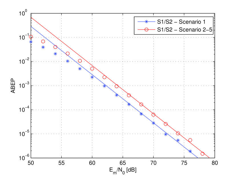
Figure 10: ABEP of a 2–source 2–relay network. Markers show Monte Carlo simulations and solid lines show the analytical framework. Setup. i) i.n.i.d. scenario with $\alpha=3$, $\sigma_{XY}^{2}=d_{XY}^{-\alpha}$, ii) the nodes are located at positions (in meters): $S_{1}=\left({0,25}\right)$, $S_{2}=\left({0,-25}\right)$, $D=\left({50,0}\right)$, $R_{1}=\left({x_{R_{1}},12.5}\right)$, $R_{2}=\left({x_{R_{2}},-12.5}\right)$; and iii) $b_{R_{1}}=\hat{b}_{S_{1}R_{1}}$, $b_{R_{2}}=\hat{b}_{S_{2}R_{2}}$. Furthermore, we have: i) $x_{R_{1}}=25$ and $x_{R_{2}}=25$ in Scenario 1; ii) $x_{R_{1}}=5$ and $x_{R_{2}}=5$ in Scenario 2; iii) $x_{R_{1}}=45$ and $x_{R_{2}}=45$ in Scenario 3; iv) $x_{R_{1}}=5$ and $x_{R_{2}}=45$ in Scenario 4; v) $x_{R_{1}}=45$ and $x_{R_{2}}=5$ in Scenario 5.

In Fig. 9 and Fig. 10, we analyze the accuracy of the framework for i.n.i.d. fading channels. We consider a 2–source 2–relay network with nodes located as described in the caption of the figures. We consider five network topologies where the relay nodes can occupy different positions with respect to source and destination nodes. We observe a good accuracy of the framework, and notice that the positions of the relays can affect the end–to–end performance. This example shows that the proposed framework can be used, for arbitrary fading parameters, for performance optimization via optimal relay placement.

Impact of Receiver CSI on the Diversity Order

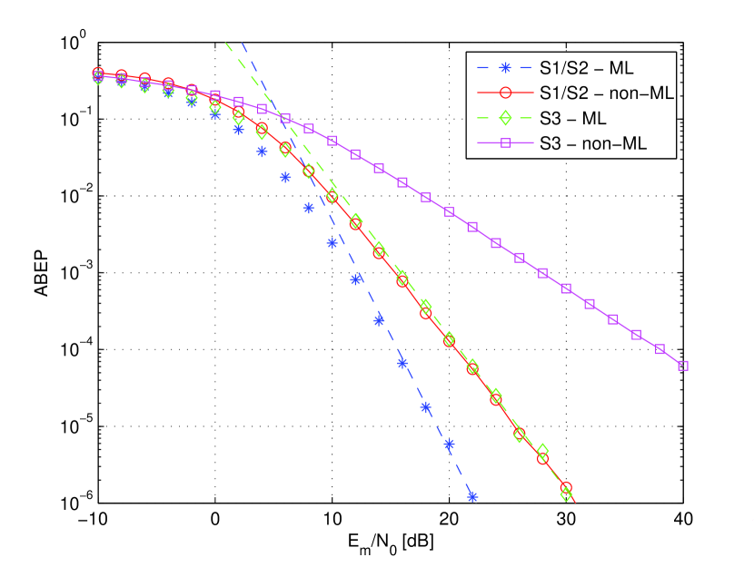
Figure 11: ABEP of a 3–source 3–relay network. Markers show Monte Carlo simulations for the ML demodulator, dashed lines show the analytical framework for the ML demodulator, and solid lines with markers show Monte Carlo simulation of the non–ML demodulator. Setup: i) i.i.d. fading with $\sigma_{0}^{2}=1$; and ii) $b_{R_{1}}=\hat{b}_{S_{1}R_{1}}$, $b_{R_{2}}=\hat{b}_{S_{2}R_{2}}$, $b_{R_{3}}=\hat{b}_{S_{1}R_{3}}\oplus\hat{b}_{S_{2}R_{3}}\oplus\hat{b}_{S_{3}R_{3}}$.

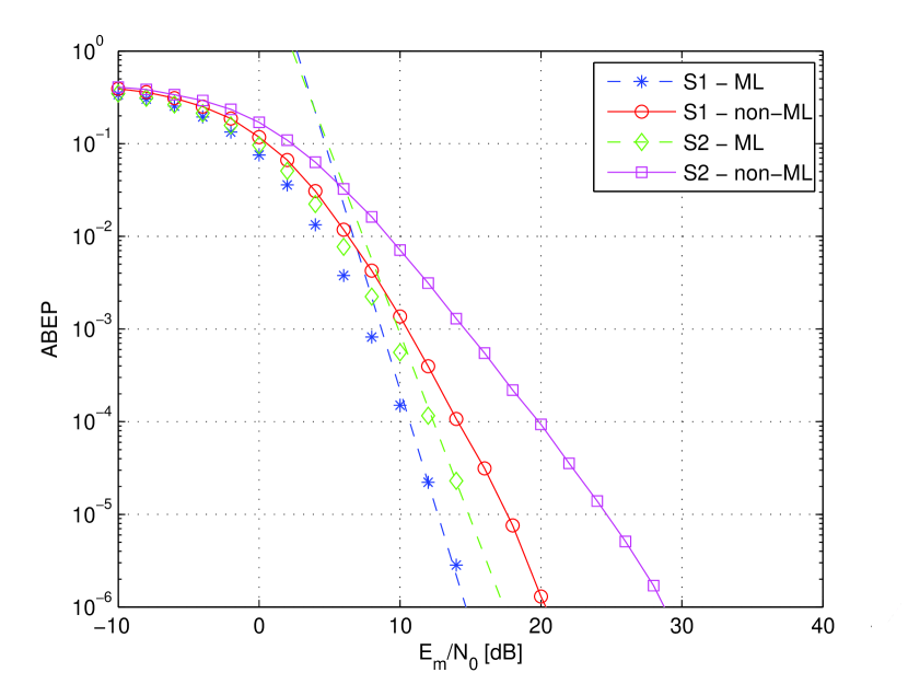
Figure 12: ABEP of a 2–source 5–relay network. Markers show Monte Carlo simulations for the ML demodulator, dashed lines show the analytical framework for the ML demodulator, and solid lines with markers show Monte Carlo simulation of the non–ML demodulator. Setup: i) i.i.d. fading with $\sigma_{0}^{2}=1$; and ii) $b_{R_{1}}=\hat{b}_{S_{1}R_{1}}$, $b_{R_{2}}=\hat{b}_{S_{1}R_{2}}$, $b_{R_{3}}=\hat{b}_{S_{1}R_{3}}\oplus\hat{b}_{S_{2}R_{3}}$, $b_{R_{4}}=\hat{b}_{S_{1}R_{4}}\oplus\hat{b}_{S_{2}R_{4}}$, $b_{R_{5}}=\hat{b}_{S_{2}R_{5}}$.

In Fig. 11 and Fig. 12, we study the impact of using the sub–optimal non–ML demodulator in (39). In particular, the ABEP of this demodulator is computed by using Monte Carlo simulations, and it is compared to the analytical investigation in Section V-B. For comparison, the ABEP (analytical framework and Monte Carlo simulations) of the ML–optimum demodulator in (6) is shown as well. The non–negligible drop of the diversity order can be observed, and, by direct inspection, it can be noticed that the curves have the slope predicted in (40). This confirms the importance of CSI about the source–to–relay links in order to avoid substantial performance degradation.

VII Conclusion

In this paper, we have proposed a new analytical framework to study the performance of multi–source multi–relay network–coded cooperative wireless networks for generic network topologies and binary encoding vectors. Our framework takes into account practical communication constraints, such as demodulation errors at the relay nodes and fading over all the wireless links. More specifically, closed–form expressions of the cross–over probability at each relay node are given, and end–to–end closed–form expressions of ABEP and diversity/coding gain are provided. Our analysis has pointed out that the achievable diversity of each source node coincides with the separation vector of the network code, which shows that NC can offer unequal diversity capabilities for different sources. Also, the importance of CSI about the source–to–relay channels has been studied, and it has been proved that half of the diversity might be lost if the reliability of the source–to–relay links is not properly taken into account at the destination. Monte Carlo simulations have been used to substantiate analytical modeling and theoretical findings for various network topologies and network codes. In particular, numerical examples have confirmed that the proposed framework is asymptotically–tight for high SNRs. Finally, by comparing the performance of various network topologies, with and without taking into account decoding errors at the relays, we have shown that wrong conclusions about the effectiveness and potential gain of NC for cooperative networks might be drawn when network operations are oversimplified. This highlights the importance of studying the performance of network–coded cooperative wireless networks with practical communication constraints for a pragmatic assessment of the end–to–end performance and to enable the efficient optimization of these networks. The framework proposed in this paper provides an answer to this problem.

Appendix A Proofs of Lemma 1, Lemma 2, and Lemma 3

A-A Proof of Lemma 1

Lemma 1

Let $T_{1}={\rm{E}}_{\bf{h}}\left\{{\prod\nolimits_{k=1}^{d_{H}\left({{\bf{c}},{\bf{\bar{c}}}}\right)}{{\bf{P}}\left[{\bar{m}_{\left({{\bf{c}},{\bf{\bar{c}}}}\right)}^{\left(k\right)}}\right]}}\right\}$, with ${\bf{P}}=\left[{P_{S_{1}D},\ldots,P_{S_{N_{S}}D},P_{S_{1:N_{S}}R_{1}D},\ldots,P_{S_{1:N_{S}}R_{N_{R}}D}}\right]^{T}$ and ${\bf{P}}\left[m\right]$, for $m=1,2,\ldots,N_{S}+N_{R}$, given in Section III and in Proposition 1. Then, over i.n.i.d. Rayleigh fading channels and for high–SNR, $T_{1}$ has closed–form expression as follows:

$$\scriptsize T_{1}\to\left({4\frac{{E_{m}}}{{N_{0}}}}\right)^{-d_{H}\left({{\bf{c}},{\bf{\bar{c}}}}\right)}\prod\limits_{m=1}^{N_{S}+N_{R}}{\chi\left\{{{\bf{\Delta}}_{{\bf{c}},{\bf{\bar{c}}}}\left[m\right]{\bf{\bar{\Sigma}}}_{{\rm{SRD}}}^{\left({\bf{G}}\right)}\left[m\right]}\right\}}$$ (42)

where all symbols are defined in Proposition 3.

Proof: Owing to the assumption of independent fading channels, it follows, by direct inspection, that ${\bf{P}}\left[m\right]$ for $m=1,2,\ldots,N_{S}+N_{R}$ are independent RVs, and, thus, $T_{1}=\prod\nolimits_{k=1}^{d_{H}\left({{\bf{c}},{\bf{\bar{c}}}}\right)}{{\rm{E}}_{\bf{h}}\left\{{{\bf{P}}\left[{\bar{m}_{\left({{\bf{c}},{\bf{\bar{c}}}}\right)}^{\left(k\right)}}\right]}\right\}}=\prod\nolimits_{k=1}^{d_{H}\left({{\bf{c}},{\bf{\bar{c}}}}\right)}{{\bf{\bar{P}}}\left[{\bar{m}_{\left({{\bf{c}},{\bf{\bar{c}}}}\right)}^{\left(k\right)}}\right]}$, where ${\bf{\bar{P}}}\left[{\bar{m}_{\left({{\bf{c}},{\bf{\bar{c}}}}\right)}^{\left(k\right)}}\right]={\rm{E}}_{\bf{h}}\left\{{{\bf{P}}\left[{\bar{m}_{\left({{\bf{c}},{\bf{\bar{c}}}}\right)}^{\left(k\right)}}\right]}\right\}$. Furthermore, from the definition of ${\bf{P}}\left[m\right]$ in Section III and Proposition 1, for high–SNR we have:

$$\scriptsize\bar{P}_{S_{t}D}\to\left({4\frac{{E_{m}}}{{N_{0}}}\sigma_{S_{t}D}^{2}}\right)^{-1}\quad{\rm{and}}\quad\bar{P}_{S_{1:N_{S}}R_{q}D}\to\sum\limits_{t=1}^{N_{S}}{\left[{g_{S_{t}R_{q}}\left({4\frac{{E_{m}}}{{N_{0}}}\sigma_{S_{t}R_{q}}^{2}}\right)^{-1}}\right]}+\left({4\frac{{E_{m}}}{{N_{0}}}\sigma_{R_{q}D}^{2}}\right)^{-1}$$ (43)

The results in (43) can be obtained from the following chain of equalities and high–SNR approximations:

$$\scriptsize\left\{\begin{array}[]{l}\bar{P}_{XY}={\rm{E}}_{\bf{h}}\left\{{Q\left({\sqrt{2\left({{{E_{m}}\mathord{\left/{\vphantom{{E_{m}}{N_{0}}}}\right.\kern-1.2pt}{N_{0}}}}\right)\left|{h_{XY}}\right|^{2}}}\right)}\right\}\mathop{=}\limits^{\left({a_{1}}\right)}\frac{1}{2}\left[{1-\sqrt{\frac{{\left({{{E_{m}}\mathord{\left/{\vphantom{{E_{m}}{N_{0}}}}\right.\kern-1.2pt}{N_{0}}}}\right)\sigma_{XY}^{2}}}{{1+\left({{{E_{m}}\mathord{\left/{\vphantom{{E_{m}}{N_{0}}}}\right.\kern-1.2pt}{N_{0}}}}\right)\sigma_{XY}^{2}}}}}\right]\mathop{\to}\limits^{\left({a_{2}}\right)}\left({4\frac{{E_{m}}}{{N_{0}}}\sigma_{XY}^{2}}\right)^{-1}\\ \bar{P}_{S_{1:N_{S}}R_{q}D}={\rm{E}}_{\bf{h}}\left\{{P_{S_{1:N_{S}}R_{q}}+P_{R_{q}D}-2P_{S_{1:N_{S}}R_{q}}P_{R_{q}D}}\right\}\mathop{=}\limits^{\left({b_{1}}\right)}\bar{P}_{S_{1:N_{S}}R_{q}}+\bar{P}_{R_{q}D}-2\bar{P}_{S_{1:N_{S}}R_{q}}\bar{P}_{R_{q}D}\mathop{\to}\limits^{\left({b_{2}}\right)}\bar{P}_{S_{1:N_{S}}R_{q}}+\bar{P}_{R_{q}D}\\ \bar{P}_{S_{1:N_{S}}R_{q}}=\sum\limits_{t=1}^{N_{S}}{\left[{g_{S_{t}R_{q}}\bar{P}_{S_{t}R_{q}}\prod\limits_{r=t+1}^{N_{S}}{\left({1-2g_{S_{r}R_{q}}\bar{P}_{S_{r}R_{q}}}\right)}}\right]}\mathop{\to}\limits^{\left({c_{1}}\right)}\sum\limits_{t=1}^{N_{S}}{g_{S_{t}R_{q}}\bar{P}_{S_{t}R_{q}}}\mathop{\to}\limits^{\left({c_{2}}\right)}\sum\limits_{t=1}^{N_{S}}{\left[{g_{S_{t}R_{q}}\left({4\frac{{E_{m}}}{{N_{0}}}\sigma_{S_{t}R_{q}}^{2}}\right)^{-1}}\right]}\\ \end{array}\right.$$ (44)

where: i) $\mathop{=}\limits^{\left({a_{1}}\right)}$ comes from [52, Eq. (14–3–7)]; ii) $\mathop{\to}\limits^{\left({a_{2}}\right)}$ is the high–SNR approximation of $\mathop{=}\limits^{\left({a_{1}}\right)}$ in [52, Eq. (14–3–13)]; iii) $\mathop{\to}\limits^{\left({b_{2}}\right)}$ is the high–SNR approximation of $\mathop{=}\limits^{\left({b_{1}}\right)}$, which simply neglects the term $\bar{P}_{S_{1:N_{S}}R_{q}}\bar{P}_{R_{q}D}$, as it decays faster for high–SNR; iv) $\mathop{\to}\limits^{\left({c_{1}}\right)}$ follows by noticing that $1-2g_{S_{r}R_{q}}\bar{P}_{S_{r}R_{q}}\to 1$ for high–SNR; and v) $\mathop{\to}\limits^{\left({c_{2}}\right)}$ is, similar to $\mathop{\to}\limits^{\left({a_{2}}\right)}$, is the high–SNR approximation of $\mathop{\to}\limits^{\left({c_{1}}\right)}$. From (44), (42) follows by using notation and vector representation in Proposition 3. More specifically, the vector ${{\bf{\Delta}}_{{\bf{c}},{\bf{\bar{c}}}}}$ takes into account that only the indexes in the set $\Theta\left({{\bf{c}},{\bf{\bar{c}}}}\right)=\left\{{m|{\bf{c}}\left[m\right]\neq{\bf{\bar{c}}}\left[m\right]}\right\}$ have to be included in $T_{1}$, and the vector ${{\bf{\bar{\Sigma}}}_{{\rm{SRD}}}^{\left({\bf{G}}\right)}}$ accounts for the dual–hop relaying protocol and the specific network code. This concludes the proof. $\Box$

Two important remarks are worth being made about Lemma 1. First, we would like to emphasize that, for ease of presentation and to stay focused on the most important issues of our analysis, i.e., dual–hop networking and NC, the results in (42) and (43) are here given for Rayleigh fading only. However, they can be generalized to other fading distributions for which the high–SNR approximation in [61] exists. In this paper, Rayleigh fading is studied for illustrative purposes only. Second, by comparing $\mathop{\to}\limits^{\left({c_{2}}\right)}$ and [62, Eq. (40)], it follows that, for high–SNR, the effect, on the error probability at the relays, of performing NC on noisy and faded received data is equivalent to an Amplify–and–Forward (AF) relay protocol with CSI–assisted relaying [60] and with a number of hops equal to the number of sources that are network–coded at each relay. This conclusion is in agreement with the equivalence between the error probability at the relays and the error performance of DemF relay protocols already highlighted in Section III-A. In fact, in [58] it has been shown that, except when the number of hops is very large and the fading severity is very small, the performance of AF and DemF protocols is very close, for high–SNR, to each other. As the number of sources that can be network–coded is, for practical applications, not very large, this high–SNR approximation can be very useful to get formulas that provide insights on the system behavior. The high–SNR equivalency between (43) and AF relaying is exploited in Lemma 2 to get high–SNR but closed–form and accurate formulas.

A-B Proof of Lemma 2

Lemma 2

Let us consider the term $T_{2}={\rm{E}}_{\bf{h}}\left\{{\min\left\{{\prod\nolimits_{k\in{\rm\mathcal{A}}}{{\bf{P}}\left[{\bar{m}_{\left({{\bf{c}},{\bf{\bar{c}}}}\right)}^{\left(k\right)}}\right]},\prod\nolimits_{k\in\bar{\rm\mathcal{A}}}{{\bf{P}}\left[{\bar{m}_{\left({{\bf{c}},{\bf{\bar{c}}}}\right)}^{\left(k\right)}}\right]}}\right\}}\right\}$, with ${\bf{P}}=\left[{P_{S_{1}D},\ldots,P_{S_{N_{S}}D},P_{S_{1:N_{S}}R_{1}D},\ldots,P_{S_{1:N_{S}}R_{N_{R}}D}}\right]^{T}$ and ${\bf{P}}\left[m\right]$ for $m=1,2,\ldots,N_{S}+N_{R}$ given in Section III and in Proposition 1. Then, over i.n.i.d. Rayleigh fading and for high–SNR, $T_{2}$ has closed–form expression:

$$\scriptsize T_{2}\to\left({4\frac{{E_{m}}}{{N_{0}}}}\right)^{-d_{H}\left({{\bf{c}},{\bf{\bar{c}}}}\right)}\left[{\frac{{2\sqrt{\pi}\Gamma\left({d_{H}\left({{\bf{c}},{\bf{\bar{c}}}}\right)+\frac{1}{2}}\right)}}{{\Gamma\left({d+\frac{1}{2}}\right)\Gamma\left({d_{H}\left({{\bf{c}},{\bf{\bar{c}}}}\right)-d+\frac{1}{2}}\right)}}}\right]\prod\limits_{m=1}^{N_{S}+N_{R}}{\chi\left\{{{\bf{\Delta}}_{{\bf{c}},{\bf{\bar{c}}}}\left[m\right]{\bf{\bar{\Sigma}}}_{{\rm{SRD}}}^{\left({\bf{G}}\right)}\left[m\right]}\right\}}$$ (45)

where all symbols are defined in Proposition 3.

Proof: The computation of $T_{2}$ is very analytically involving. To get accurate, but closed–form and insightful formulas that can shed lights on the network behavior, we exploit some high–SNR approximations. More specifically, the starting point is the following high–SNR approximation:

$$\scriptsize\left\{\begin{array}[]{l}P_{S_{t}D}=Q\left({\sqrt{2\left({{{E_{m}}\mathord{\left/{\vphantom{{E_{m}}{N_{0}}}}\right.\kern-1.2pt}{N_{0}}}}\right)\left|{h_{S_{t}D}}\right|^{2}}}\right)\\ P_{S_{1:N_{S}}R_{q}D}=P_{S_{1:N_{S}}R_{q}}+P_{R_{q}D}-2P_{S_{1:N_{S}}R_{q}}P_{R_{q}D}\mathop{\to}\limits^{\left(a\right)}Q\left({\sqrt{2\left({{{E_{m}}\mathord{\left/{\vphantom{{E_{m}}{N_{0}}}}\right.\kern-1.2pt}{N_{0}}}}\right)\left[{\left|{h_{R_{q}D}}\right|^{-2}+\sum\limits_{t=1}^{N_{S}}{g_{S_{t}R_{q}}\left|{h_{S_{t}R_{q}}}\right|^{-2}}}\right]^{-1}}}\right)\\ \end{array}\right.$$ (46)

The approximation in $\mathop{\to}\limits^{\left(a\right)}$ follows from the closing comment in Lemma 1, where we have proved that for high–SNR the cumulative error due to performing NC on wrong demodulated bits at the relays can be well–approximated by an equivalent AF multi–hop relay network with a number of hops that is equal to the number of network–coded sources. In particular, from [60] we can recognize that the argument of the Q–function in $\mathop{\to}\limits^{\left(a\right)}$ is the end–to–end SNR of an AF relay network, which takes into account the relay–to–destination link and the cumulative error due to combining, at the most, $N_{S}$ source. The number of sources that are actually network–coded depends on the number of non–zero NC coefficients ${g_{S_{t}R_{q}}}$. Let us emphasize that the formula for the direct source–to–destination link is exact, but we have decided to re–write it to better understand that high–SNR approximation applies only to the signals forwarded from the relays. Thus, in $T_{2}$, we have ${\bf{P}}\left[{\bar{m}_{\left({{\bf{c}},{\bf{\bar{c}}}}\right)}^{\left(k\right)}}\right]\to Q\left({\sqrt{2\left({{{E_{m}}\mathord{\left/{\vphantom{{E_{m}}{N_{0}}}}\right.\kern-1.2pt}{N_{0}}}}\right){\rm{SNR}}_{\left({{\bf{c}},{\bf{\bar{c}}}}\right)}^{\left(k\right)}}}\right)$, where: i) ${\rm{SNR}}_{\left({{\bf{c}},{\bf{\bar{c}}}}\right)}^{\left(k\right)}=\left|{h_{S_{t}D}}\right|^{2}$ for the source–to–destination links, and by bearing in mind that in this case we have a true equality; and ii) ${\rm{SNR}}_{\left({{\bf{c}},{\bf{\bar{c}}}}\right)}^{\left(k\right)}=\left[{\left|{h_{R_{q}D}}\right|^{-2}+\sum\nolimits_{t=1}^{N_{S}}{g_{S_{t}R_{q}}\left|{h_{S_{t}R_{q}}}\right|^{-2}}}\right]^{-1}$ for the relay–to–destination links. Thus, $T_{2}$ simplifies:

$$\scriptsize\begin{split}T_{2}&\to{\rm{E}}_{\bf{h}}\left\{{\min\left\{{\prod\limits_{k\in{\rm\mathcal{A}}}{Q\left({\sqrt{2\left({{{E_{m}}\mathord{\left/{\vphantom{{E_{m}}{N_{0}}}}\right.\kern-1.2pt}{N_{0}}}}\right){\rm{SNR}}_{\left({{\bf{c}},{\bf{\bar{c}}}}\right)}^{\left(k\right)}}}\right)},\prod\limits_{k\in\bar{\rm\mathcal{A}}}{Q\left({\sqrt{2\left({{{E_{m}}\mathord{\left/{\vphantom{{E_{m}}{N_{0}}}}\right.\kern-1.2pt}{N_{0}}}}\right){\rm{SNR}}_{\left({{\bf{c}},{\bf{\bar{c}}}}\right)}^{\left(k\right)}}}\right)}}\right\}}\right\}\\ &\mathop{\to}\limits^{\left(a\right)}{\rm{E}}_{\bf{h}}\left\{{\min\left\{{Q\left({\sqrt{2\left({{{E_{m}}\mathord{\left/{\vphantom{{E_{m}}{N_{0}}}}\right.\kern-1.2pt}{N_{0}}}}\right)\Upsilon_{1}\sum\limits_{k\in{\rm\mathcal{A}}}{{\rm{SNR}}_{\left({{\bf{c}},{\bf{\bar{c}}}}\right)}^{\left(k\right)}}}}\right),Q\left({\sqrt{2\left({{{E_{m}}\mathord{\left/{\vphantom{{E_{m}}{N_{0}}}}\right.\kern-1.2pt}{N_{0}}}}\right)\Upsilon_{2}\sum\limits_{k\in\bar{\rm\mathcal{A}}}{{\rm{SNR}}_{\left({{\bf{c}},{\bf{\bar{c}}}}\right)}^{\left(k\right)}}}}\right)}\right\}}\right\}\\ &\mathop{=}\limits^{\left(b\right)}{\rm{E}}_{\bf{h}}\left\{{Q\left({\sqrt{2\left({{{E_{m}}\mathord{\left/{\vphantom{{E_{m}}{N_{0}}}}\right.\kern-1.2pt}{N_{0}}}}\right)\max\left\{{\Upsilon_{1}\sum\limits_{k\in{\rm\mathcal{A}}}{{\rm{SNR}}_{\left({{\bf{c}},{\bf{\bar{c}}}}\right)}^{\left(k\right)}},\Upsilon_{2}\sum\limits_{k\in\bar{\rm\mathcal{A}}}{{\rm{SNR}}_{\left({{\bf{c}},{\bf{\bar{c}}}}\right)}^{\left(k\right)}}}\right\}}}\right)}\right\}\\ \end{split}$$ (47)

where: i) the approximation in $\mathop{\to}\limits^{\left(a\right)}$ is proved in Lemma 3; ii) ${\Upsilon_{1}}$ and ${\Upsilon_{2}}$ are two constant factors whose closed–form expression is given in Lemma 3; and iii) the equality in $\mathop{=}\limits^{\left(b\right)}$ comes from the fact that the Q–function is monotonically decreasing for increasing values of its argument.

The last expression in (47) has a convenient structure that can be averaged over fading channel statistics. To this end, the following considerations can be made: i) $T_{2}$ can be seen as the ABEP of a dual–branch Selection Combining (SC) scheme, where the equivalent SNR of first and second branch is [53] ${\rm{SNR}}_{1}=2\left({{{E_{m}}\mathord{\left/{\vphantom{{E_{m}}{N_{0}}}}\right.\kern-1.2pt}{N_{0}}}}\right)\Upsilon_{1}\sum\nolimits_{k\in{\rm\mathcal{A}}}{{\rm{SNR}}_{\left({{\bf{c}},{\bf{\bar{c}}}}\right)}^{\left(k\right)}}$ and ${\rm{SNR}}_{2}=2\left({{{E_{m}}\mathord{\left/{\vphantom{{E_{m}}{N_{0}}}}\right.\kern-1.2pt}{N_{0}}}}\right)\Upsilon_{2}\sum\nolimits_{k\in\bar{\rm\mathcal{A}}}{{\rm{SNR}}_{\left({{\bf{c}},{\bf{\bar{c}}}}\right)}^{\left(k\right)}}$, respectively; ii) both ${\rm{SNR}}_{1}$ and ${\rm{SNR}}_{2}$ can be seen as the equivalent SNR of a Maximum Ratio Combining (MRC) scheme with a number of branches given by ${\rm{card}}\left\{\mathcal{A}\right\}=d$ and ${\rm{card}}\left\{{\mathcal{\bar{A}}}\right\}=d_{H}\left({{\bf{c}},{\bf{\bar{c}}}}\right)-d$, respectively; and iii) the “virtual” SC and MRC branches contain independent RVs, as it can be verified via direct inspection. Thus, a closed–form and high–SNR approximation of $T_{2}$ in (47) can be obtained by using the method in [61]. More specifically, by considering: i) the definition of ${\rm{SNR}}_{\left({{\bf{c}},{\bf{\bar{c}}}}\right)}^{\left(k\right)}$ in (47); ii) the closed–form expressions of ${\Upsilon_{1}}$ and ${\Upsilon_{2}}$ in Lemma 3; and iii) the general parametrization in [61, Prop. 1, Prop. 4] for systems with receive–diversity, we can obtain, after lengthly algebraic manipulations, the final result shown in (45). In particular, ${{\bf{\Delta}}_{{\bf{c}},{\bf{\bar{c}}}}}$ and ${{\bf{\bar{\Sigma}}}_{{\rm{SRD}}}^{\left({\bf{G}}\right)}}$ have the same meaning as in Lemma 1, while the term into the square brackets accounts for the SC/MRC high–SNR approximation of $\mathop{=}\limits^{\left(b\right)}$ in (47). This concludes the proof. $\Box$

Finally, similar to Lemma 1 we emphasize once again that the closed–form solution in (45) can be generalized to other fading channel models by using [61] and [62].

A-C Proof of Lemma 3

Lemma 3

Let $\lambda=\prod\nolimits_{k\in{\rm\mathcal{A}}}{Q\left({\sqrt{2\left({{{E_{m}}\mathord{\left/{\vphantom{{E_{m}}{N_{0}}}}\right.\kern-1.2pt}{N_{0}}}}\right){\rm{SNR}}_{\left({{\bf{c}},{\bf{\bar{c}}}}\right)}^{\left(k\right)}}}\right)}$ with ${{\rm{SNR}}_{\left({{\bf{c}},{\bf{\bar{c}}}}\right)}^{\left(k\right)}}$ defined in Lemma 2. Then, for high–SNR and Rayleigh fading, $\lambda$ can be tightly approximated as follows:

$$\scriptsize\lambda=\prod\limits_{k\in{\rm\mathcal{A}}}{Q\left({\sqrt{2\left({{{E_{m}}\mathord{\left/{\vphantom{{E_{m}}{N_{0}}}}\right.\kern-1.2pt}{N_{0}}}}\right){\rm{SNR}}_{\left({{\bf{c}},{\bf{\bar{c}}}}\right)}^{\left(k\right)}}}\right)}\to Q\left({\sqrt{2\left({{{E_{m}}\mathord{\left/{\vphantom{{E_{m}}{N_{0}}}}\right.\kern-1.2pt}{N_{0}}}}\right)\Upsilon\sum\limits_{k\in{\rm\mathcal{A}}}{{\rm{SNR}}_{\left({{\bf{c}},{\bf{\bar{c}}}}\right)}^{\left(k\right)}}}}\right)$$ (48)

where $\Upsilon=\left[{\frac{{2^{d-1}\pi^{\frac{{d-1}}{2}}\Gamma\left({d+\frac{1}{2}}\right)}}{{\Gamma\left({\frac{3}{2}}\right)^{d}\Gamma\left({d+1}\right)}}}\right]^{{1\mathord{\left/{\vphantom{1d}}\right.\kern-1.2pt}d}}$ and $d={\rm{card}}\left\{\mathcal{A}\right\}$.

Proof: From the Chernoff bound, i.e., $Q\left(x\right)\leq\left({{1\mathord{\left/{\vphantom{12}}\right.\kern-1.2pt}2}}\right)\exp\left({-{{x^{2}}\mathord{\left/{\vphantom{{x^{2}}2}}\right.\kern-1.2pt}2}}\right)\leq\exp\left({-{{x^{2}}\mathord{\left/{\vphantom{{x^{2}}2}}\right.\kern-1.2pt}2}}\right)$, which is accurate for $x\gg 1$ that in our case implies high–SNR (${{E_{m}}\mathord{\left/{\vphantom{{E_{m}}{N_{0}}}}\right.\kern-1.2pt}{N_{0}}}\gg 1$), the following approximation holds:

$$\scriptsize\prod\limits_{k\in{\rm\mathcal{A}}}{Q\left({\sqrt{x_{k}}}\right)}\to Q\left({\sqrt{\Upsilon\sum\limits_{k\in{\rm\mathcal{A}}}{x_{k}}}}\right)$$ (49)

where $\Upsilon$ is a constant correction term, which is introduced to recover the coding gain inaccuracy that might arise when using the Chernoff bound [16]. The high–SNR approximation in (49) can be explained as follows. By direct inspection, left– and right–hand side terms can be shown to have both diversity order equal to $d={\rm{card}}\left\{\mathcal{A}\right\}$. In fact, the left–hand side is the product of $d$ terms each one having diversity one. On the other hand, the right–hand side term is the error probability of a MRC scheme [53] with $d$ diversity branches at the receiver, which is known to have diversity $d$ [61]. The constant (correction) factor $\Upsilon$ is introduced only to avoid coding gain inaccuracies, which are always present when using the Chernoff bound. Since the goal of this paper is to accurately estimate both coding gain and diversity order, the accurate evaluation of $\Upsilon$ is instrumental to estimate the end–to–end performance of the system.

To get an accurate, but simple and useful for further analysis, approximation we use first–order moment matching to estimate $\Upsilon$ in (49). The motivation is that, as we will better substantiate at the end of this proof, it allows us to have a closed–form estimate of $\Upsilon$ that depends only on $d$ in (48), while it is independent of the fading parameters. In formulas, we seek to find $\Upsilon$ such that the following equality is satisfied:

$$\scriptsize{\rm{E}}_{\bf{h}}\left\{{\prod\limits_{k\in{\rm\mathcal{A}}}{Q\left({\sqrt{2\left({{{E_{m}}\mathord{\left/{\vphantom{{E_{m}}{N_{0}}}}\right.\kern-1.2pt}{N_{0}}}}\right){\rm{SNR}}_{\left({{\bf{c}},{\bf{\bar{c}}}}\right)}^{\left(k\right)}}}\right)}}\right\}={\rm{E}}_{\bf{h}}\left\{{Q\left({\sqrt{2\left({{{E_{m}}\mathord{\left/{\vphantom{{E_{m}}{N_{0}}}}\right.\kern-1.2pt}{N_{0}}}}\right)\Upsilon\sum\limits_{k\in{\rm\mathcal{A}}}{{\rm{SNR}}_{\left({{\bf{c}},{\bf{\bar{c}}}}\right)}^{\left(k\right)}}}}\right)}\right\}$$ (50)

To this end, we need closed–form expressions of both averages in (50). Once again, we use the high–SNR parametrization in [61], which leads to the following result:

$$\scriptsize\left\{\begin{array}[]{l}{\rm{E}}_{\bf{h}}\left\{{\prod\limits_{k\in{\rm\mathcal{A}}}{Q\left({\sqrt{2\left({{{E_{m}}\mathord{\left/{\vphantom{{E_{m}}{N_{0}}}}\right.\kern-1.2pt}{N_{0}}}}\right){\rm{SNR}}_{\left({{\bf{c}},{\bf{\bar{c}}}}\right)}^{\left(k\right)}}}\right)}}\right\}\mathop{\to}\limits^{\left(a\right)}\left({4\frac{{E_{m}}}{{N_{0}}}}\right)^{-d}\prod\limits_{k\in{\rm\mathcal{A}}}{\left[{\frac{1}{{\sigma_{R_{q}D}^{2}}}+\sum\limits_{t=1}^{N_{S}}{\frac{{g_{S_{t}R_{q}}}}{{\sigma_{S_{t}R_{q}}^{2}}}}}\right]}\\ {\rm{E}}_{\bf{h}}\left\{{Q\left({\sqrt{2\left({{{E_{m}}\mathord{\left/{\vphantom{{E_{m}}{N_{0}}}}\right.\kern-1.2pt}{N_{0}}}}\right)\Upsilon\sum\limits_{k\in{\rm\mathcal{A}}}{{\rm{SNR}}_{\left({{\bf{c}},{\bf{\bar{c}}}}\right)}^{\left(k\right)}}}}\right)}\right\}\mathop{\to}\limits^{\left(b\right)}\left({4\frac{{E_{m}}}{{N_{0}}}\Upsilon}\right)^{-d}\left[{\frac{{2^{d-1}\pi^{\frac{{d-1}}{2}}\Gamma\left({d+\frac{1}{2}}\right)}}{{\Gamma\left({\frac{3}{2}}\right)^{d}\Gamma\left({d+1}\right)\prod\limits_{k\in{\rm\mathcal{A}}}{\left[{\left({\frac{1}{{\sigma_{R_{q}D}^{2}}}+\sum\limits_{t=1}^{N_{S}}{\frac{{g_{S_{t}R_{q}}}}{{\sigma_{S_{t}R_{q}}^{2}}}}}\right)^{-1}}\right]}}}}\right]\\ \end{array}\right.$$ (51)

where: 1) $\mathop{\to}\limits^{\left(a\right)}$ is obtained by taking into account that (i) ${{\rm{SNR}}_{\left({{\bf{c}},{\bf{\bar{c}}}}\right)}^{\left(k\right)}}$ are statistically independent for $k\in{\rm\mathcal{A}}$; (ii) according to Lemma 2, ${{\rm{SNR}}_{\left({{\bf{c}},{\bf{\bar{c}}}}\right)}^{\left(k\right)}}$ can be seen as the end–to–end SNRs of an equivalent multi–hop AF relay protocol; and (iii) by using asymptotic analysis for multi–hop AF relay networks in [62]; and 2) $\mathop{\to}\limits^{\left(b\right)}$ is obtained from [61] and [62] by recognizing that we have to compute the average of an equivalent MRC scheme where each branch is an equivalent multi–hop network that uses the AF relay protocol. Finally, by equating the two terms in (51), $\Upsilon$ in (48) can be obtained. As mentioned above, $\Upsilon$ is independent of channel statistics. Similar to Lemma 1 and Lemma 2 we mention that the proposed procedure can be applied to any fading channel model, for which the parametrization in [61] is available. This concludes the proof. $\Box$

TABLE I: ${\rm{ABEP}}_{S_{t}}=\left({G_{c}^{\left({S_{t}}\right)}\bar{\gamma}_{m}}\right)^{-G_{d}^{\left({S_{t}}\right)}}$, where ${G_{d}^{\left({S_{t}}\right)}}$ is the diversity order, ${G_{c}^{\left({S_{t}}\right)}}$ is the coding gain, and we have defined $\gamma_{m}={E_{m}/N_{0}}$. 2–source, 2–relay network. NC–1: $b_{R_{1}}=\hat{b}_{S_{1}R_{1}}$, $b_{R_{2}}=\hat{b}_{S_{2}R_{2}}$; NC–2: $b_{R_{1}}=\hat{b}_{S_{1}R_{1}}\oplus\hat{b}_{S_{2}R_{1}}$, $b_{R_{2}}=\hat{b}_{S_{1}R_{2}}\oplus\hat{b}_{S_{2}R_{2}}$; NC–3: $b_{R_{1}}=\hat{b}_{S_{1}R_{1}}\oplus\hat{b}_{S_{2}R_{1}}$, $b_{R_{2}}=\hat{b}_{S_{2}R_{2}}$; NC–4: $b_{R_{1}}=\hat{b}_{S_{1}R_{1}}$, $b_{R_{2}}=\hat{b}_{S_{1}R_{2}}\oplus\hat{b}_{S_{2}R_{2}}$. 3–source, 3–relay network. NC–1: $b_{R_{1}}=\hat{b}_{S_{1}R_{1}}$, $b_{R_{2}}=\hat{b}_{S_{2}R_{2}}$, $b_{R_{3}}=\hat{b}_{S_{3}R_{3}}$; NC–2: $b_{R_{1}}=\hat{b}_{S_{1}R_{1}}\oplus\hat{b}_{S_{2}R_{1}}\oplus\hat{b}_{S_{3}R_{1}}$, $b_{R_{2}}=\hat{b}_{S_{1}R_{2}}\oplus\hat{b}_{S_{2}R_{2}}\oplus\hat{b}_{S_{3}R_{2}}$, $b_{R_{3}}=\hat{b}_{S_{1}R_{3}}\oplus\hat{b}_{S_{2}R_{3}}\oplus\hat{b}_{S_{3}R_{3}}$; NC–3: $b_{R_{1}}=\hat{b}_{S_{1}R_{1}}$, $b_{R_{2}}=\hat{b}_{S_{2}R_{2}}$, $b_{R_{3}}=\hat{b}_{S_{1}R_{3}}\oplus\hat{b}_{S_{2}R_{3}}\oplus\hat{b}_{S_{3}R_{3}}$. 2–source, 5–relay network. NC–1: $b_{R_{1}}=\hat{b}_{S_{1}R_{1}}$, $b_{R_{2}}=\hat{b}_{S_{1}R_{2}}$, $b_{R_{3}}=\hat{b}_{S_{1}R_{3}}$, $b_{R_{4}}=\hat{b}_{S_{2}R_{4}}$, $b_{R_{4}}=\hat{b}_{S_{2}R_{5}}$; NC–2: $b_{R_{1}}=\hat{b}_{S_{1}R_{1}}\oplus\hat{b}_{S_{2}R_{1}}$, $b_{R_{2}}=\hat{b}_{S_{1}R_{2}}\oplus\hat{b}_{S_{2}R_{2}}$, $b_{R_{3}}=\hat{b}_{S_{1}R_{3}}\oplus\hat{b}_{S_{2}R_{3}}$, $b_{R_{4}}=\hat{b}_{S_{1}R_{4}}\oplus\hat{b}_{S_{2}R_{4}}$, $b_{R_{5}}=\hat{b}_{S_{1}R_{5}}\oplus\hat{b}_{S_{2}R_{5}}$; NC–3: $b_{R_{1}}=\hat{b}_{S_{1}R_{1}}$, $b_{R_{2}}=\hat{b}_{S_{1}R_{2}}$, $b_{R_{3}}=\hat{b}_{S_{1}R_{3}}\oplus\hat{b}_{S_{2}R_{3}}$, $b_{R_{4}}=\hat{b}_{S_{1}R_{4}}\oplus\hat{b}_{S_{2}R_{4}}$, $b_{R_{5}}=\hat{b}_{S_{2}R_{5}}$. Finally, i.i.d. fading with $\sigma_{0}^{2}=1$ is considered.

Network: 2–source, 2–relay
	Ideal source–to–relay channels			Realistic source–to–relay channels
	${\rm{ABEP}}_{\infty}^{\left({S_{1}}\right)}$	${\rm{ABEP}}_{\infty}^{\left({S_{2}}\right)}$	${\rm{ABEP}}_{\infty}^{\left({S_{3}}\right)}$	${\rm{ABEP}}_{\infty}^{\left({S_{1}}\right)}$	${\rm{ABEP}}_{\infty}^{\left({S_{2}}\right)}$	${\rm{ABEP}}_{\infty}^{\left({S_{3}}\right)}$
NC-1	$0.3750\gamma_{m}^{-2}$	$0.3750\gamma_{m}^{-2}$	-	$0.7500\gamma_{m}^{-2}$	$0.7500\gamma_{m}^{-2}$	-
NC-2	$0.3750\gamma_{m}^{-2}$	$0.3750\gamma_{m}^{-2}$	-	$0.3750\gamma_{m}^{-2}$	$0.3750\gamma_{m}^{-2}$	-
NC-3	$0.3750\gamma_{m}^{-2}$	$0.9688\gamma_{m}^{-3}$	-	$1.1250\gamma_{m}^{-2}$	$3.8750\gamma_{m}^{-3}$	-
NC-4	$0.9688\gamma_{m}^{-3}$	$0.3750\gamma_{m}^{-2}$	-	$3.8750\gamma_{m}^{-3}$	$1.1250\gamma_{m}^{-2}$	-
Network: 3–source, 3–relay
	Ideal source–to–relay channels			Realistic source–to–relay channels
	${\rm{ABEP}}_{\infty}^{\left({S_{1}}\right)}$	${\rm{ABEP}}_{\infty}^{\left({S_{2}}\right)}$	${\rm{ABEP}}_{\infty}^{\left({S_{3}}\right)}$	${\rm{ABEP}}_{\infty}^{\left({S_{1}}\right)}$	${\rm{ABEP}}_{\infty}^{\left({S_{2}}\right)}$	${\rm{ABEP}}_{\infty}^{\left({S_{3}}\right)}$
NC-1	$0.3750\gamma_{m}^{-2}$	$0.3750\gamma_{m}^{-2}$	$0.3750\gamma_{m}^{-2}$	$0.7500\gamma_{m}^{-2}$	$0.7500\gamma_{m}^{-2}$	$0.7500\gamma_{m}^{-2}$
NC-2	$0.7500\gamma_{m}^{-2}$	$0.7500\gamma_{m}^{-2}$	$0.7500\gamma_{m}^{-2}$	$0.7500\gamma_{m}^{-2}$	$0.7500\gamma_{m}^{-2}$	$0.7500\gamma_{m}^{-2}$
NC-3	$0.9688\gamma_{m}^{-3}$	$0.9688\gamma_{m}^{-3}$	$0.3750\gamma_{m}^{-2}$	$4.8438\gamma_{m}^{-3}$	$4.8438\gamma_{m}^{-3}$	$1.5000\gamma_{m}^{-2}$
Network: 2–source, 5–relay
	Ideal source–to–relay channels			Realistic source–to–relay channels
	${\rm{ABEP}}_{\infty}^{\left({S_{1}}\right)}$	${\rm{ABEP}}_{\infty}^{\left({S_{2}}\right)}$	${\rm{ABEP}}_{\infty}^{\left({S_{3}}\right)}$	${\rm{ABEP}}_{\infty}^{\left({S_{1}}\right)}$	${\rm{ABEP}}_{\infty}^{\left({S_{2}}\right)}$	${\rm{ABEP}}_{\infty}^{\left({S_{3}}\right)}$
NC-1	$0.4961\gamma_{m}^{-4}$	$0.4844\gamma_{m}^{-3}$	-	$3.9688\gamma_{m}^{-4}$	$1.9375\gamma_{m}^{-3}$	-
NC-2	$0.3750\gamma_{m}^{-2}$	$0.3750\gamma_{m}^{-2}$	-	$0.3750\gamma_{m}^{-2}$	$0.3750\gamma_{m}^{-2}$	-
NC-3	$0.9980\gamma_{m}^{-5}$	$0.4961\gamma_{m}^{-4}$	-	$21.9570\gamma_{m}^{-5}$	$8.9297\gamma_{m}^{-4}$	-

References

• [1] F. Rossetto and M. Zorzi, “Mixing network coding and cooperation for reliable wireless communications”, IEEE Wireless Commun. Mag., vol. 18, no. 1, pp. 15–21, Feb. 2011.
• [2] K. J. Basel, V. Kasemsri, and B. Ramakrishnan, “Application of network coding in tactical data networks”, IEEE Military Commun. Conf., pp. 1–6, Nov. 2009.
• [3] J. N. Laneman, D. Tse, and G. Wornell, “Cooperative diversity in wireless networks: Efficient protocols and outage behavior”, IEEE Trans. Inform. Theory, vol. 50, no. 12, pp. 3062–3080, Dec. 2004.
• [4] R. Ahlswede et al., “Network information flow”, IEEE Trans. Inform. Theory, vol. 46, no. 4, pp. 1204–1216, July 2000.
• [5] J.–S. Park et al., “Codecast: A network–coding–based ad hoc multicast protocol”, Wireless Commun., vol. 13, no. 5, pp. 76–81, Oct. 2006.
• [6] S. Katti, “Network coded wireless architecture”, Ph.D. Dissertation, Massachusetts Institute of Technology, USA, Sep. 2008.
• [7] A. Munari, F. Rossetto, and M. Zorzi, “Phoenix: Making cooperation more efficient through network noding in wireless networks”, IEEE Trans. Wireless Commun., vol. 8, no. 10, pp. 5248–5258, Oct. 2009.
• [8] M. Di Renzo et al., “Robust wireless network coding – An overview”, Springer Lecture Notes, LNICST 45, pp. 685–698, 2010.
• [9] Z. Ding et al., “On combating the half–duplex constraint in modern cooperative networks: Protocols and techniques”, IEEE Wireless Commun. Mag., Apr. 2011 (to appear). [Online]. Available: http://www.staff.ncl.ac.uk/z.ding/WC_magazine.pdf.
• [10] R. Koetter and F. R. Kschischang, “Coding for errors and erasures in random network coding”, IEEE Trans. Inform. Theory, vol. 54, no. 8, pp. 3579–3591, Aug. 2008.
• [11] D. Silva, “Error control for network coding”, Ph.D. Dissertation, University of Toronto, Canada, 2009.
• [12] O. Shalvi, “Multiple source cooperation diversity”, IEEE Commun. Lett., vol. 8, no. 12, pp. 712–714, Dec. 2004.
• [13] K. Azarian, H. El Gamal, and P. Schniter, “On the achievable diversity–multiplexing tradeoff in half–duplex cooperative channels”, IEEE Trans. Inform. Theory, vol. 51, no. 12, pp. 4152–4172, Dec. 2005.
• [14] D. Chen and J. N. Laneman, “Modulation and demodulation for cooperative diversity in wireless systems”, IEEE Trans. Commun., vol. 5, no. 7, pp. 1785–1794, Jul. 2006.
• [15] A. K. Sadek, W. Su, and K. J. Ray Liu, “Multinode cooperative communications in wireless networks”, IEEE Trans. Signal Process., vol. 55, no. 1, pp. 341–355, Jan. 2007.
• [16] T. Wang et al., “High–performance cooperative demodulation with decode–and-forward relays”, IEEE Trans. Commun., vol. 55, no. 7, pp. 1427–1438, Jul. 2007.
• [17] Z. Ding, T. Ratnarajah, and C. C. F. Cowan, “On the diversity–multiplexing tradeoff for wireless cooperative multiple access systems”, IEEE Trans. Signal Process., vol. 55, no. 9, pp. 4627–4638, Sep. 2007.
• [18] A. Cano et al., “Link–adaptive distributed coding for multi–source cooperation”, EURASIP J. Adv. Signal Process., Jan. 2008.
• [19] T. Wang and G. B. Giannakis, “Complex field network coding for multiuser cooperative communications”, IEEE J. Sel. Areas Commun., vol. 26, no. 3, pp. 561–571, Apr. 2008.
• [20] C. Peng et al., “On the performance analysis of network–coded cooperation in wireless networks”, IEEE Trans. Inform. Theory, vol. 7, no. 8, pp. 3090–3097, Aug. 2008.
• [21] K. Lee and L. Hanzo, “MIMO–assisted hard versus soft decoding–and–forwarding for network coding aided relaying systems”, IEEE Trans. Wireless Commun., vol. 8, no. 1, pp. 376–385, Jan. 2009.
• [22] R. Annavajjala, “On optimum regenerative relaying with imperfect channel knowledge”, IEEE Trans. Signal Process., vol. 58, no. 3, pp. 1928–1934, Mar. 2010.
• [23] M. Xiao and M. Skoglund, “Multiple–user cooperative communications based on linear network coding”, IEEE Trans. Commun., vol. 58, no. 2, pp. 3345–3352, Dec. 2010.
• [24] H.–Q. Lai, Z. Gao, and K. J. Ray Liu, “Space–time network codes utilizing transform–based coding”, IEEE Global Commun. Conf., pp. 1–5, Dec. 2010.
• [25] A. Nasri, R. Schober, and M. Uysal, “Error rate performance of network–coded cooperative diversity systems”, IEEE Global Commun. Conf., pp. 1–6, Dec. 2010.
• [26] R. Youssef and A. Graell i Amat, “Distributed serially concatenated codes for multi–source cooperative relay networks”, IEEE Trans. Wireless Commun., vol. 10, no. 1, pp. 253–263, Jan. 2011.
• [27] H. Topakkaya and Z. Wang, “Wireless network code design and performance analysis using diversity–multiplexing tradeoff”, IEEE Trans. Commun., vol. 59, no. 2, pp. 488–496, Feb. 2011.
• [28] J. Rebelatto et al., “Multi–user cooperative diversity through network coding based on classical coding theory”, IEEE Trans. Sig. Process., vol. 60, no. 2, pp. 916–926, Feb. 2012.
• [29] R. Zhang and L. Hanzo, “Multiple–source cooperation: From code–division multiplexing to variable–rate network coding”, IEEE Trans. Vehicular Technol., vol. 60, no. 3, pp. 1005–1015, Mar. 2011.
• [30] H.–Q. Lai and K. J. Ray Liu, “Space–time network coding”, IEEE Trans. Signal Process., vol. 59, no. 4, pp. 1706–1718, Apr 2011.
• [31] Z. Ding and K. K. Leung, “On the combination of cooperative diversity and network coding for wireless uplink transmissions”, IEEE Trans. Vehicular Technol., vol. 60, no. 4, pp. 1590–1601, May 2011.
• [32] J. Li et al., “Network coded LDPC code design for a multi–source relaying system”, IEEE Trans. Wireless Commun., vol. 10, no. 5, pp. 1538–1551, May 2011.
• [33] G. Li et al., “High–throughput multi–source cooperation via complex–field network coding”, IEEE Trans. Wireless Commun., vol. 10, no. 5, pp. 1606–1617, May 2011.
• [34] J. Li et al., “Binary field network coding design for multiple–source multiple–relay networks”, IEEE Int. Commun. Conf., June 2011.
• [35] T.–W. Yune, D. Kim, and G.–H. Im, “Opportunistic network–coded cooperative transmission with demodulate–and–forward protocol in wireless channels”, IEEE Trans. Commun., vol. 59, no. 7, pp. 1791–1795, July 2011.
• [36] C. Wang, M. Xiao, and M. Skoglund, “Diversity–multiplexing tradeoff analysis of coded multi–user relay networks”, IEEE Trans. Wireless Commun., vol. 59, no. 7, pp. 1995–2005, July 2011.
• [37] E. Fasolo, F. Rossetto, and M. Zorzi, “Network coding meets MIMO”, IEEE Work. Network Coding, Theory, Applications, Jan. 2008.
• [38] G. J. Bradford and J. N. Laneman, “A survey of implementation efforts and experimental design for cooperative communications”, IEEE Int. Conf. Acoustics, Speech, and Signal Processing, pp. 5602–5605, Mar. 2010.
• [39] M. Iezzi, M. Di Renzo, and F. Graziosi, “Network code design from unequal error protection coding: Channel–aware receiver design and diversity analysis”, IEEE Int. Commun. Conf., pp. 1–6, June 2011.
• [40] S. L. H. Nguyen et al., “Mitigating error propagation in two–way relay channels with network coding”, IEEE Trans. Wireless Commun., vol. 9, no. 11, pp. 3380–3390, Nov. 2010.
• [41] G. Al–Habian et al., “Threshold–based relaying in coded cooperative networks”, IEEE Trans. Vehicular Technol., vol. 60, no. 1, pp. 123–135, Jan. 2011.
• [42] M. C. Ju and I–M. Kim, “ML performance analysis of the decode–and–forward protocol in cooperative diversity networks”, IEEE Trans. Wireless Commun., vol. 8, no. 7, pp. 3855–3867, July 2009.
• [43] M. D. Selvaraj, R. K. Mallik, and R. Goel, “Optimum receiver performance with binary phase–shift keying for decode–and–forward relaying”, IEEE Trans. Vehicular Technol., vol. 60, no. 4, pp. 1948–1954, May 2011.
• [44] M. Xiao and T. Aulin, “On the bit error probability of noisy channel networks with intermediate node encoding”, IEEE Trans. Inform. Theory, vol. 54, no. 11, pp. 5188–5198, Nov. 2008.
• [45] M. Xiao and T. Aulin, “Optimal decoding and performance analysis of a noisy channel network with network coding”, IEEE Trans. Commun., vol. 57, no. 5, pp. 1402–1412, May 2009.
• [46] M. Iezzi, M. Di Renzo, and F. Graziosi, “Closed–form error probability of network–coded cooperative wireless networks with channel–aware detectors”, IEEE Global Commun. Conf., pp. 1–6, Dec. 2011.
• [47] J. Heide et al., “On code parameters and coding vector representation for practical RLNC”, IEEE Int. Commun. Conf., June 2011.
• [48] D. Chase, “Code combining – A maximum–likelihood decoding approach for combining an arbitrary number of noisy packets”, IEEE Trans. Commun., vol. COM–33, no. 5, pp. 385–393, May 1985.
• [49] B. Masnick and J. Wolf, “On linear unequal error protection codes”, IEEE Trans. Inform. Theory, vol. IT–3, pp. 600–607, Oct. 1967.
• [50] I. Boyarinov, G. Katsman, “Linear unequal error protection codes”, IEEE Trans. Inform. Theory, vol. IT–27, pp. 168–175, Mar. 1981.
• [51] C. Poulliat and M. Di Renzo, “Joint network/channel decoding for heterogeneous multi–source–multi–relay cooperative networks”, ACM Conf. Performance Evaluation Methodologies and Tools, pp. 1–6, May 2011.
• [52] J. J. Proakis, Digital Communications, McGraw–Hill, 4th ed., 2000.
• [53] M. K. Simon and M.–S. Alouini, Digital Communication over Fading Channels, John Wiley & Sons, 1st ed., 2000.
• [54] B. Chen et al., “Channel aware decision fusion in wireless sensor networks”, IEEE Trans. Sig. Process. pp. 3454–3458, Dec. 2004.
• [55] M. Di Renzo et al., “Distributed data fusion over correlated log–normal sensing and reporting channels: Application to cognitive radio networks”, IEEE Trans. Wireless Commun. vol. 8, no. 12, pp. 5813–5821, Dec. 2009.
• [56] B. Hassibi and H. Vikalo, “On the sphere decoding algorithm: Part I, the expected complexity”, IEEE Trans. Signal Process. vol. 53, no. 8, pp. 2806–2818, Aug. 2005.
• [57] M. O. Hasna and M.–S. Alouini, “End–to–end performance of transmission systems with relays over Rayleigh–fading channels”, IEEE Trans. Wireless Commun. vol. 2, no. 6, pp. 1126–1131, Nov. 2003.
• [58] E. Morgado et al., “End–to–end average BER in multihop wireless networks over fading channels”, IEEE Trans. Wireless Commun. vol. 9, no. 8, pp. 2478–2487, Aug. 2010.
• [59] R. Knopp and P. A. Humblet, “On coding for block fading channels”, IEEE Trans. Inform. Theory, vol. 46, no. 2, pp. 189–205, Jan. 2000.
• [60] M. Di Renzo, F. Graziosi, and F. Santucci, “A unified framework for performance analysis of CSI–assisted cooperative communications over fading channels”, IEEE Trans. Commun., vol. 57, no. 9, pp. 2552–2557, Sep. 2009.
• [61] Z. Wang and G. B. Giannakis, “A simple and general parameterization quantifying performance in fading channels”, IEEE Trans. Commun., vol. 51, no. 8, pp. 1389–1398, Aug. 2003.
• [62] Ribeiro, X. Cai, and G. B. Giannakis, “Symbol error probabilities for general cooperative links”, IEEE Trans. Wireless Commun., vol. 4, no. 3, pp. 1264–1273, May 2005.
• [63] L. A. Dunning and W. E. Robbins, “Optimal encoding of linear block codes for unequal error protection”, Information and Control, vol. 47, no. 2, pp. 150–177, May 1978.
• [64] Z. Zhang, “Linear network error correction codes in packet networks”, IEEE Trans. Inform. Theory, vol. 54, pp. 209–218, Jan. 2008.
• [65] H.–Q. Lai and K. J. Ray Liu, “Wireless network cocast: Location–aware cooperative communications with linear network coding”, IEEE Trans. Wireless Commun., vol. 8, no. 7, pp. 3844–3854, July 2009.
• [66] H.–Q. Lai, “Wireless network cocast: Cooperative communications with space–time network codes”, Ph.D. Dissertation, University of Maryland, Apr. 2011. [Online]. Available: http://drum.lib.umd.edu/bitstream/1903/11534/1/Lai_umd_0117E_12109.pdf.
• [67] M. Di Renzo et al., “GREENET – An early stage training network in enabling technologies for green radio”, IEEE Vehicular Technol. Conf. – Spring, pp. 1–5, May 2011.