Explicit Approximations of the Gaussian Kernel

Abstract

We investigate training and using Gaussian kernel SVMs by approximating the kernel with an explicit finite-dimensional polynomial feature representation based on the Taylor expansion of the exponential. Although not as efficient as the recently-proposed random Fourier features (Rahimi and Recht, 2007) in terms of the number of features, we show how this polynomial representation can provide a better approximation in terms of the computational cost involved. This makes our “Taylor features” especially attractive for use on very large data sets, in conjunction with online or stochastic training.

1 Introduction

In recent years several extremely fast methods for training linear support vector machines have been developed. These are generally stochastic (online) methods, which work on one example at a time, and for which each step involves only simple calculations on a single feature vector: inner products and vector additions (Shalev-Shwartz et al., 2007; Hsieh et al., 2008). Such methods are capable of training support vector machines (SVMs) with many millions of examples in a few seconds on a conventional CPU, essentially eliminating any concerns about training runtime even on very large datasets.

Meanwhile, fast methods for training kernelized SVMs have lagged behind. State-of-the-art kernel SVM training methods may take days or even weeks of conventional CPU time for problems with a million examples of effective dimension less than 100. While the stochastic methods mentioned above can indeed be kernelized, each iteration then requires the computation of an entire row of the kernel matrix, i.e. the entire data set needs to be considered in each stochastic step.

Any Mercer kernel implements an inner-product between a mapping of two input vectors into a high dimensional feature space. In this paper we propose an explicit low-dimensional approximation to this mapping, which, after being applied to the input data, can be used with an efficient linear SVM solver. The dimension of the approximate mapping controls the computational difficulty and the approximation qualities. The key to choosing a good approximate mapping comes in trading off these considerations.

Rahimi and Recht (2007) proposed such a feature representation for the Gaussian kernel (as well as other shift-invariant kernels) using random “Fourier” features: each feature (each coordinate in the feature mapping) is a cosine of a random affine projection of the data.

In this paper we study an alternative simple feature representation approximating the Gaussian kernel: we take a low-order Taylor expansion of the exponential, resulting in features that are scaled monomials in the coordinates of the input vectors. We focus on the Gaussian kernel, but a similar approach could also work for other kernels which depend on distances or inner products between feature vectors, e.g. the sigmoid kernel.

At first glance it seems that this Taylor feature representation must be inferior to random Fourier features. The theoretical guarantee on the approximation quality is given by the error of a Taylor series, and is expressed most naturally in terms of the degree of the expansion, of which the number of features is an exponential function. Indeed, to achieve the same approximation quality, we need many more Taylor than random Fourier features (see Section 4 for a detailed analysis). Furthermore, the Taylor features are not shift and rotation invariant, even though the Gaussian kernel itself is of course shift and rotation invariant.

However, we argue that when choosing an explicit feature representation, one should focus not on the number of features used by the representation, but rather on the computational cost of computing it. In online (or stochastic) optimization, each example is considered only once, or perhaps a few times, and the cost to the SVM optimizer of each step is essentially just the cost of reading the feature vector. Even if each training example is considered several times, the dataset will often be sufficiently large that precomputing and saving all feature vectors is infeasible. For example, consider a data set of hundreds of millions of examples, and an explicit feature mapping with 100,000 features. Although it might be possible to store the input representation in memory, it would require tens of terabytes to store the feature vectors. Instead, one will need to re-compute each feature vectors when required. The computational cost of training is then dominated by that of the computing the feature , and we should judge the utility of a feature mapping not by the approximation quality as a function of dimensionality, but rather as a function of computational cost.

We will discuss how the cost of computing the Taylor features can be dramatically less than that of the random Fourier features, especially for sparse input data. In fact, the advantage of the Taylor features over the random Fourier features for sparse data is directly related to the Taylor features not being rotationally and shift invariant, as these operations do not preserve sparsity. We demonstrate empirically that on many benchmark datasets, although the Taylor representation requires many more features to achieve the same approximation quality as random Fourier features, it nevertheless outperforms a random Fourier features in terms of approximation and prediction quality as a function of the computational cost.

Related Work Fine and Scheinberg (2002) and Balcan et al. (2006) suggest obtaining a low-dimensional approximation to an arbitrary kernel by approximating the empirical Gram matrix. Such approaches invariably involve calculating a factorization of (at least a large subset of) the Gram matrix, an operation well beyond reach for large data sets. Here, we use an efficient non-data-dependent approximation that relies on analytic properties of the Gaussian kernel.

A similar approximation of the Gaussian kernel by a low-dimensional Taylor expansion was proposed by Yang et al. (2006), who used this approximation to speed up a conjugate gradient optimizer. Xu et al. (2004) also proposed the use of the Taylor expansion to explicitly approximate the Hilbert space induced by the Gaussian kernel, but presented neither experiments nor a quantitative discussion of the approximation. We are not aware of any comparison of the Fourier features with the Taylor features, beyond a passing mention by Rahimi and Recht (2008) that the number of Taylor features required for good approximation grows rapidly. In particular, we are not aware of a previous analysis taking into account the computational cost of generating the features, which is an important issue that, as we discuss here, changes the picture entirely.

2 Kernel Projections and Approximations

Consider a classifier based on a predictor $f:\mathcal{X}\to{\mathbb{R}}$, which is trained by minimizing the regularized training error on a training set of examples $S=\{\mathbf{x}_{i},y_{i}\}_{i=1}^{m}$, where $\mathbf{x}_{i}\in\mathcal{X}$ and $y_{i}\in\mathcal{Y}$. Here we take $\mathcal{Y}=\{\pm 1\}$, and minimize the hinge loss, although our approach holds for other loss functions, including multiclass and structured loss.

The “kernel trick” is a popular strategy which permits using linear predictors in some implicit Hilbert space $\mathcal{H}$, i.e. predictors of the form $f(\mathbf{x})=\langle{\mathbf{w},\boldsymbol{\phi}(\mathbf{x})}\rangle$, where $\|w\|_{\mathcal{H}}$ is regularized, and $\boldsymbol{\phi}:\mathcal{X}\to\mathcal{H}$ is given implicitly in terms of a kernel function $K(\mathbf{x},\mathbf{x}^{\prime})=\langle{\boldsymbol{\phi}(\mathbf{x}),\boldsymbol{\phi}(\mathbf{x}^{\prime})}\rangle$. The Representer Theorem guarantees that the predictor minimizing the regularized training error is of the form:

$$f^{*}(\mathbf{x})=\sum_{i=1}^{m}\alpha_{i}\langle{\boldsymbol{\phi}(\mathbf{x}_{i}),\boldsymbol{\phi}(\mathbf{x})}\rangle=\sum_{i=1}^{m}\alpha_{i}K(\mathbf{x}_{i},\mathbf{x})$$ (1)

for some set of coefficients $\alpha_{i}\in{\mathbb{R}}$. It suffices then, to search over the coefficients $\alpha_{i}\in{\mathbb{R}}$ when training. However, when the size of the training set, $m$, is very large, it can be very expensive to evaluate (1) for even a single $\mathbf{x}$. For example, for a $d$ dimensional input space $\mathcal{X}={\mathbb{R}}^{d}$, and with a kernel whose evaluation runtime is even just linear in $d$ (e.g. the Gaussian kernel, as well as most other simple kernels), evaluating (1) requires $O(d\cdot m)$ operations. The goal of this paper is to study an explicit finite dimensional approximation $\tilde{\boldsymbol{\phi}}:{\mathbb{R}}^{d}\to{\mathbb{R}}^{D}$ to the mapping $\boldsymbol{\phi}$, which alleviates the need to use the representation (1). We will then consider classifiers $\tilde{f}$ of the form:

$$\tilde{f}(\mathbf{x})=\langle{\tilde{\mathbf{w}},\tilde{\boldsymbol{\phi}}(\mathbf{x})}\rangle$$

where $\tilde{w}\in{\mathbb{R}}^{D}$ is a weight vector which we represent explicitly. Evaluating $\tilde{f}(\mathbf{x})$ requires $O(D)$ operations, which is better than the representation (1) when $D\ll d\cdot m$.

One option for constructing such an approximation is to project the mapping $\phi$ onto a $D$-dimensional subspace of $\mathcal{H}$: $\tilde{\boldsymbol{\phi}}(\mathbf{x})=P\boldsymbol{\phi}(\mathbf{x})$. This raises the question of how one may most effectively reduce the dimensionality of the subspace within which we work, while minimizing the resulting approximation error. Our first result will bound the error which results from solving the SVM problem on a subspace of $\mathcal{H}$.

Consider the kernel Support Vector Machines (SVM) optimization problem (using $(\cdot)_{+}$ to denote $\max\{0,\cdot\}$):

$$\min_{\mathbf{w}\in\mathcal{H}}p(\mathbf{w})~{}=~{}\frac{\lambda}{2}\|\mathbf{w}\|_{\mathcal{H}}^{2}+\frac{1}{m}\sum_{i=1}^{m}\left(1-y_{i}\langle{\mathbf{w},\boldsymbol{\phi}(\mathbf{x}_{i})}\rangle\right)_{+}$$ (2)

and denote by $\tilde{p}(\tilde{\mathbf{w}})$ the objective function which results from replacing the mapping $\boldsymbol{\phi}$ with the approximate mapping $\tilde{\boldsymbol{\phi}}$. Recall also that $K(\mathbf{x},\mathbf{x}^{\prime})=\langle{\boldsymbol{\phi}(\mathbf{x}),\boldsymbol{\phi}(\mathbf{x})}\rangle$ and denote $\tilde{K}(\mathbf{x},\mathbf{x}^{\prime})=\langle{\tilde{\boldsymbol{\phi}}(\mathbf{x}),\tilde{\boldsymbol{\phi}}(\mathbf{x}^{\prime})}\rangle$

Theorem 1.

Let $p^{*}=\inf_{\mathbf{w}}p(\mathbf{w})$ be the optimum value of (2). For any approximate mapping $\tilde{\boldsymbol{\phi}}(\mathbf{x})=P\boldsymbol{\phi}(x)$ defined by a projection $P$, let $\tilde{p}^{*}=\inf_{\tilde{\mathbf{w}}}\tilde{p}(\tilde{\mathbf{w}})$ be the optimum value of the SVM with respect to this feature mapping. Then:

$$p^{*}\leq\tilde{p}^{*}\leq p^{*}+\frac{1}{m\sqrt{\lambda}}\sum_{i=1}^{m}\sqrt{K(\mathbf{x}_{i},\mathbf{x}_{i})-\tilde{K}(\mathbf{x}_{i},\mathbf{x}_{i})}$$

Note that since we also have $\|\tilde{\boldsymbol{\phi}}(\mathbf{x})\|\leq\|\boldsymbol{\phi}(\mathbf{x})\|$, it is meaningful to compare the objective values of the SVM.

Proof.

For any $\mathbf{w}$, we will have that $p(P\mathbf{w})\leq\tilde{p}(\mathbf{w})$ since $\|P\mathbf{w}\|_{\mathcal{H}}^{2}\leq\|\mathbf{w}\|_{\mathcal{H}}^{2}$, while the loss term will be identical. This implies that $p^{*}\leq\tilde{p}^{*}$. For the second part of the inequality, note that:

$$|(1-y_{i}\langle{\mathbf{w},\boldsymbol{\phi}(\mathbf{x}_{i})}\rangle)_{+}-(1-y_{i}\langle{\mathbf{w},P\boldsymbol{\phi}(\mathbf{x}_{i})}\rangle)_{+}|$$

$$\leq|\langle{\mathbf{w},\boldsymbol{\phi}(\mathbf{x}_{i})-P\boldsymbol{\phi}(\mathbf{x}_{i})}\rangle|$$

$$\leq\|\mathbf{w}\|_{\mathcal{H}}\|P^{\perp}\boldsymbol{\phi}(\mathbf{x}_{i})\|_{\mathcal{H}}$$

which implies that $\tilde{p}(\mathbf{w})\leq p(\mathbf{w})+\frac{1}{m}\|\mathbf{w}\|_{\mathcal{H}}\sum_{i=1}^{m}\|P^{\perp}\boldsymbol{\phi}(x_{i})\|_{\mathcal{H}}$ for any $\mathbf{w}$, and in particular for $\mathbf{w}^{*}$ the optimum of $p(\mathbf{w})$. This, combined with $\|\mathbf{w}^{*}\|_{\mathcal{H}}\leq\frac{1}{\sqrt{\lambda}}$ (Shalev-Shwartz et al., 2007) yields:

$$\tilde{p}^{*} \leq p^{*}+\frac{1}{m\sqrt{\lambda}}\sum_{i=1}^{m}\|P^{\perp}\boldsymbol{\phi}(\mathbf{x}_{i})\|_{\mathcal{H}}$$

$$=p^{*}+\frac{1}{m\sqrt{\lambda}}\sum_{i=1}^{m}\sqrt{K(\mathbf{x}_{i},\mathbf{x}_{i})-\tilde{K}(\mathbf{x}_{i},\mathbf{x}_{i})}$$

∎

Theorem 1 suggests using a low-dimensional projection minimizing $\sum_{i=1}^{m}\sqrt{K(\mathbf{x}_{i},\mathbf{x}_{i})-\tilde{K}(\mathbf{x}_{i},\mathbf{x}_{i})}=\sum_{i=1}^{m}\|\boldsymbol{\phi}(\mathbf{x})-P\boldsymbol{\phi}(\mathbf{x})\|$. That is, that one should choose a subspace of $\mathcal{H}$ with small average distances to the data (not squared distances as in PCA). The Taylor approximation we suggest is such a projection, albeit not the optimal one, so we can apply Theorem 1 to analyze its approximation properties.

Approximating with Random Features

A different option for approximating the mapping $\boldsymbol{\phi}$ for a radial kernel of the form $K(\mathbf{x},\mathbf{x}^{\prime})=K(\mathbf{x}-\mathbf{x}^{\prime})$, was proposed by Rahimi and Recht (2007). They proposed mapping the input data to a randomized low-dimensional feature space as follows. Let $\hat{K}(\boldsymbol{\omega})$ be the real-valued Fourier transform of the kernel $K(\mathbf{x}-\mathbf{x}^{\prime})$, namely

$$K(\mathbf{x}-\mathbf{x}^{\prime})=\int_{{\mathbb{R}}^{d}}\hat{K}(\boldsymbol{\omega})\cos\,\boldsymbol{\omega}\!\cdot\!(\mathbf{x}-\mathbf{x}^{\prime})\,d\boldsymbol{\omega}$$ (3)

Bochner’s theorem ensures that if $K(\mathbf{x}-\mathbf{x}^{\prime})$ is properly scaled, then $\hat{K}(\boldsymbol{\omega})$ is a proper probability distribution. Hence:

$$K(\mathbf{x}-\mathbf{x}^{\prime}) =\mathbb{E}_{\boldsymbol{\omega}\sim\hat{K}(\boldsymbol{\omega})}[\cos\,\boldsymbol{\omega}\!\cdot\!(\mathbf{x}-\mathbf{x}^{\prime})]$$

$$=\mathbb{E}_{\boldsymbol{\omega}\sim\hat{K}(\boldsymbol{\omega})}[\cos(\boldsymbol{\omega}\!\cdot\!\mathbf{x}+\theta)\cdot\cos(\boldsymbol{\omega}\!\cdot\!\mathbf{x}^{\prime}+\theta)].$$

The kernel function can then be approximated by independently drawing $\boldsymbol{\omega}_{1},\ldots,\boldsymbol{\omega}_{D}\in{\mathbb{R}}^{d}$ from the distribution $\hat{K}(\boldsymbol{\omega})$ and $\theta_{1},\ldots,\theta_{D}$ uniformly from $[0,2\pi]$, and using the explicit feature mapping:

$$\tilde{\phi}_{j}(\mathbf{x})=\cos(\boldsymbol{\omega}_{j}\!\cdot\!\mathbf{x}+\theta_{j})$$ (4)

In the case of the Gaussian kernel, $K(\mathbf{x}-\mathbf{x}^{\prime})=\exp\left(-\|\mathbf{x}-\mathbf{x}^{\prime}\|^{2}/2\sigma^{2}\right)$, and $\hat{K}(\boldsymbol{\omega})=(2\pi)^{-D/2}\exp\left(-\|\boldsymbol{\omega}\|^{2}/2\sigma^{2}\right)$ defines a Gaussian distribution, from which it is easy to draw i.i.d. samples.

The following guarantee was provided on the convergence of kernel values $\tilde{K}(\mathbf{x},\mathbf{x}^{\prime})=\langle{\tilde{\boldsymbol{\phi}}(\mathbf{x}),\tilde{\boldsymbol{\phi}}(\mathbf{x}^{\prime})}\rangle$ corresponding to the random Fourier feature mapping:

Claim 1 (Rahimi and Recht, Claim 1).

Let $\tilde{K}$ be the kernel defined by $D$ random Fourier features, and $R$ be the radius (in the input space) of the training set, then for any $\epsilon>0$:

$$Pr\left[\sup_{\|x\|,\|y\|\leq R}\left|K\left(x,y\right)-\tilde{K}\left(x,y\right)\right|\geq\epsilon\right]\leq 2^{8}\frac{d}{\epsilon^{2}}\left(\frac{R}{\sigma}\right)^{2}e^{-\frac{D\epsilon^{2}}{4\left(2+d\right)}}$$ (5)

It is also worth mentioning that the random Fourier features are invariant to translations and rotations, as is the kernel itself. However, due to the fact that each corresponds to an independent random projection, a collection of such features will not, in general, be an orthogonal projection, implying that Theorem 1 does not apply.

3 Taylor Features

In this section we present an alternative approximation of the Gaussian kernel, which will be obtained by a projection onto a subspace of $\mathcal{H}$. The idea is to use the Taylor series expansion of the Gaussian kernel function with respect to $\langle{\mathbf{x},\mathbf{x}^{\prime}}\rangle$, where each term in the Taylor series can then be expressed as a sum of matching monomials in $\mathbf{x}$ and $\mathbf{x}^{\prime}$. More specifically, we express the Gaussian kernel as:

$$K(\mathbf{x},\mathbf{x}^{\prime})=e^{-\frac{\|\mathbf{x}-\mathbf{x}^{\prime}\|^{2}}{2\sigma^{2}}}=e^{-\frac{\|\mathbf{x}\|^{2}}{2\sigma^{2}}}e^{-\frac{\|\mathbf{x}^{\prime}\|^{2}}{2\sigma^{2}}}e^{\frac{\langle{\mathbf{x},\mathbf{x}^{\prime}}\rangle}{\sigma^{2}}}$$ (6)

The first two factors depend on $\mathbf{x}$ and $\mathbf{x}^{\prime}$ separately, so we focus on the third factor. The term $z=\langle{\mathbf{x},\mathbf{x}^{\prime}}\rangle/\sigma^{2}$ is a real number, and using the (scalar) Taylor expansion of $e^{z}$ around $z=0$ we have:

$$e^{\frac{\langle{\mathbf{x},\mathbf{x}^{\prime}}\rangle}{\sigma^{2}}}=\sum_{k=0}^{\infty}\frac{1}{k!}\left(\frac{\langle{\mathbf{x},\mathbf{x}^{\prime}}\rangle}{\sigma^{2}}\right)^{k}$$ (7)

We now expand:

$$\langle{\mathbf{x},\mathbf{x}^{\prime}}\rangle^{k}=(\sum_{i=1}^{d}\mathbf{x}_{i}\mathbf{x}^{\prime}_{i})^{k}=\sum_{j\in[d]^{k}}\left(\prod_{i=1}^{k}\mathbf{x}_{j_{i}}\right)\left(\prod_{i=1}^{k}\mathbf{x}^{\prime}_{j_{i}}\right)$$ (8)

where $j$ enumerates over all selections of $k$ coordinates of $\mathbf{x}$ (for simplicity of presentation, we allow repetitions and enumerate over different orderings of the same coordinates, thus avoiding explicitly writing down the multinomial coefficients). We can think of (8) as an inner product between degree $k$ monomials of the coordinates of $\mathbf{x}$ and $\mathbf{x}^{\prime}$. Plugging this back into (7) and (6) results in the following explicit feature representation for the Gaussian kernel:

$$\phi_{k,j}\left(\mathbf{x}\right)=e^{-\frac{\|\mathbf{x}\|^{2}}{2\sigma^{2}}}\frac{1}{\sigma^{k}\sqrt{k!}}\prod_{i=0}^{k}{\mathbf{x}}_{j_{i}}$$ (9)

with $K(\mathbf{x},\mathbf{x}^{\prime})=\langle{\boldsymbol{\phi}(\mathbf{x}),\boldsymbol{\phi}(\mathbf{x}^{\prime})}\rangle=\prod_{k=0}^{\infty}\prod_{j\in[d]^{k}}\phi_{k,j}(\mathbf{x})\phi_{k,j}(\mathbf{x}^{\prime})$. Now, for our approximate feature space, we project onto the coordinates of $\boldsymbol{\phi}(\cdot)$ corresponding to $k\leq r$, for some degree $r$. That is, we take $\tilde{\phi}_{k,j}(\mathbf{x})=\phi_{k,j}(\mathbf{x})$ for $k\leq r$. This corresponds to truncating the Taylor expansion (7) after the $r$th term.

We would like to bound the error introduced by this approximation, i.e. bound $|K(\mathbf{x},\mathbf{x}^{\prime})-\tilde{K}(\mathbf{x},\mathbf{x}^{\prime})|$ where:

$$\tilde{K}(\mathbf{x},\mathbf{x}^{\prime})=\langle{\tilde{\boldsymbol{\phi}}(\mathbf{x}),\tilde{\boldsymbol{\phi}}(x^{\prime})}\rangle=e^{-\frac{\|\mathbf{x}\|^{2}+\|\mathbf{x}^{\prime}\|^{2}}{2\sigma^{2}}}\sum_{k=0}^{r}\frac{1}{k!}\left(\frac{\langle{\mathbf{x},\mathbf{x}^{\prime}}\rangle}{\sigma^{2}}\right)^{k}$$ (10)

The difference $|K(\mathbf{x},\mathbf{x}^{\prime})-\tilde{K}(\mathbf{x},\mathbf{x}^{\prime})|$ is given (up to the scaling by the leading factor) by the higher order terms of the Taylor expansion of $e^{z}$, which by Taylor’s theorem are bounded by $\frac{z^{r+1}}{(r+1)!}e^{\alpha}$ for some $|\alpha|\leq|z|$. We may bound $|\alpha|\leq\langle{\mathbf{x},\mathbf{x}^{\prime}}\rangle/\sigma^{2}$ and $|\langle{\mathbf{x},\mathbf{x}^{\prime}}\rangle|\leq\|\mathbf{x}\|\,\|\mathbf{x}^{\prime}\|$, obtaining:

$$\left|K(\mathbf{x},\mathbf{x}^{\prime})-\tilde{K}(\mathbf{x},\mathbf{x}^{\prime})\right| \leq e^{-\frac{\left\|\mathbf{x}\right\|^{2}+\left\|\mathbf{x}^{\prime}\right\|^{2}}{2\sigma^{2}}}\frac{1}{\left(r+1\right)!}\left(\frac{\left\langle\mathbf{x},\mathbf{x}^{\prime}\right\rangle}{\sigma^{2}}\right)^{r+1}e^{\frac{\left\langle\mathbf{x},\mathbf{x}^{\prime}\right\rangle}{\sigma^{2}}}$$

$$\leq\frac{1}{(r+1)!}\left(\frac{\|\mathbf{x}\|\,\|\mathbf{x}^{\prime}\|}{\sigma^{2}}\right)^{r+1}$$ (11)

As for the dimensionality $D$ of $\tilde{\boldsymbol{\phi}}(\cdot)$ (i.e. the number of features of degree not more than $r$), as presented we have $d^{k}$ features of degree $k$. But this ignores the fact that many features are just duplicates resulting from different permutations of $j$. Collecting these into a single feature for each distinct monomial (with the appropriate multinomial coefficient), we have ${{d+k-1}\choose{k}}$ features of degree $k$, and a total of $D={{d+r}\choose{r}}$ features of degree at most $r$.

4 Theoretical Comparison of Taylor and Random Fourier Features

We now compare the error bound of the Taylor features given in (11) to the probabilistic bound of the random Fourier features given in (5).

We first note that each Taylor feature may be calculated in constant time, because each degree-$k$ feature may be derived from a degree-$k\!-\!1$ feature by multiplying it by a constant times an element of $\mathbf{x}$. In fact, because each feature is proportional to a product of elements of $\mathbf{x}$, on sparse datasets, the Taylor features will themselves be highly sparse, enabling one to entirely avoid calculating many features. For a vector $\mathbf{x}$ with $\tilde{d}$ nonzeros, one may verify that there will be ${{\tilde{d}+r}\choose{r}}=O(\tilde{d}^{r})$ nonzero features of degree at most $r$, which can all be computed in overall time $O(\tilde{d}^{r})$.

In contrast, computing each Fourier feature requires $O(\tilde{d})$ time on a vector with $\tilde{d}$ nonzeros, yielding an overall time of $O(D\cdot\tilde{d})$ to compute $D$ random Fourier features.

With this in mind, we will define $B$ as a “budget” of operations, and will take as many features as may be computed within this budget, assuming that each nonzero Taylor feature may be calculated in one operation, and each Fourier feature in $\tilde{d}$. Setting $\delta=Pr\left[\left|K(x,y)-\tilde{K}(x,y)\right|\geq\epsilon\right]$ and solving (5) for $\epsilon$, with $D\approx\frac{B}{\tilde{d}}$, yields that with probability $1-\delta$, for the Fourier features:

$$\left|K(x,x^{\prime})-\tilde{K}(x,x^{\prime})\right| \approx O\left(\sqrt{\frac{\tilde{d}d}{B}\log\left(\frac{dR^{2}}{\delta\sigma^{2}}\right)}\right)$$ (12)

For the Taylor features, $B={{\tilde{d}+r}\choose{r}}$ implies that $r+1\gtrapprox\frac{\log B}{\log\tilde{d}}$. Applying Stirling’s approximation to (11) yields:

$$\left|K(x,x^{\prime})-\tilde{K}(x,x^{\prime})\right|\approx O\left(\sqrt{\frac{\log\tilde{d}}{\log B}}B^{-\left(\frac{1}{\log\tilde{d}}\log\left(\frac{\sigma^{2}\log B}{R^{2}\log\tilde{d}}\right)\right)}\right)$$ (13)

Neither of the above bounds clearly dominates the other. The main advantage of the Taylor approximation, also seen in the above bounds, is that its performance only depends on the number of non-zero input dimensions $\tilde{d}$, unlike the Fourier random features which have a cost which scales quadratically with the dimension, and even for sparse data will depend (linearly) on the overall dimensionality. The computational budget required for the Taylor approximation is polynomial in the number of non-zero dimensions, but exponential in the effective radius $(R/\sigma)$. Once the budget is high enough, however, these features can yield a polynomial decrease in the approximation error. This suggest that Taylor approximation is particularly appropriate for sparse (potentially high-dimensional) data sets with a moderate number of non-zeros, and where the kernel bandwidth is on the same order as the radius of the data (as is often the case).

5 Experiments

Table 1: Datasets used in our experiments. The “Dim” and “NZ” columns contain the total number of elements in each training/testing vector, and the average number of nonzeros elements, respectively.

Dataset					Kernel SVM			Linear SVM
Name	Train size	Test size	Dim	NZ	$C$	$\sigma^{2}$	Test error	$C$	Test error
Adult	32562	16282	123	13.9	1	40	14.9%	8	15.0%
Cov1	522911	58101	54	12	3	0.125	6.2%	4	22.7%
MNIST	60000	10000	768	150	1	100	0.57%	2	5.2%
TIMIT	63881	22257	39	39	1	80	11.5%	4	22.7%

In this section, we describe an empirical comparison of the random Fourier features of Rahimi and Recht and the polynomial Taylor-based features described in Section 3. The question we ask is: which explicit feature representation provides a better approximation to the Gaussian kernel, with a fixed computational budget?

Experiments were performed on four datasets, summarized in Table 1. Adult and MNIST were downloaded from Léon Bottou’s LaSVM web page. They, along with Blackard and Dean’s forest covertype-1 dataset (available in the UCI machine learning repository), are well-known SVM benchmark datasets. TIMIT is a phonetically transcribed speech corpus, of which we use a subset for framewise classification of the stop consonants. From each 10 ms frame of speech, we extracted MFCC features and their first and second derivatives. Both MNIST and TIMIT are multiclass classification problems, which we converted into binary problems by performing one-versus-rest, with the digit $8$ and phoneme /k/ being the positive classes, respectively. The regularization and Gaussian kernel parameters for Adult, MNIST and Cov1 are taken from Shalev-Shwartz et al. (2010), and are in turn based on those of Platt (1998) and Bordes et al. (2005). The parameters for TIMIT were found by optimizing the test error on a held-out validation set. Of these datasets, all except MNIST are fairly low-dimensional, and all except TIMIT are sparse. To get a rough sense of the benefit of the Gaussian kernel for these data sets, we also include in Table 1 the best test error obtained using a linear kernel over $C$s in the range $\left[2^{-6},2^{6}\right]$.

	Adult	MNIST	TIMIT
Primal objective
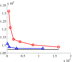
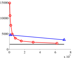
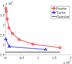
Testing classification error
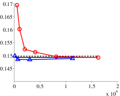
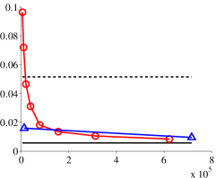
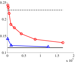
	Computational cost	Computational cost	Computational cost

Figure 1: Primal objectives and testing classification errors for various numbers of Fourier and Taylor features. For the Fourier features, the markers correspond to numbers of features which are powers of two, starting at $32$. For Taylor, each marker corresponds to a degree, starting at $2$. The cost of calculating $\tilde{\phi}$, in units of floating point operations, is displayed on the horizontal axis. The solid black lines are the primal objective function value and testing classification error achieved by the optimal solution to the Gaussian kernel SVM problem, while the dashed lines in the bottom plots are the testing classification error achieved by a linear SVM.

Cov1
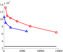
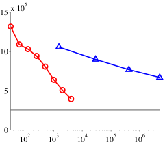
Primal objective		Primal objective		Average $\left|K-\tilde{K}\right|$
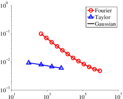
	Computational cost		# features		Computational cost
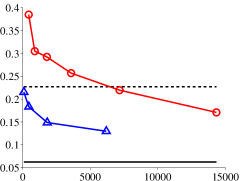
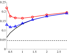
Testing classification error		Testing classification error		Average $\left|K-\tilde{K}\right|$
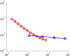
	Computational cost		$\sigma$		# features

Figure 2: Left column: same as Figure 1. Top middle: primal objective as a function of the total number of features (in log scale). Bottom middle: test error as a function of the Gaussian kernel parameter $\sigma$, for Taylor and random Fourier expansions of the same computational cost, compared with the true Gaussian kernel. The dot-dashed line indicates the performance of a 1-NN classifier, trained using the ANN library (Arya and Mount, 1993; Mount and Arya, 2006; Bagon, 2009). Right column: average value of the approximation error $|K\left(x,x^{\prime}\right)-\tilde{K}\left(x,x^{\prime}\right)|$ over 100000 randomly chosen pairs of training vectors, in terms of both computational cost and total number of features.

For each of the data sets, we compared the value of the (primal) SVM objective and the classification performance (on the test set) achieved using varying numbers of Taylor and Fourier features. Results are reported in Figure 1 and in the left column of Figure 2. We report results in units of the number of floating-point operations required to calculate each feature vector, taking into account sparsity, as discussed in Section 4. As was discussed earlier, this is the dominant cost in stochastic optimization methods such as Pegasos (Shalev-Shwartz et al., 2007) and stochastic dual coordinate ascent (Hsieh et al., 2008), which are the fastest methods of training large-scale liner SVMs. We used a fairly optimized SGD implementation into which the explicit feature vector calculations were integrated. Our actual runtimes are indeed in line with the calculated computational costs (we prefer reporting the theoretical cost as it is not implementation or architecture dependent).

As can be seen from Figures 1 and 2, the computational cost required to obtain the same SVM performance is typically lower when using the Taylor features than the Fourier features, despite the exponential growth of the number of features as a function of the degree. The exception is the MNIST dataset, which has a fairly high number (over 150) of non-zero dimensions per data point, yielding an extremely sharp increase in the computational costs of higher-degree Taylor feature expansions.

To better appreciate the difference between the dependence on the number of features and that on the computational cost we include more detailed results for the Cov1 dataset, in Figure 2. Here we again plot the value of the SVM objective, this time both as function of the number of features and as a function of the computational cost. As expected, the Fourier features perform much better as a function of the number of features, but, as argued earlier, we should be more concerned with the cost of calculating them. In order to directly measure how well each feature representation approximates the Gaussian kernel, we also include in Figure 2 a comparison of the average approximation error.

Next, we consider the effect of the bandwidth parameter $\sigma$ on the Taylor and Fourier approximations—note that the theoretical analysis for both methods deteriorates significantly when the bandwidth decreases. This is verified in the bottom-middle plot of Figure 2, which shows that the (test) classification error of the two approximations (with the same fixed computational budget) deteriorates, relative to that of the true Gaussian SVM, as the bandwidth decreases. This deterioration can be observed on other data sets as well. On Cov1, the deterioration is so strong that even though the generalization performance of the true Gaussian Kernel SVM keeps improving as the bandwidth decreases, the test errors for both approximations actually start increasing fairly quickly. It should be noted that Cov1 is atypical in this regard: nearest-neighbor classification achieves almost optimal results on this dataset (the dot-dashed line in the bottom-middle plot of Figure 2), and so decreasing the bandwidth, which approximates the nearest-neighbor classifier, is beneficial. In contrast, on the data sets in Figure 1, the optimal bandwidth for the Gaussian kernel is large enough to allow good approximation by the Fourier and Taylor approximations.

Finally, in order to get some perspective on the real-world benefit of the Taylor features, we also report actual runtimes for a large scale realistic example. We compared training times for the Gaussian kernel and the Taylor features, on the full TIMIT dataset, where the goal was framewise phoneme classification, i.e., given a 10 ms frame of speech the goal is to predict the uttered phoneme from a set of 39 phoneme symbols. We used the standard split of the dataset to training, validation test sets, and extracted MFCC features. With this set of acoustic features the common practice in to use the Gaussian kernel. Its bandwidth was selected on the validation set to be $\sigma^{2}=19$. The training set includes 1.1 million examples, and existing SVM libraries such as SVMLIB or SVMLight failed to converge in a reasonable amount of time (see the training time in Salomon et al. (2002)). Using our own implementation with the exact Gaussian kernel and stochastic dual coordinate ascent, the training took 313 hours (almost two weeks) on 2GHz Intel Core 2 (using one core). Using the same implementation with the kernel function replaced by its degree-$3$ Taylor approximation, the training took only 53 hours. The results were almost the same: multiclass accuracy of $69.6\%$ for the approximated kernel and $69.8\%$ for the Gaussian kernel. These are state-of-the-art results for this dataset (Salomon et al., 2002; Graves and Schmidhuber, 2005).

6 Relationship to the Polynomial Kernel

Like the Taylor feature representation of the Gaussian kernel, the standard polynomial kernel of degree $r$:

$$K\left(x,x^{\prime}\right)=\left(\left\langle x,x^{\prime}\right\rangle+c\right)^{r}$$ (14)

corresponds to a feature space containing all monomials of degree at most $r$. More specifically, the features corresponding to the kernel (14) can be written as:

$$\phi_{k,j}\left(x\right)=\sqrt{{r\choose k}c^{r-k}}\prod_{i=1}^{k}x_{j_{i}}$$ (15)

where, as in (9), $k=0,\ldots,r$ and $j\in\left[d\right]^{k}$ enumerates over all selections of $k$ coordinates in $\mathbf{x}$. The difference, relative to the Taylor approximation to the Gaussian, is only in a per-example overall scaling factor based on $\|\mathbf{x}\|$, and in a different per-degree factor (which depends only on the degree $k$). This weighting by a degree-dependent factor should not be taken lightly, as it affects regularization, which is key to SVM training–features scaled by a larger factor are “cheaper” to use, compared to those scaled by a very small factor. Comparing the degree-dependent scaling in the two feature representations ((9) and (15)), we observe that the higher degrees are scaled by a much smaller factor in the Taylor features, owing to the rapidly decreasing dependence on $1/\sqrt{k!}$. This means that higher degree monomials are comparatively much more expensive for use in the Taylor features, and that the learned predictor likely relies more on lower degree monomials.

Table 2: Comparison of the Gaussian kernel and its Taylor approximation to the polynomial kernel $K\left(x,y\right)=\left(\left\langle x,y\right\rangle+1\right)^{d}$, after scaling the data to have unit average squared norm. Here, $d$ is the degree of the polynomial. The reported test errors are the minima over parameter choices taken from a coarse power-of-two based grid, within which the reported parameters are well inside the interior. Gaussian kernel SVMs were optimized using our GPU optimizer, while the others were optimized by running Pegasos for $100$ epochs.

	Gaussian			Taylor				Polynomial
Dataset	$C$	$\sigma^{2}$	Test error	degree	$C$	$\sigma^{2}$	Test error	degree	$C$	Test error
Adult	4	100	14.9%	4	8	200	14.7%	4	4	14.8%
MNIST	8	100	0.42%	2	2048	200	0.54%	2	256	0.58%
TIMIT	2	40	10.8%	3	8	200	11.4%	3	64	11.6%
Cov1	16	0.03125	3.3%	4	128	0.5	12.3%	4	512	13.6%

Nevertheless, the space of allowed predictors is nearly the same with both types of features, raising the question of how strong the actual effect of the different per-degree weighting is. The fact that all of the features in the Taylor representation are scaled by a factor depending on $\|x\|$ should make little difference on many datasets, as it affects all of the features of a given example equally. Likewise, if most of the used features are of the same degree, then we could perhaps correct for the degree-based scaling by changing the regularization parameter. The problem, of course, is searching for and selecting this parameter.

We checked if we could find a substantial difference in performance between the Taylor and standard polynomial features. Because the dependence on the regularization parameter necessitated a search over the parameter space, we conducted a rough experiment in which we tried different parameters, and compared the best error achieved on the test set using the true Gaussian kernel, a Taylor approximation, and a standard polynomial kernel of the same degree. The results are summarized in Table 2. These experiments indicate that the standard polynomial features might be sufficient for approximating the Gaussian. Still, the Taylor features are just as easy to compute and use, and have the advantage that they use the same parameters as the Gaussian kernel. Hence, if we already have a sense of good bandwidth and $C$ parameters for the Gaussian kernel, we can use the same values for the Taylor approximation.

7 Summary

The use of explicit monomial features of the form of (15) has been discussed recently as a way of speeding up training with the polynomial kernel (Sonnenburg and Franc, 2010; Chang et al., 2010). Our analysis and experiments indicate that a similar monomial representation is also suitable for approximating the Gaussian kernel. We argue that such features might often be preferable to the random Fourier features recently suggested by Rahimi and Recht (2007). This is especially true on sparse datasets with a moderate number (up to several dozen) of non-zero dimensions per data point.

Although we have only focused on binary classification, it is important to note that the this explicit feature representation can be used anywhere else $\ell_{2}$ regularization is used. This includes multiclass, structured and latent SVMs. The use of such feature expansions might be particularly beneficial to structured SVMs, since these problems are hard to solve with only a kernel representation.

References

- Arya and Mount [1993] S. Arya and D. M. Mount. Approximate nearest neighbor queries in fixed dimensions. In Proc. SODA 1993, pages 271–280, 1993.
- Bagon [2009] S. Bagon. Matlab class for ANN, February 2009. URL http://www.wisdom.weizmann.ac.il/~bagon/matlab.html.
- Balcan et al. [2006] M.-F. Balcan, A. Blum, and S. Vempala. Kernels as features: On kernels, margins, and low-dimensional mappings. In Machine Learning, volume 65 (1), pages 79–94. Springer Netherlands, October 2006.
- Bordes et al. [2005] A. Bordes, S. Ertekin, J. Weston, and L. Bottou. Fast kernel classifiers with online and active learning. JMLR, 6:1579–1619, September 2005.
- Chang et al. [2010] Y.-W. Chang, C.-J. Hsieh, K.-W. Chang, M. Ringgaard, and C.-J. Lin. Training and testing low-degree polynomial data mappings via linear SVM. JMLR, 99:1471–1490, August 2010.
- Fine and Scheinberg [2002] S. Fine and K. Scheinberg. Efficient SVM training using low-rank kernel representations. JMLR, 2:243 – 264, March 2002.
- Graves and Schmidhuber [2005] A. Graves and J. Schmidhuber. Framewise phoneme classification with bidirectional LSTM and other neural network architectures. Neural Networks, 18:602–610, 2005.
- Hsieh et al. [2008] C.-J. Hsieh, K.-W. Chang, C.-J. Lin, S. S. Keerthi, and S. Sundararajan. A dual coordinate descent method for large-scale linear SVM. In Proc. ICML 2008, pages 408–415, 2008.
- Mount and Arya [2006] D. M. Mount and S. Arya. ANN: A library for approximate nearest neighbor searching, August 2006. URL http://www.cs.umd.edu/~mount/ANN.
- Platt [1998] J. C. Platt. Fast training of support vector machines using Sequential Minimal Optimization. In B. Schölkopf, C. Burges, and A. Smola, editors, Advances in Kernel Methods - Support Vector Learning. MIT Press, 1998.
- Rahimi and Recht [2007] A. Rahimi and B. Recht. Random features for large-scale kernel machines. In Proc. NIPS 2007, 2007.
- Rahimi and Recht [2008] A. Rahimi and B. Recht. Uniform approximation of functions with random bases. In Proceedings of the 46th Annual Allerton Conference, 2008.
- Salomon et al. [2002] J. Salomon, S. King, and M. Osborne. Framewise phone classification using support vector machines. In Proceedings of the Seventh International Conference on Spoken Language Processing, pages 2645–2648, 2002.
- Shalev-Shwartz et al. [2007] S. Shalev-Shwartz, Y. Singer, and N. Srebro. Pegasos: Primal Estimated sub-GrAdient SOlver for SVM. In Proc. ICML 2007, pages 807–814, 2007.
- Shalev-Shwartz et al. [2010] S. Shalev-Shwartz, Y. Singer, N. Srebro, and A. Cotter. Pegasos: Primal Estimated sub-GrAdient SOlver for SVM. In Mathematical Programming, pages 1–34. Springer, October 2010.
- Sonnenburg and Franc [2010] S. Sonnenburg and V. Franc. COFFIN: a computational framework for linear SVMs. In Proc. ICML 2010, 2010.
- Xu et al. [2004] J.-W. Xu, P. P. Pokharel, K.-H. Jeong, and J. C. Principe. An explicit construction of a reproducing Gaussian kernel Hilbert space. In Proc. NIPS 2004, 2004.
- Yang et al. [2006] C. Yang, R. Durasiwami, and L. Davis. Efficient kernel machine using the improved fast Gaussian transform. In Proc. IEEE International Conference on Acoustic, Speech and Signal Processing, 2006.