The Photometric Classification Server for Pan-STARRS1

Abstract

The Pan-STARRS1 survey is obtaining multi-epoch imaging in 5 bands ($g_{\rm P1}$$r_{\rm P1}$$i_{\rm P1}$$z_{\rm P1}$$y_{\rm P1}$) over the entire sky North of declination $-30\deg$. We describe here the implementation of the Photometric Classification Server (PCS) for Pan-STARRS1. PCS will allow the automatic classification of objects into star/galaxy/quasar classes based on colors, the measurement of photometric redshifts for extragalactic objects, and constrain stellar parameters for stellar objects, working at the catalog level. We present tests of the system based on high signal-to-noise photometry derived from the Medium Deep Fields of Pan-STARRS1, using available spectroscopic surveys as training and/or verification sets. We show that the Pan-STARRS1 photometry delivers classifications and photometric redshifts as good as the Sloan Digital Sky Survey (SDSS) photometry to the same magnitude limits. In particular, our preliminary results, based on this relatively limited dataset down to the SDSS spectroscopic limits and therefore potentially improvable, show that stars are correctly classified as such in 85% of cases, galaxies in 97% and QSOs in 84%. False positives are less than 1% for galaxies, $\approx 19$% for stars and $\approx 28$% for QSOs. Moreover, photometric redshifts for 1000 luminous red galaxies up to redshift 0.5 are determined to 2.4% precision (defined as $1.48\times Median|z_{phot}-z_{spec}|/(1+z)$) with just 0.4% catastrophic outliers and small (-0.5%) residual bias. For bluer galaxies up to the same redshift the residual bias (on average -0.5%) trend, percentage of catastrophic failures (1.2%) and precision (4.2%) are higher, but still interestingly small for many science applications. Good photometric redshifts (to 5%) can be obtained for at most 60% of the QSOs of the sample. PCS will create a value added catalog with classifications and photometric redshifts for eventually many millions sources.

1 INTRODUCTION

Pan-STARRS1, the prototype of the Panoramic Survey Telescope and Rapid Response System, started scientific survey operations in May 2010 and is producing a 5 band ($g_{\rm P1}$$r_{\rm P1}$$i_{\rm P1}$$z_{\rm P1}$$y_{\rm P1}$) imaging for 3/4 of the sky that will be $\approx 1$ mag deeper than the Sloan Digital Sky Survey (SDSS, York et al., 2000; Abazajian et al., 2009) at the end of the foreseen 3 years of operations. Approximately two hundred million galaxies, a similar number of stars, about a million quasars and $\approx 7000$ Type Ia Supernovae will be detected. In addition to the search for so-called “killer asteroids”, the science cases driving Pan-STARRS1 are both galactic and extragalactic. Extragalactic goals range from Baryonic Acoustic Oscillations and growth of structure, to weak shear, galaxy-galaxy lensing and lensing tomography. All rely on the determination of accurate photometric redshifts for extremely large numbers of galaxies. The galactic science cases focus on the search for very cool stars and the structure of the Milky Way, requiring good star/galaxy (photometric) classification and constraints on stellar parameters. Further science goals, such as the detection of high redshift quasars and galaxies, quasar/quasar and quasar/galaxy clustering, or the study of how galaxies evolve with cosmic time profit from the availability of good photometric redshifts and star/galaxy photometric classification. Therefore in the last years we have designed (Saglia, 2008; Snigula et al., 2009) and implemented the Photometric Classification Server (PCS) for Pan-STARRS1 to derive and administrate photometric redshift estimates and probability distributions; star/galaxy classification and stellar parameters for extremely large datasets. The present paper describes the system and its performances in various tests.

The structure of the paper is as follows. The Pan-STARRS1 system is sketched out in Section 2, the observations we used are described in Section 3 and data processing is outlined in Section 4. Section 5 presents the PCS system, its algorithms and components, and the implementation. Section 6 discusses the tests of the system, which is followed by our conclusions in Section 7.

2 The Pan-STARRS1 Telescope, Camera, and Image Processing

The Pan-STARRS1 system is a high-etendue wide-field imaging system, designed for dedicated survey operations. The system is installed on the peak of Haleakala on the island of Maui in the Hawaiian island chain. Routine observations are conducted remotely, from the Advanced Technology research Center in Pukalani. We provide below a terse summary of the Pan-STARRS1 survey instrumentation. A more complete description of the Pan-STARRS1 system, both hardware and software, is provided by Kaiser et al. (2010). The survey philosophy and execution strategy are described by Chambers et al. (in prep).

The Pan-STARRS1 optical design (Hodapp et al., 2004) uses a 1.8 meter diameter primary mirror, and a 0.9 m secondary. The resulting converging beam then passes through two refractive correctors, a $48$ cm $\times~{}48$ cm interference filter, and a final refractive corrector that is the dewar window. The entire optical system delivers an $f$/4.4 beam and an image with a diameter of 3.3 degrees, with low distortion. The Pan-STARRS1 imager (Tonry & Onaka, 2009) comprises a total of 60 detectors, with $4800\times 4800$ 10 $\mu$m pixels that each subtend 0.258 arcsec. The detectors are back-illuminated CCDs, manufactured by Lincoln Laboratory, and read out using a StarGrasp CCD controller, with a readout time of 7 seconds for a full unbinned image. Initial performance assessments are presented by Onaka et al. (2008).

The Pan-STARRS1 observations are obtained through a set of five broadband filters, which we have designated as $g_{\rm P1}$, $r_{\rm P1}$, $i_{\rm P1}$, $z_{\rm P1}$, and $y_{\rm P1}$. Under certain circumstances Pan-STARRS1 observations are obtained with a sixth, “wide” filter designated as $w_{\rm P1}$ that essentially spans $g_{\rm P1}$, $r_{\rm P1}$, and $i_{\rm P1}$. Although the filter system for Pan-STARRS1 has much in common with that used in previous surveys, such as the SDSS, there are important differences. The $g_{\rm P1}$ filter extends 20 nm redward of $g_{SDSS}$, paying the price of 5577Å sky emission for greater sensitivity and lower systematics for photometric redshifts, and the $z_{\rm P1}$ filter is cut off at 930 nm, giving it a different response from $z_{SDSS}$. SDSS has no corresponding $y_{\rm P1}$ filter, while Pan-STARRS1 is lacking u-band photometry that SDSS provides. Further information on the passband shapes is described in Stubbs et al. (2010). Provisional response functions (including 1.3 airmasses of atmosphere) are available at the project’s web site . Photometry is in the “natural” Pan-STARRS1 system, $m=-2.5log(flux)+m^{\prime}$, with a single zeropoint adjustment $m^{\prime}$ made in each band to conform to the AB magnitude scale (Tonry et al., in prep). Pan-STARRS1 magnitudes are interpreted as being at the top of the atmosphere, with 1.3 airmasses of atmospheric attenuation being included in the system response function. No correction for Galactic extinction is applied to the Pan-STARRS1 magnitudes. We stress that, like SDSS, Pan-STARRS1 uses the AB photometric system and there is no arbitrariness in the definition. Flux representations are limited only by how accurately we know the system response function vs. wavelength.

Images obtained by the Pan-STARRS1 system are processed through the Image Processing Pipeline (IPP) (Magnier, 2006), on a computer cluster at the Maui High Performance Computer Center. The pipeline runs the images through a succession of stages, including flat-fielding (“de-trending”), a flux-conserving warping to a sky-based image plane, masking and artifact removal, and object detection and photometry. The IPP also performs image subtraction to allow for the prompt detection of variables and transient phenomena. Mask and variance arrays are carried forward at each stage of the IPP processing. Photometric and astrometric measurements performed by the IPP system are described in Magnier (2007) and Magnier et al. (2008) respectively.

The details of the photometric calibration and the Pan-STARRS1 zeropoint scale will be presented in a subsequent publication (Tonry et al., in prep), and Magnier et al. (in prep) will provide the application to a consistent photometric catalog over the 3/4 sky observed by Pan-STARRS1.

3 Observations

This paper uses images and photometry from the Pan-STARRS1 Medium-Deep Field survey. In addition to covering the sky at $\delta>-30\deg$ in 5 bands, the Pan-STARRS1 survey has obtained deeper multi-epoch images in the Pan-STARRS1 $g_{\rm P1}$, $r_{\rm P1}$, $i_{\rm P1}$, $z_{\rm P1}$ and $y_{\rm P1}$ bands of the fields listed in Table 1. The typical Medium-deep cadence of observations is $8\times 113$ s in the $g_{\rm P1}$ and $r_{\rm P1}$ bands the first night, $8\times 240$ s in the $i_{\rm P1}$ band the second night, $8\times 240$ s in the $z_{\rm P1}$ band the third night, $8\times 113$ s in the $g_{\rm P1}$ and $r_{\rm P1}$ bands in the forth night, and on each of the 3 nights on either side of Full Moon $8\times 240$ s in the $y_{\rm P1}$ band. The 5 $\sigma$ point source detection limits achieved in the various $g_{\rm P1}$$r_{\rm P1}$$i_{\rm P1}$$z_{\rm P1}$$y_{\rm P1}$ bands, as well as other statistics of potential interest, are presented in Table 2 for the co-added stacks. They represent the depth of stacks at the time of writing, as observations are still on-going. In the following we will only consider the fields MDF03 to 10, that overlap with SDSS.

Table 1: Pan-STARRS1 Medium-Deep Field Centers.

Field	Alternative names	RA (degrees, J2000)	Dec (degrees, J2000)
MDF01	MD01, PS1-MD01	35.875	$4.250$
MDF02	MD02, PS1-MD02	53.100	$-27.800$
MDF03	MD03, PS1-MD03	130.592	$44.317$
MDF04	MD04, PS1-MD04	150.000	$2.200$
MDF05	MD05, PS1-MD05	161.917	$58.083$
MDF06	MD06, PS1-MD06	185.000	$47.117$
MDF07	MD07, PS1-MD07	213.704	$53.083$
MDF08	MD08, PS1-MD08	242.787	$54.950$
MDF09	MD09, PS1-MD09	334.188	$0.283$
MDF10	MD10, PS1-MD10	352.312	$-0.433$

Table 2: Pan-STARRS1 MDF Statistics, Apr 2009–Apr 2011.

Field	Filter	$N$	$\log t$	$PSF$	$\langle w\rangle$	$m_{lim}$	Field	Filter	$N$	$\log t$	$PSF$	$\langle w\rangle$	$m_{lim}$
MDF01	$g_{\rm P1}$	42	4.7	1.25	1.55	24.5	MDF06	$g_{\rm P1}$	38	4.6	1.25	1.56	24.4
MDF01	$r_{\rm P1}$	42	4.7	1.15	1.35	24.4	MDF06	$r_{\rm P1}$	39	4.6	1.18	1.45	24.2
MDF01	$i_{\rm P1}$	41	4.9	1.05	1.27	24.4	MDF06	$i_{\rm P1}$	41	4.9	1.14	1.39	24.3
MDF01	$z_{\rm P1}$	41	4.9	1.03	1.24	23.9	MDF06	$z_{\rm P1}$	38	4.9	1.05	1.30	23.7
MDF01	$y_{\rm P1}$	21	4.6	0.95	1.17	22.4	MDF06	$y_{\rm P1}$	24	4.7	1.00	1.25	22.4
MDF02	$g_{\rm P1}$	30	4.5	1.31	1.79	24.2	MDF07	$g_{\rm P1}$	36	4.5	1.23	1.68	24.3
MDF02	$r_{\rm P1}$	29	4.5	1.20	1.74	24.1	MDF07	$r_{\rm P1}$	39	4.5	1.13	1.46	24.2
MDF02	$i_{\rm P1}$	30	4.8	1.11	1.50	24.2	MDF07	$i_{\rm P1}$	39	4.9	1.14	1.44	24.2
MDF02	$z_{\rm P1}$	33	4.8	1.06	1.30	23.6	MDF07	$z_{\rm P1}$	43	4.9	1.08	1.37	23.7
MDF02	$y_{\rm P1}$	16	4.5	1.14	1.42	22.1	MDF07	$y_{\rm P1}$	30	4.8	1.01	1.28	22.5
MDF03	$g_{\rm P1}$	38	4.6	1.18	1.44	24.5	MDF08	$g_{\rm P1}$	38	4.5	1.27	1.68	24.3
MDF03	$r_{\rm P1}$	37	4.6	1.09	1.28	24.4	MDF08	$r_{\rm P1}$	38	4.5	1.14	1.47	24.2
MDF03	$i_{\rm P1}$	41	4.9	1.06	1.31	24.4	MDF08	$i_{\rm P1}$	33	4.8	1.07	1.34	24.2
MDF03	$z_{\rm P1}$	42	5.0	1.03	1.27	23.9	MDF08	$z_{\rm P1}$	40	4.9	1.09	1.39	23.7
MDF03	$y_{\rm P1}$	20	4.6	1.00	1.36	22.4	MDF08	$y_{\rm P1}$	32	4.9	0.98	1.27	22.7
MDF04	$g_{\rm P1}$	35	4.6	1.17	1.52	24.5	MDF09	$g_{\rm P1}$	34	4.5	1.26	1.55	24.3
MDF04	$r_{\rm P1}$	37	4.6	1.09	1.46	24.3	MDF09	$r_{\rm P1}$	33	4.5	1.15	1.42	24.1
MDF04	$i_{\rm P1}$	35	4.9	1.07	1.35	24.3	MDF09	$i_{\rm P1}$	34	4.8	1.02	1.36	24.3
MDF04	$z_{\rm P1}$	28	4.8	1.03	1.32	23.6	MDF09	$z_{\rm P1}$	34	4.8	1.02	1.26	23.7
MDF04	$y_{\rm P1}$	8	4.3	1.03	1.21	22.0	MDF09	$y_{\rm P1}$	12	4.3	0.94	1.12	22.0
MDF05	$g_{\rm P1}$	42	4.6	1.24	1.58	24.4	MDF10	$g_{\rm P1}$	30	4.5	1.26	1.60	24.2
MDF05	$r_{\rm P1}$	40	4.6	1.17	1.46	24.3	MDF10	$r_{\rm P1}$	33	4.5	1.18	1.53	24.2
MDF05	$i_{\rm P1}$	34	4.8	1.06	1.44	24.3	MDF10	$i_{\rm P1}$	30	4.8	1.01	1.31	24.2
MDF05	$z_{\rm P1}$	27	4.8	0.99	1.27	23.6	MDF10	$z_{\rm P1}$	28	4.8	1.03	1.24	23.6
MDF05	$y_{\rm P1}$	17	4.6	1.02	1.33	22.3	MDF10	$y_{\rm P1}$	11	4.4	0.96	1.22	22.2

4 Data processing

The Pan-STARRS1 IPP system performed flatfielding on each of the individual images, using white light flatfield images from a dome screen, in combination with an illumination correction obtained by rastering sources across the field of view. Bad pixel masks were applied, and carried forward for use at the stacking stage. After determining an initial astrometric solution, the flat-fielded images were then warped onto the tangent plane of the sky, using a flux conserving algorithm. The plate scale for the warped images is 0.200 arcsec/pixel. The IPP software for stacking and photometry is still being optimized. Therefore, for this paper we generate stacks using customized software from one of us (JT) and produce aperture photometry catalogs running Sextractor (Bertin & Arnoux, 1996) on each stacked image independently. At a second stage we match the catalogs requiring a detection in each band within a one arcsec radius. For simplicity we use a rather large aperture radius (7.4 arcsec) for our photometry and we do not apply any seeing correction, even if for some of the Medium-Deep fields slight variations in the FWHM between the filters are observed (see Table 2). In the production mode of operations IPP will provide stacks with homogenized PSF, where forced photometry will be performed at each point where a detection in one of the unconvolved stacks is reported. The catalogs will be ingested in the Published Science Products Subsystem (PSPS, Heasley, 2008), the database that will serve the scientific community with the final Pan-STARRS1 products. Note that at present PCS uses fluxes and flux ratios, but no morphological information, such as spatial extent or shape.

5 The PCS system

The science projects described in the Introduction define broadly the requirements for the PCS. It should provide software tools to compute: (a) photometric, color-based star/QSO/galaxy classification (i.e., morphological classifiers based on sizes and shapes are not part of PCS, even if this additional information could and probably will be added in the future), (b) best fitting spectral energy distribution and photometric redshifts (photo-z) with errors for (reddish) galaxies. Furthermore (c), (a subset of the stellar parameters) best-fitting temperature, metallicity, gravity and interstellar extinction with errors for (hot and cool) stars should be provided. The codes should be interfaced to the PSPS database and to the dataserver of IPP and results written directly into PSPS (i.e. photo-z with errors) and into additional databases linked to the PSPS, dubbed MYDB.

In the following, we first describe the algorithms that implement (a) and (b) (Section 5.1), then the system components (i.e. the different independent pieces of code that make PCS, Section 5.2), and finally its implementation (Section 5.3). Point (c) is still under development and will be described in a future paper. Presently, (a) and (b) do not communicate with each other and work independently. We plan to upgrade the package in the future, merging in an optimal way the classification information coming from both approaches, and using it to improve the determination of photometric redshifts.

PCS is designed to work with catalogs providing fluxes in the $g_{\rm P1}$, $r_{\rm P1}$, $i_{\rm P1}$, $z_{\rm P1}$, $y_{\rm P1}$ bands and their errors (further bands can be added if available through external datasets). Optimal performances are expected for objects with good photometry in all Pan-STARRS1 bands, but (somewhat deteriorated) output can be obtained even in the absence of some bands or low signal-to-noise data.

5.1 The algorithms

5.1.1 SVM for PanDiSC

There is an ongoing trend in astronomy towards larger and deeper surveys. The natural consequence of this is the advent of very large datasets. There is therefore a need for automated data handling, or data mining, techniques to handle this data volume. Automated source classifiers based on photometric observations can provide class labels for catalogues, or be used to recover objects for further study according to various criteria.

The SDSS used a selection of algorithms to classify catalogue objects and select followup targets (Adelman-McCarthy et al., 2006). Methods based on colour selection were particularly employed for finding probable quasars (Richards et al., 2002). More recently, Gao, Zhang & Zhao (2008), Richards et al. (2009a) and Richards et al. (2009b) have used Kernel density estimators for quasar selection in SDSS data. Galaxy classification is usually primarily based on detecting source extension by comparing PSF magnitudes with magnitudes based on various profile models. For examples of Galaxy classification see Vasconcellos et al. (2011) who used decision trees for star-galaxy separation in SDSS, or Henrion et al. (2011), who used a Bayesian method for star-galaxy separation in SDSS and UKIDSS. Tzalmantza et al. (2007) and Tzalmantza et al. (2009) have developed a test library and selection methods for identifying galaxies in the forthcoming Gaia mission.

Lee et al. (2008) identified various stellar populations for followup in the SEGUE survey from SDSS photometry. Other attempts to identify stellar populations from photometric data include Smith et al. (2010), who investigated the use of several automated classifiers on SDSS data to identify BHB stars, and Klement et al. (2011) who used a support vector machine to separate field giants from dwarfs using photometric data from a range of surveys. Marengo and Sanchez (2009) used a kNN technique to search for brown dwarfs in Spitzer data.

Finally, it should be mentioned that there is a whole industry of finding ways to classify various types of variable objects based on their photometric light curves. See for example Dubath et al. (2011) for classification of various stellar types with a Random forest method, or Schmidt et al. (2010) who developed a method for separating quasars from variable stars based on a structure function fit.

The Pan-STARRS1 Discrete Source Classifier (PanDiSC) used here is based on a support vector machine (SVM), a statistical learning algorithm. SVM works by learning a nonlinear boundary to optimally separate two or more classes of objects. Here it takes as input the 4 Pan-STARRS1 $g_{\rm P1}$-$r_{\rm P1}$, $r_{\rm P1}$-$i_{\rm P1}$, $i_{\rm P1}$-$z_{\rm P1}$, $z_{\rm P1}$-$y_{\rm P1}$ colors. PanDiSC is based on the Discrete Source Classifier under development for the purpose of classifying low resolution spectroscopy from Gaia (Bailer-Jones et al., 2008). The SVM runs in the PanDiSC component of PCS (see Section 5.2). The SVM implementation used is libSvm (Chang & Lin, 2011), available at http://www.csie.ntu.edu.tw/$\tilde{~{}}$cjlin/libsvm. Probabilities are calculated by modeling the density of data points on either side of the decision boundary, according to the method of Platt (1999), and the multiclass probabilities are obtained by pairwise coupling, as described by Wu, Lin & Weng (2004). PanDiSC chooses the highest membership probability from the eventual output for each source and assigns the membership to the star/QSO/galaxy class accordingly.

The SVM is trained on a sample of objects with Pan-STARRS1 photometry and spectroscopic classification, to which the parameters $\gamma$ (the scaling factor) and $C$ (the regularisation cost) of the radial basis functions (RBF) kernel are tuned using a downhill simplex algorithm (Smith, 2009). The system has been applied to the SDSS DR6 dataset (Elting et al., 2008) producing an excellent confusion matrix (i.e. high accuracy of classification, $\geq 96$%, and low percentage of false positives, $\approx 29$% for the stellar catalog, 0.5% for the galaxy catalog, 10% for the QSO catalog). The code is a compiled Java program.

5.1.2 PhotoZ for PanZ

In the last decade several efficient codes for the determination of photometric redshifts have been developed, based either on empirical methods, or template fitting. In the first case one tries to parametrize the low-dimensional surface in color-redshift space that galaxies occupy using low-order polynomials, nearest-neighbor searches or neural networks (Csabai et al., 2003; Collister & Lahav, 2004). These codes extract the information directly from the data, given an appropriate training set with spectroscopic information. Template fitting methods work instead with a set of model spectra from observed galaxies and stellar population models (Padmanabhan et al., 2005; Ilbert et al., 2006; Mobasher et al., 2007; Ilbert et al., 2009; Pello et al., 2009).

The PhotoZ code used in the PanZ component of the PCS system (see Section 5.2) belongs to this last category and is described in Bender et al. (2001). The code estimates redshifts $z$ by comparing T, a set of discrete template SEDs, to the broadband photometry of the (redshifted) galaxies. For each SED the full redshift posterior probability function including priors for redshift, absolute luminosity, and SED probability is computed using Bayes’ theorem:

$$P(z,T|F,M,...)\propto p(F|z,T)p(z,T|M),$$ (1)

where $F$ is the vector of measured fluxes in different bands, $M$ the galaxy absolute magnitude in the B band (see below), $p(z,T|M)$ the prior distribution and $p(F|z,T)\propto exp(-\chi^{2}/2)$ is the probability of obtaining a normalized $\chi^{2}$ for the given dataset, redshift and template $T$. In detail, we compute $\chi^{2}$ as:

$$\chi^{2}=\sum_{i}\frac{(\alpha f_{i,mod}(z)-f_{i,dat})^{2}}{(w_{i}\alpha f_{i,mod})^{2}+\Delta f_{i,dat}^{2}},$$ (2)

where $f_{i,mod}(z)$ and $f_{i,dat}$ are the fluxes of the templates (at the redshift $z$) and of the data in a filter band $i$, and $\Delta f_{i,dat}$ are the errors on the data. The model weights $w_{i}$ quantify the intrinsic uncertainties of the SEDs for the specific filter $i$, presently they are all set to $w_{i}=0.1$. The normalization parameter $\alpha$ is computed by minimizing $\chi^{2}$ at each choice of parameters.

The priors are (products of) parameterized functions of the type:

$$p(y)\propto y^{n}exp\left[-ln(2)\left(\frac{y-\hat{y}}{\sigma_{y}}\right)^{p}\right],$$ (3)

where the variable $y$ stands for redshift or absolute magnitudes. Typically we use $n=0$, $p=6$ or $8$, and $\hat{y}$ and $\sigma_{y}$ with appropriate values for mean redshifts and ranges, or mean absolute B magnitudes and ranges, which depend on the SED type. The absolute magnitudes of the objects are computed on the fly for the considered rest-frame SED, normalization $\alpha$ and redshift, using the standard cosmological parameters ($\Omega_{m}=0.3$, $\Lambda=0.7$, $H_{0}=70$ Mpc/(km/s)). The use of fluxes $f_{i,dat}$ instead of the magnitudes allows us to take into account negative datapoints and upper limits.

The set of galaxy templates is semi-empirical and can be optimized through an interactive comparison with a spectroscopic dataset. The original set (Bender et al., 2001; Gabasch et al., 2004) includes 31 SEDs describing a broad range of galaxy spectral types, from early to late to star-bursting objects. Recently, we added a set of SEDs tailored to fit Luminous Red Galaxies (LRGs, Eisenstein et al., 2001), see Greisel et al. (in prep), and one SED to represent an average QSO spectrum. This was obtained by averaging the low redshift HST composite of Telfer et al. (2002) and the SDSS median quasar composite of Vander Berk et al. (2001). Furthermore, the method also fits a set of stellar templates, allowing a star/galaxy classification and an estimate of the line-of-sight extinction for stellar objects. The templates cover typically the wavelength range $\lambda=900$ Å up to 25000 Å (with the QSO template covering instead 300-8000 Å) and are sampled with a step typically 10 Å wide (varying from 5 to 20 Å; the QSO SED has $\Delta\lambda=1$ Å).

The method has been extensively tested and applied to several photometric catalogs with spectroscopic follow-up (Gabasch et al., 2004; Feulner et al., 2005; Gabasch et al., 2008; Brimioulle et al., in prep). Given a (deep) photometric dataset covering the wavelength range from the U to the K band, excellent photometric redshifts with $(z_{phot}-z_{spec})/(1+z)\sim 0.03$ up to $z\approx 5$ with at most a few percent catastrophic failures can be derived for every SED type. With the help of appropriate priors, photometric redshifts accurate to 2% (in $(z_{phot}-z_{spec})/(1+z_{spec})$) with just 1% outliers (see Sect. 6 for definitions) are obtained for LRGs using the ugriz SDSS photometric dataset (Greisel et al., in prep). This is the first time we attempt to determine the photometric redshifts of QSOs. We couple the available SED to a strong prior in luminosity that dampens its probability as soon as the predicted B band absolute magnitude is fainter than -24.

The code is in C++. A Fortran version is available as implemented under Astro-WISE (Valentijn et al., 2006; Saglia et al., 2011).

5.2 The components of PCS

Fig. 1 describes schematically the components and data flow of PCS. Each component, or module, is a separate unit of the package with a well defined operational goal. Following the usual convention, it is indicated by a box with bars (for interfaces and/or processes, from A to F, plus PanZ and PanDiSC) or a cylinder (for a database) in Fig. 1. There are four databases: two reside in Hawaii (PSPS, where the primary Pan-STARRS1 catalogs are stored and a subset of the output produced by PCS is copied, and MYDB, where the whole of the PCS output goes). The other two are in Garching: the Master, where configuration files and templates are stored, and the local PS1 DATA, where PCS input and output are stored. Light-blue boxes indicate interfaces to the users and the yellow box to the upper left the IPP system. The arrows in the figure represent links between the components. Their colors code the type of link (red for input, blue for output/results, grey for configuration data, cyan for a trigger). For clarity the lines joining to the C^′, D^′ and PanDiSC components are dotted. The paper-like symbols indicate generated data-files. The two yellow boxes “Photometric catalog” and “Photometric Classification Data” refer to the manual mode of operations, see below.

In the normal batch mode of activities, the interfaces/processes A to F permanently run in the background and react to changes in the PSPS database (A) or the Master database in stand-alone mode. However, parallel manual sessions can be activated, where the user is free to use parts or all of the pipeline, adding further photometric or spectroscopic datasets to the local database, changing setups, testing new SEDs and recipes or defining and using new training sets. Here below we first describe the automatic mode of operations and then summarize the manual options.

The starting point is the PSPS database in Hawaii, which is filled with catalog data produced by IPP. The module A periodically checks when new sets of data with all 5 band fluxes measured are available in PSPS. It copies tables of input data according to selectable input parameters to Garching. The module B detects the output of process A, ingests these data in the local database and computes for each object the galactic absorption corrections according to the Schlegel et al. (1998) maps. They are applied to the photometry only when computing photometric redshifts. The bare photometry is considered when classifying the objects (in PanDiSC) or when testing the stellar templates (in PanZ). Once B has finished, the module C and C’ start to prepare PanZ and PanDiSC jobs, respectively, to analyze the newly available data, according to the preset configuration files. The input catalog is split into many suitable chunks to allow the triggered submission of multiple jobs on the parallel queue of the computer cluster (see Sect. 5.3). Once all the jobs are finished, the modules D and D^′ become active. They copy the results of PanZ and PanDiSC, respectively, into the local database, excepting the full redshift probability distributions for each object, that are too large to be written in the database directly. They are saved as separate compressed files. At this point the procedure E is activated. This prepares the data tables for delivery to Hawaii. Finally the module F signals PSPS in Hawaii, which then uploads them into the PSC MYDB part of the PSPS database. They can be accessed by the whole Pan-STARRS1 community through the Pan-STARRS1 Science Interface (the light blue box at the lower left of Fig. 1).

As a second mode of operation, the system can work in ’manual’ mode, where specific data sets can be (re-)analyzed independently of the automatic flow. This is useful in the testing phase, or while considering external datasets, such as the SDSS, or mock catalogs of galaxies (indicated by the yellow box “Photometric catalog” of Fig.1). The output of such manual runs is indicated by the yellow box “Photometric Classification Data” of Fig.1. Many of the tests discussed in this paper have been obtained in ’manual’ mode. Extensive spectroscopic datasets are available in the local database to allow an efficient cross-correlation with the Pan-STARRS1 objects.

The configuration files, as well the different modes of operations, can be manipulated through a user-friendly web interface (the light blue box at the lower right of Fig. 1). This feature, initially developed to ease the life of the current small number of PCS members, makes the system interesting for a possible future public release.

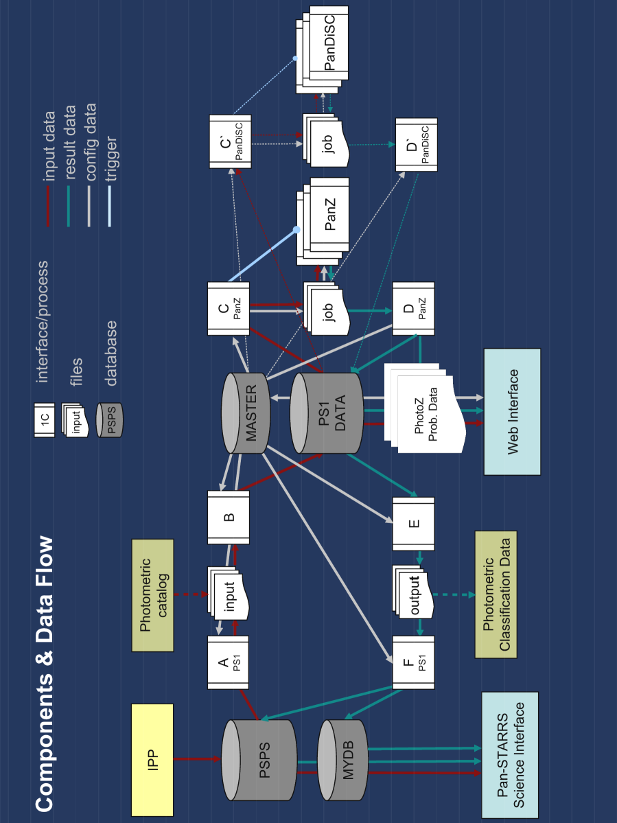
Figure 1: The components of the PCS, see Sect. 5.2 for a description.

5.3 The implementation of PCS

The PCS is implemented on the PanSTARRS cluster, a 175 node (each with 2.6GHz, 4 CPUs and 6 GB memory, for a total of 700 CPUs) Beowulf machine with 180 TB disk space, attached to a PB robotic storing device, mounted at the Max-Planck Rechenzentrum in Garching. The modules described in the previous section are a series of shell scripts, or html/php files, executing php code or SQL commands, or running compiled C++ code. In particular, the input/output interfaces A and F to the PSPS database make use of SOAP/http calls. The Schlegel maps are queried using the routines available from the web. The local database is based on MySQL. A set of Python scripts allows the user to automatically generate plots and statistics similar to Fig. 4 and 5. Presently, new available photometry is downloaded from the PSPS database in chunks of 4 million objects. They are split in blocks of 25000, each of which is sent as a single job to the parallel queue. These numbers are subject to further optimization. The system allows parallel running of jobs operating on the same dataset, but with different recipes.

The performance (in terms of processed objects per second) of the complete system is summarized in the Table 3, where the case of a catalog of 1.8 million objects is presented.

The modular structure of the PCS allows implementation of further components, such as alternative photometric redshift codes and the modules to constrain stellar parameters that are under development.

Table 3: Performance test for the PCS based on a catalog with 1.8 million objects.

Module	Task	Duration	Performance
A	Read from PSPS	4 min	7500/sec
B	File conversion	2:10 min	14000/sec
B	Input data injection	5:20 min	5600/sec
C	Extraction (18 data files)	2:10 min	14000/sec
C	Job creation (18 jobs)	0:30 min	-
PanZ	Running jobs	32 min	950/sec
D	Results injection	16 min	1875/sec
D	PhotoZ-P compression + storage	75 min	400/sec
C′	Extraction (18 data files)	2:00 min	15000/sec
C′	Job creation (18 jobs)	0:30 min	-
PanDiSC	Running jobs	1:00min	30000/sec
D′	Results injection	15 min	2000/sec
E	Results extraction	1:40 min	18000/sec
F	Signal to MyDB	-	-
F	Signal to PSPS	-	-

6 PCS tests

Several spectroscopic surveys overlap with the Pan-STARRS1 MDFs, providing abundant spectral classifications and redshifts: BOSS (Aihara et al., 2011, MDF1, 4, 9, 10), CDFS (Vanzella et al., 2006, MDF2), SDSS and SEGUE/SDSS (Eisenstein et al., 2001; Lee et al., 2008; Abazajian et al., 2009, MDF2 to 10), 2dF Galaxy Redshift Survey (Colless et al., 2001, MDF4), VVDS (Le Févre et al., 2004, 2005; Garilli et al., 2008, MDF1, 7 and 10), ZCosmos (Lilly et al., 2007, MDF4). Here we present tests of PanDiSC and PanZ based on the DR7 SDSS dataset, that provides the largest available homogeneous spectroscopic follow-up of LRGs (selected as DR7 objects with primTarget=32 or 96), the objects for which the Pan-STARRS1 filter set suffices to deliver excellent photometric redshifts. Moreover, the SDSS dataset comprises a large enough sample of stars and QSOs to allow a global sensible test of the capabilities of PCS. The remaining spectroscopic surveys will be discussed in future Pan-STARRS1 papers dealing with the science applications of the PCS.

Table 4 gives the average galactic reddening of the fields covered by SDSS (the largest value of $E(B-V)=0.066$ mag is reached in MDF09) and summarizes the numbers of matched objects, typically several hundreds per field, with more than a thousand in MDF4 and a total of 5784. The same table splits them into stars, galaxies and QSOs. The majority of the matches are galaxies (of which approximately a quarter are red), but numerous (of the order of a hundred) stars and quasars are represented per field. Fig. 2 shows the histograms of the magnitudes in the Pan-STARRS1 filters (within an aperture of 7.4 arcsec radius) for the SDSS spectroscopically classified (and assumed to be the “truth”) stars, galaxies and QSOs of the sample. As expected due to the SDSS spectroscopic limits (resulting from the main spectroscopic sample limited at r=17.77 and the sparser additional surveys, reaching fainter magnitudes), the galaxy sample peaks around $g_{\rm P1}$$\approx 17.5$, while the QSO sample is $\approx 1.5$ mag fainter. The star sample spans a broader range of magnitudes, from $g_{\rm P1}$$\approx 16$ to $\approx 24$. Given the achieved depth of the MDFs, photometric data for this sample has very large signal-to-noise and can be used to test the systematic limitations of PCS. In the following we describe tests performed using both the Pan-STARRS1 and the SDSS photometry, to show that the Pan-STARRS1 dataset is at least as good as SDSS.

Table 4: The SDSS spectroscopic dataset used to test PCS, with number of objects split by star/galaxy/QSO category (LRGs are a subset of galaxies).

MDF	$\langle E(B-V)\rangle$	$N_{SDSS}$	Stars	Galaxies	LRGs	QSOs
	(mag)
3	0.027	704	49	577	107	78
4	0.026	1125	128	880	169	117
5	0.008	913	41	785	155	87
6	0.014	732	27	628	153	77
7	0.011	953	104	755	173	94
8	0.010	226	2	207	49	17
9	0.066	589	54	495	95	40
10	0.038	542	51	436	99	55
Total		5784	456	4763	1000	565

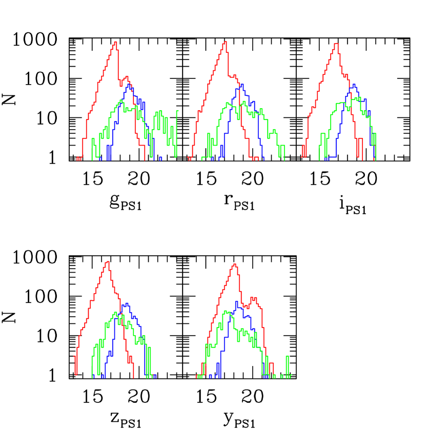
Figure 2: The Pan-STARRS1 magnitude (inside an aperture of 7.4 arcsec radius) histograms matched to the spectroscopic SDSS and classified through the spectroscopic SDSS information as stars (green), galaxies (red) and QSOs (blue).

6.1 Star/Galaxy/Quasar classification

We trained and tested the PanDiSC SVM using a 10-fold cross-validation approach. We divided the sample described in Table 4 with Pan-STARRS1 photometry in 10 partitions, each with 45 stars, 475 galaxies and 55 QSOs. Note that they span the magnitude ranges shown in Fig. 2. We constructed 10 subsets by randomly selecting 55 out of the 475 galaxies. We created 10 training sets, by concatenating 9 of the subsets, and tested the PanDiSC SVM on each of the 10 partitions not used in the 10 training sets.

Table 5 shows the results: galaxies are classified correctly in almost 97% of cases, with very small variations from field to field. Stars (one of which having equal probability of being a star, a galaxy or a QSO, and therefore not considered) and QSOs are recovered on average in $\approx 84$ % of cases. Successful star classification goes up to 95% for MDF5, and is as low as 75% for MDF10. Successful QSO classification is at the 87% level in MDF4 and drops to 69% for MDF9. We will investigate the statistically significance and possible cause of these variations with future larger Pan-STARRS1 catalogs.

The relatively poor performance of the stellar classification is driven by early-type stars alone (correctly classified in 80% of cases) and the Pan-STARRS1 filter set. The classification of late-type stars is better, with just 4% of the late stars being wrongly classified as galaxies.

We now look at the fraction of false positives. Only 21 stars and 44 QSOs are classified as galaxies, therefore the galaxy sample defined by PanDiSC is contaminated at the level of 1%. This is not unexpected, because the extragalactic MDF number counts are dominated by galaxies. The purity of the star and QSOs samples are much worse. There are 38 galaxies and 47 QSOs classified as stars, which results in a 19% contamination of the star catalog defined by PanDiSC. Without the contribution of galaxies, which could be flagged by adding morphological information (i.e. whether the objects are point-like or extended), the contamination (by QSOs) reduces to 10%. Preliminary tests (Klement, 2009) show that this development is indeed very promising. There are 47 stars and 107 galaxies classified as QSOs. This means that the QSO catalog defined by PanDiSC is contaminated at the 28% level, without galaxies just 8.5%. Clearly, the situation will be different at lower galactic latitudes, where stars dominate the number counts at these magnitude limits. Overall, the results are not much worse than those reported by Elting et al. (2008). They can be improved when larger Pan-STARRS1 catalogs will be available, by optimizing the probability thresholds for making a classification decision, since they depend on the relative distribution of stars, galaxies, quasars in the training/test data sets used to make the assessment.

Fig. 3 presents the Pan-STARRS1 color-color plots with the distributions of stars, galaxies and quasars of the spectroscopic SDSS dataset. Objects that are stars according to the spectroscopic SDSS classification are shown on the left diagrams, objects that are galaxies in the central diagrams and objects that are QSOs on the right diagrams. Objects classified correctly by PanDiSC are shown black. Objects wrongly classified as stars by PanDiSC are shown green, wrongly classified as galaxies red, wrongly classified as QSOs in blue. So a red dot on the left column is a star that PanDiSC classified as a galaxy.

Clearly, misclassifications happen in regions of color space where the different types overlap, where only an additional filter (for example the u band) would help discriminate between the populations. In contrast, late-type stars are seldom misclassified thanks to their red colors that divide them well from galaxies and QSOs. Note that the increased scatter in the stellar $g_{\rm P1}$-$r_{\rm P1}$colors at $r_{\rm P1}$-$i_{\rm P1}$$>1.8$ is due to stars near or below the $g_{\rm P1}$ and $r_{\rm P1}$ magnitude limits of Table 2.

We repeated the same tests based on the 10-fold cross-validation technique using the SDSS Petrosian ugriz photometry: the results are presented in Table 6. While the presence of the u band boosts the success rate for QSOs (up to 94%) and stars (up to 92%, with early type stars correctly classified in 90% of the cases) the absence of the y band and the lower quality of the z band penalizes marginally the galaxy classification (down to 95%) and the stellar classification of late star types (classified correctly in 95% of cases). The star false positives are up to 28% (of the total true stars), due to the higher number of misclassified galaxies, but would drop to just the 6% of misclassified QSOs if information about size were added. The QSO false positives, slightly better at the 27%, drop to just 3% without galaxies. The galaxy false positives stay at the 1% level.

Table 5: SVM predictions for evaluation set using Pan-STARRS1 photometry: the confusion matrix (first in absolute numbers, and second in fractions normalized to 1) with true classes in rows.

True classes	$N_{tot}$	Star	Galaxy	Quasar
Star	449	381	21	47
		0.849	0.047	0.104
Galaxy	4750	38	4605	107
		0.008	0.970	0.022
Quasar	550	47	44	459
		0.085	0.080	0.835

Table 6: SVM predictions for evaluation set using the SDSS Petrosian magnitude ugriz photometry: the confusion matrix (first in absolute numbers, and second in fractions normalized to 1) is given as fractions normalized to 1 with true classes in rows.

True classes	$N_{tot}$	Star	Galaxy	Quasar
Star	450	412	23	15
		0.916	0.051	0.033
Galaxy	4750	99	4525	126
		0.021	0.953	0.026
Quasar	550	25	15	510
		0.046	0.027	0.927

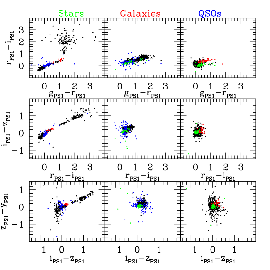
Figure 3: The distribution of SDSS stars (left), galaxies (middle) and QSOs (right) in the color-color plots of Pan-STARRS1. Objects classified correctly by PanDiSC are shown black, objects classified wrongly as stars are green, wrongly as galaxies are red, wrongly as QSO are blue.

6.2 Photometric redshifts

The Pan-STARRS1 photometric dataset misses the u band on the blue side of the spectral energy distribution, and the NIR colors redder than the y band. Therefore one expects any photometric redshift program to perform best for red galaxies at moderate redshifts (e.g., the LRGs), and to fail especially when blue galaxies at low redshifts are considered. Similarly, late stars are expected to be better recognized than earlier ones. Finally, since at present the PhotoZ program misses SEDs optimized for QSOs, we expect poor performances in these cases.

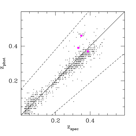
Figure 5: The comparison between spectroscopic and photometric redshifts for the SDSS sample of LRGs. Left: the histogram of $z_{phot}-z_{spec}/(1+z_{spec})$. Right: $z_{spec}$ vs. $z_{phot}$. The magenta points show the three objects for which the QSO SEDs would give the best fit (but a catastrophically poor photometric redshift).

Fig. 4 shows the comparison between spectroscopic and photometric redshifts obtained for the SDSS sample of LRGs, field by field. Fig. 5 shows the results for the whole sample. As usual, we define the percentage of catastrophic failures $\eta$ as the fraction of objects (outliers) for which $|z_{phot}-z_{spec}|>0.15\times(1+z_{spec})$, the residual bias as the mean of $(z_{phot}-z_{spec})/(1+z_{spec})$ without the outliers, and the robust error as $\sigma_{z}=1.48\times Median|z_{phot}-z_{spec}|/(1+z_{spec})$ without the outliers. For LRGs, the Pan-STARRS1 photometry allows the determination of photometric redshifts accurate to 2.4% in $\sigma_{z}$, with bias smaller than 0.5%, no strong trend with redshift and 0.4% catastrophic outliers (when no QSO SED is allowed). No field-to-field dependencies are present.

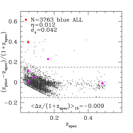
Figure 6: The comparison between spectroscopic and photometric redshifts for the SDSS galaxy sample not classified as LRG. The magenta points show the five of the six objects for which the QSO SEDs would give the best fit (but a catastrophically poor photometric redshift, two of these cases are visible in red).

As expected, the situation is not as satisfactory for non-LRGs. Fig. 6 shows that especially at $z_{spec}<0.2$ the residuals are biased in a systematic way and more than 1% catastrophic outliers are present. Nevertheless, the robust estimate of the scatter remains below 5%.

If we now use for the same galaxies the Petrosian ugriz SDSS photometry, we find the following. The photometric redshifts for LRGs are similarly good (2.6%), but with a higher percentage of outliers. In contrast, precision (3.7%) and percentage of outliers (1%) are better for blue galaxies, where the presence of the u band helps.

As described in Sect. 5.1, PanZ computes also the goodness of fits for a number of stellar templates. Therefore the difference $\chi^{2}_{star}-\chi^{2}_{galaxy}$ between the $\chi^{2}$ of the best-fitting stellar SED $\chi^{2}_{star}$ and the best fitting galaxy SED $\chi^{2}_{galaxy}$ provides a crude galaxy/star classification: if $\chi^{2}_{star}-\chi^{2}_{galaxy}<0$, the stellar template is providing a better fit than the galaxy ones and we classify the object as a star. In Fig. 7, left (where just for plotting convenience we give $\chi^{2}_{star}/\chi^{2}_{galaxy}$) we show that requiring $\chi^{2}_{star}-\chi^{2}_{galaxy}<0$ (i.e. $\chi^{2}_{star}/\chi^{2}_{galaxy}<1$ in the plot) allows to correctly classify spectroscopically confirmed SDSS stars in 73% of the cases. The percentage of successful classifications grows to 89% if only late type SDSS stars are considered. The percentage of success is 98% if spectroscopically confirmed SDSS galaxies are considered (Fig. 7, right).

Finally, we consider the class of QSOs. Fig. 8, left, shows that spectroscopically confirmed SDSS QSOs are classified as QSOs (i.e. are best fit by the QSO SED) in 22% and as galaxies in 50% of the cases. As expected, the photometric redshifts are very poor (Fig. 8, right). The QSO SED in the sample is selected as giving the best-fit in 27% of the cases, giving the right redshift in 20% of the cases. For an additional 28% where catastrophically wrong redshifts are derived, the QSO SED gives the second best fit and a reasonable redshift. Still, if we allow only the QSO SED to be used, we get a good redshift ($\approx 5$% in $\sigma_{z}$) for only 61% of the objects. We are in the process of adding some more QSO SEDs to model better the redshift dependence of QSO evolution. First tests show that only modest improvements can be achieved, since we are hitting the intrinsic limitations of the Pan-STARRS1 filter photometry, combined with the well known difficulties of deriving photometric redshifts for the power-law like, feature-weak shape of QSO SEDs (Budavari et al., 2001; Salvato et al., 2011). The addition of the u band certainly improves the results a lot. When we derive photometric redshifts using the SDSS ugriz Petrosian magnitudes, we get a best-fit with the QSO SED in 51% of the cases (with a photometric redshift good to 5% in 43% of the cases), and for an additional 19% the QSO SED gives the second best solution with the correct redshift. If we allow only the QSO SED to be used, we get a good redshift ($\approx 5$% in $\sigma_{z}$) for 70% of the objects.

Table 7 shows the confusion matrix for PanZ as a Star/QSO/Galaxy photometric classifier. PanZ performs as well as PanDiSC when classifying galaxies, but is poorer when it comes to stars and QSOs, probably due to a lack of appropriate SED templates. As a consequence, the false positive contamination is higher for stars (53%) and galaxies (8%) classes, but lower (4%) for QSOs, compared to PanDiSC. Finally, it is interesting to note that PanZ biases the classification in a different way than PanDiSC: there are 29 stars and 3 QSOs recognized as such by PanZ but not by PanDiSC.

Finally, Table 8 shows the confusion matrix for PanZ as a Star/QSO/Galaxy photometric classifier when the SDSS Petrosian ugriz photometry is used. The percentage of correctly classified QSOs doubles (but is still not competitive with the results of PanDiSC) to reach 44%, the star classification is slightly improved to 80% and the success in the galaxy classification is slightly worse (85%). Therefore, the presence of the u band helps in the classification of (blue) stars and quasars, but does not compensate the absence of the y and of good z band data for galaxies.

As discussed in Sect. 6.1, the final assessment of the relative performances of PanDiSC and PanZ as morphological classifiers will be made when larger Pan-STARRS1 catalogs will allow the derivation of optimal probability thresholds.

Table 7: PanZ as a Star/QSO/Galaxy photometric classifier: the confusion matrix in fractions normalized to 1 with true classes in rows.

True classes	Star	Galaxy	Quasar
Star	0.730	0.241	0.029
Galaxy	0.017	0.981	0.002
QSO	0.285	0.497	0.218

Table 8: PanZ as a Star/QSO/Galaxy photometric classifier using the SDSS Petrosian ugriz photometry: the confusion matrix in fractions normalized to 1 with true classes in rows.

True classes	Star	Galaxy	Quasar
Star	0.797	0.166	0.036
Galaxy	0.131	0.849	0.020
QSO	0.037	0.522	0.441

Figure 4: The comparison between spectroscopic and photometric redshifts for the SDSS sample of LRGs. The difference $(z_{phot}-z_{spec})/(1+z_{spec})$ is shown as a function of $z_{spec}$. The magenta points show the three objects for which the QSO SEDs would give the best fit (but a catastrophically poor photometric redshift).

Figure 7: The efficiency of the PanZ star recognition. Left: for 73% of spectroscopically confirmed SDSS stars PanZ finds a stellar SED as the best fit to the Pan-STARRS1 photometry (i.e. $\chi^{2}_{star}<\chi^{2}_{galaxy}$, note that for plotting convenience $\chi^{2}$ ratios are shown). Of the remaining 123 stars, 13 are best-fit by the QSO SED. Right: PanZ finds $\chi^{2}_{galaxy}<\chi^{2}_{star}$ for 98% of spectroscopically confirmed SDSS galaxies. For 8 of these the QSO SED fits best. For one galaxy the best extragalactic fit is obtained by the QSO SED and is poorer than the one obtained using stellar templates (i.e. $\chi^{2}_{galaxy}>\chi^{2}_{star}$).

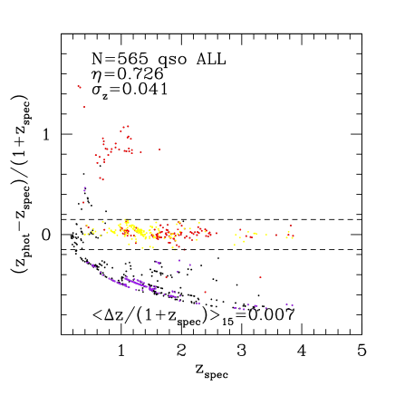
Figure 8: PanZ performances for QSO. Left: for 29% of spectroscopically confirmed SDSS QSOs PanZ finds a stellar SED as the best to the Pan-STARRS1 photometry (i.e. $\chi^{2}_{galaxy}>\chi^{2}_{star}$, note that for plotting convenience $\chi^{2}$ ratios are shown). Right: PanZ redshifts for QSOs. The red dots show the cases where the QSO SED gives the best-fit. The yellow dots show the second-best fit, given by the QSO SED, in cases of catastrophic failures (purple points), where a good redshift is obtained.

7 Conclusions

We presented the Photometric Classification Server of Pan-STARRS1, a database-supported, fully automatised package to classify Pan-STARRS1 objects into stars, galaxies and quasars based on their Pan-STARRS1 colors and compute the photometric redshifts of extragalactic objects. Using the high signal-to-noise photometric catalogs derived for the Pan-STARRS1 Medium-Deep Fields we provide preliminary Star/QSO/Galaxy classifications and demonstrate that excellent photometric redshifts can be derived for the sample of Luminous Red Galaxies. Further tuning of our probabilistic classifier with the large Pan-STARRS1 catalogs available in the future will optimize its already nice performances in terms of completeness and purity. Applied to the photometry that the $3\pi$ survey is going to deliver, possibly combined with u-band or near-infrared photometry coming from other surveys, this will allow us to build up an unprecedented large sample of LRGs with accurate distances. In a future development of PCS we will include size and/or morphological information to improve further the object classification, implement the PanSTeP (Pan-STARRS1 Stellar Parametrizer) software to constrain stellar parameters, and enlarge the SED sample to follow LRGs to higher redshifts and possibly improve results for blue galaxies and QSOs. Alternative photometric redshift codes could also be considered. Moreover, the independent classification information coming from PanZ and PanDiSC will be merged and used to iterate on the photometric redshifts, by narrowing down the choice of SEDs, or deciding which photometry (psf photometry for point-objects versus extended sources photometry for galaxies) is more appropriate for each object.

Facilities: PS1 (GPC1)

References

- Abazajian et al. (2009) Abazajian, K. N. et al. 2009 ApJS, 182, 543.
- Aihara et al. (2011) Aihara, H. et al. 2011, ApJSS, in press
- Adelman-McCarthy et al. (2006) Adelman-McCarthy, K.S.J. et al. 2006, ApJS, 162, 38
- Bailer-Jones et al. (2008) C.A.L. Bailer-Jones, K.W Smith, C. Tiede, R. Sordo, A. Vallenari, 2008, MNRAS 391, 1838
- Bender et al. (2001) Bender, R. et al. 2001, in Deep Fields, edited by S. Cristiani, A. Renzini, and R.E. Williams, Springer-Verlag, Berlin/Heidelberg, p. 96-101
- Bertin & Arnoux (1996) Bertin, E., Arnoux, S. 1996, A&A, 117, 393
- Brimioulle et al. (in prep) Brimioulle, F. et al., in preparation.
- Budavari et al. (2001) Budavari, T., et al. 2001, AJ, 122, 1163
- Chambers et al. (in prep) Chambers, K. C, et al., in preparation.
- Chang & Lin (2011) Chang, C.C., Lin, C.-J. 2011, ACM Transactions on Intelligent Systems and Technology, 2:27:1–27:27
- Colless et al. (2001) Colless, M. et al. 2001, MNRAS, 328, 1039
- Collister & Lahav (2004) Collister, A.A., Lahav, O., PASP, 116, 345
- Csabai et al. (2003) Csabai, I. et al. 2003, AJ, 125, 580
- Dubath et al. (2011) Dubath, P. et al. 2011, MNRAS, 414, 2602
- Eisenstein et al. (2001) Eisenstein D.J. et al. 2001, AJ, 122,2267
- Elting et al. (2008) Elting, C., Bailer-Jones, C.A.L., Smith, K.W., 2008, Ringberg Castle, 14-17 October 2008, Ed. C.A.L. Bailer-Jones, AIP Conference Proceedings vol. 1082, AIP (Melville, New York), p. 9
- Feulner et al. (2005) Feulner, G., et al. 2005, ApJ, 633, L9-L12
- Gabasch et al. (2004) Gabasch, A. et al. 2004, A&A, 421, 41-58
- Gabasch et al. (2008) Gabasch, A. et al. 2008, MNRAS, 383, 1319-1335
- Gao, Zhang & Zhao (2008) Gao, D., Zhang, Y.-X., Zhao, Y.-H. 2008, MNRAS, 386, 1417
- Garilli et al. (2008) Garilli, B. et al. 2008, A&A, 486, 683
- Greisel et al. (in prep) Greisel, N. 2011 et al., in preparation.
- Heasley (2008) Heasley, J.N. 2008, Ringberg Castle, 14-17 October 2008, Ed. C.A.L. Bailer-Jones, AIP Conference Proceedings vol. 1082, AIP (Melville, New York), p. 352-358
- Henrion et al. (2011) Henrion, M., Mortlock, D. J., Hand, D. J. and Gandy, A. 2011, MNRAS, 412, 2286
- Hodapp et al. (2004) Hodapp, K. W., Siegmund, W. A., Kaiser, N., Chambers, K. C., Laux, U., Morgan, J., & Mannery, E. 2004, Proc. SPIE, 5489, 667
- Ilbert et al. (2006) Ilbert, O. et al. 2006, A&A, 457, 841
- Ilbert et al. (2009) Ilbert, O. et al. 2009, ApJ, 690, 1236
- Kaiser et al. (2010) Kaiser, N., et al. 2010, Proc. SPIE, 7733, 12K.
- Klement (2009) Klement, R. J. 2009, PSDC-240-001-00-01, PanStarrs technical note
- Klement et al. (2011) Klement, R. J., Bailer-Jones, C. A. L., Fuchs, B., Rix, H.-W. and Smith, K. W. 2011, ApJ, 726, 103
- Lee et al. (2008) Lee, Y. S., Beers, T. C., Sivarani, T., Allende Prieto, C., Koesterke, L.; Wilhelm, R., Norris, J. E., Bailer-Jones, C. A. L., Re Fiorentin, P., Rockosi, C. M.; Yanny, B., Newberg, H., Covey, K. R. 2008, AJ, 136, 2022
- Lilly et al. (2007) Lilly, S. et al. 2007, ApJS, 172, 70
- Magnier (2006) Magnier, E. 2006, Proceedings of The Advanced Maui Optical and Space Surveillance Technologies Conference, Ed.: S. Ryan, The Maui Economic Development Board, p.E5
- Marengo and Sanchez (2009) Marengo, M. and Sanchez, M. C 2009, AJ, 138, 63
- Mobasher et al. (2007) Mobasher, B. et al. 2007, ApJS, 172, 117
- Magnier (2007) Magnier, E. 2007, The Future of Photometric, Spectrophotometric and Polarimetric Standardization, ASP Conference Series 364, 153
- Magnier et al. (2008) Magnier, E. A., Liu, M., Monet, D. G., & Chambers, K. C. 2008, IAU Symposium, 248, 553
- Magnier et al. (in prep) Magnier, E., et al., in preparation.
- Le Févre et al. (2004) Le Févre, O. et al. 2004, A&A, 428, 1023
- Le Févre et al. (2005) Le Févre, O. et al. 2005, A&A, 439, 845
- Onaka et al. (2008) Onaka, P., Tonry, J. L., Isani, S., Lee, A., Uyeshiro, R., Rae, C., Robertson, L., & Ching, G. 2008, Proc. SPIE, 7014, 12O
- Padmanabhan et al. (2005) Padmanabhan, N. et al. 2005, MNRAS, 359, 237
- Pello et al. (2009) Pello, R. et al. 2009, A&A, 508, 1173
- Platt (1999) Platt, J.C., 1999, Advances in large margin classifiers, Smola, A.J. Bartlett, P., Schoelkopf, D.S. Eds., MIT press
- Richards et al. (2002) Richards, G.T. et al. 2002, AJ, 123, 2945
- Richards et al. (2009a) Richards, G.T. et al. 2009, ApJS, 180, 67
- Richards et al. (2009b) Richards, G.T. et al. 2009, AJ, 137, 3884
- Saglia (2008) Saglia, R.P. 2008, Ringberg Castle, 14-17 October 2008, Ed. C.A.L. Bailer-Jones, AIP Conference Proceedings vol. 1082, AIP (Melville, New York), p. 366
- Saglia et al. (2011) Saglia, R.P., Snigula, J., Senger, R., Bender, R., 2011, Exp.Ast., in press
- Salvato et al. (2011) Salvato, M., Ilbert, O., Hasinger, G. et al. 2011, ApJ, in press
- Schlegel et al. (1998) Schlegel, D.J., Finkbeiner, D.P., Davis, M., 1998, ApJ, 500, 525
- Schmidt et al. (2010) Schmidt, K. B., Marshall, P. J.,Rix, H.-W., Jester, S., Hennawi, J. F., and Dobler, G. 2010, ApJ, 714, 1194
- Smith (2009) Smith, K.W. 2009, GAIA-C8-TN-MPIA-KS-016, GAIA technical note, available at http://www.mpia.de/GAIA/Publications.htm
- Smith et al. (2010) Smith, K. W., Bailer-Jones, C. A. L., Klement, R. J. and Xue, X. X. 2010, A&A, 522, 88
- Snigula et al. (2009) Snigula, J.M., Bender, R. Saglia, R., Drory, N. 2009,ASP Conference Series, J. Lewis, R. Argyle, P. Bunclarck, D. Evans, E. Gonzales-Solares Eds., 421, 268-271
- Stubbs et al. (2010) Stubbs, C. W., Doherty, P., Cramer, C., Narayan, G., Brown, Y. J., Lykke, K. R., Woodward, J. T., & Tonry, J. L. 2010, ApJS, 191, 376
- Telfer et al. (2002) Telfer, R. C.; Zheng, W., Kriss, G. A.; Davidsen, A. F. 2002, ApJ, 565, 773
- Tonry & Onaka (2009) Tonry, J., & Onaka, P. 2009, Advanced Maui Optical and Space Surveillance Technologies Conference, Proceedings of the Advanced Maui Optical and Space Surveillance Technologies Conference, Ed.: S. Ryan, p.E40.
- Tonry et al. (in prep) Tonry, J. L., et al., in preparation.
- Tzalmantza et al. (2007) Tsalmantza, P. et al. 2007, A&A, 470, 761
- Tzalmantza et al. (2009) Tsalmantza, P. et al. 2009, A&A, 504, 1071
- Valentijn et al. (2006) Valentijn, E.A., Begeman, K.G., Boxhoorn, D.R. et al. 2006, in “Astronomical data analysis software and systems XVI, R. Shaw, F. Hill and D. Bell Eds., ASP, R. Shaw, F. Hill and D. Bell Eds., 376, 491-498
- Vander Berk et al. (2001) Vanden Berk, D.E. et al. 2001, AJ, 122, 5490
- Vanzella et al. (2006) Vanzella, E. et al. 2006, A&A, 454, 423
- Vasconcellos et al. (2011) Vasconcellos, E.C. et al. 2011, AJ, 141, 189
- York et al. (2000) York, D.G. et al. 2000, AJ, 120, 1579
- Wu, Lin & Weng (2004) Wu, T.-F., Lin, C.-J., Weng, R.C., Journal of Machine Learning Research, 5, 975