COSMIC ACCELERATION AND A NEW CONCORDANCE FROM CAUSAL BACKREACTION

Abstract

A phenomenological formalism is presented in which the apparent acceleration of the universe is generated by large-scale structure formation, thus eliminating the magnitude and coincidence fine-tuning problems of the Cosmological Constant in the Concordance Model, as well as potential instability issues with dynamical Dark Energy. The observed acceleration results from the combined effect of innumerable local perturbations due to individually virializing systems, overlapping together in a smoothly-inhomogeneous adjustment of the FRW metric, in a process governed by the causal flow of inhomogeneity information outward from each clumped system. After explaining why arguments from the literature claiming to place restrictive limits upon backreaction are not applicable in a physically realistic cosmological analysis, we present a selection of simply-parameterized models which are capable of fitting the luminosity distance data from Type Ia supernovae essentially as well as the best-fit flat $\Lambda$CDM model, without resort to Dark Energy, any modification to gravity, or a local void. Simultaneously, these models can reproduce measured cosmological parameters such as the age of the universe, the matter density required for spatial flatness, the present-day deceleration parameter, and the angular scale of the Cosmic Microwave Background to within a reasonable proximity of their Concordance values. A potential observational signature for distinguishing this cosmological formalism from $\Lambda$CDM may be a cosmic jerk parameter significantly in excess of unity.

1 INTRODUCTION AND MOTIVATIONS

Evidence from the past decade or so indicating that we live in a spatially flat (Larson et al., 2011), accelerating (Perlmutter et al., 1999; Riess et al., 1998) universe, yet one in which the density of clustering matter is significantly less than the critical density (e.g., Turner, 2002), has led cosmologists to a surprising conclusion: the dominant cosmic component appears to be “Dark Energy”, a smoothly-distributed material that must possess negative pressure in order to be able to drive the acceleration (e.g., Kolb & Turner, 1990).

The true nature of this Dark Energy remains very much in doubt, however. The simplest version, a Cosmological Constant ($\Lambda$), suffers from well-known aesthetic difficulties, including two different fine-tuning problems: one being the issue that $\rho_{\Lambda}$ is $\sim$$120$ orders of magnitude smaller than what would be expected from the Planck scale (e.g., Kolb & Turner, 1990); and the other being a “Coincidence Problem” (e.g., Arkani-Hamed et al., 2000) which questions why, given $\rho_{\Lambda}/\rho_{\mathrm{M}}\propto a^{3}$, that observers today should just happen to live right around the time (within a factor of $\sim$$2$ in scale factor) when $\Lambda$ began dominating the cosmic evolution.

One possible way of ameliorating such problems is to give the Dark Energy an evolving equation of state, $w(z)$, where such coincidences are eliminated or moderated (like in tracker quintessence; e.g., Zlatev et al. (1999)). But moving away from a Cosmological Constant by giving the Dark Energy an evolution in $w(z)$ also opens the door to other possible dynamics – such as the ability for the Dark Energy to be mobile and thus perhaps to become spatially inhomogeneous (Caldwell et al., 1998). A dynamical Dark Energy (DDE) of this type is liable to join in structure formation to an observationally unacceptable degree, thus ruining it as a candidate to serve as the “smoothly-distributed” missing cosmic ingredient.

From the $1^{\mathrm{st}}$ Law of Thermodynamics, $\mathrm{Pressure}=-\partial[\mathrm{Energy}]/\partial[\mathrm{Volume}]$, so that a ‘negative pressure’ ($P<0$) substance like Dark Energy will have $\partial E/\partial V>0$; consequently, it should be self-attractive on local scales (and relativistically so, since $w\equiv P/\rho\sim-1$), in stark contrast to how Dark Energy is popularly described as a “repulsive” or “antigravity” material (e.g., Heavens, 2010). This potential instability of DDE to spatial perturbations must be countered through the addition of some nonadiabatic support pressure (an adiabatic positive pressure term would cause cosmic deceleration); and though this can apparently be done (e.g., Caldwell et al., 1998; Hu, 2005), other results exist (Maor & Lahav, 2005) indicating that a Dark Energy allowed to dynamically participate in virialization does indeed show signs of providing an additional attractive force for clustering, rather than opposing clustering or leaving it unaffected. In any case, an inhomogeneous DDE supported against extensive clumping by nonadiabatic pressure would not be a perfect fluid, and since a perfect fluid approximation is the basis of the argument for acceleration ($\ddot{a}>0$) from $P<0$ (e.g., Kolb & Turner, 1990, pp. 48-50), the entire situation is best avoided if possible.

Interestingly, the self-attractive nature of negative pressure presents us with the seed of an alternative idea: in its own way, normal gravitational attraction represents a form of ‘negative pressure’ – in particular, the gravitational attraction responsible for the growth of clustering in large-scale structure formation. Making a virtue of necessity, one may therefore recruit cosmic structure formation as the driver (not just the trigger, as in tracker quintessence) of the cosmic acceleration. This would completely solve the Coincidence Problem, since the remarkably contemporary onsets of both the acceleration and the existence of galaxies (and hence planets, life, and astronomical observers) would be nothing more coincidental than finding two neighboring apples that have fallen from the same tree.

Such considerations are what initially led this author to search for a structure-formation-induced solution to the cosmic acceleration problem (Bochner, 2007), though a plausible acceleration mechanism was not yet apparent. During the past few years, a number of other researchers have similarly proposed a variety of methods (e.g., Schwarz, 2002; Räsänen, 2004; Kolb et al., 2005; Wiltshire, 2007, as a few examples) also attempting to obtain the observed cosmic acceleration from the breaking of FLRW homogeneity and the formation of structure, without requiring the intervention of non-standard gravitational or particle physics, or the non-Copernican approach of placing us near the center of a large cosmic void. This type of approach has become generally known as “backreaction”. The backreaction paradigm, in the consensus view, has been unable to substantially replace Dark Energy as the source of the apparent acceleration; a conclusion which we will argue is quite premature.

In this paper, in fact, we will present a physically plausible (though phenomenological) mechanism that is not only able to reproduce the cosmic acceleration as indicated by observations of standard candles such as Type Ia supernovae, but which can also reproduce several other key features of the conventional $\Lambda$CDM concordance.

The paper will be organized as follows: in Section 2, we explain why several oft-quoted limitations of the backreaction mechanism are inapplicable in realistic situations, and then use such arguments as guideposts towards developing our formalism in Section 3; in Section 4, we describe our specific models and present our simulated Hubble curves; in Section 5, we evaluate the success of our models in formulating an alternative “Cosmic Concordance”; and we conclude in Section 6. Note that the in-depth technical details of the research introduced here are discussed much more fully in a companion paper by this author (Bochner, 2011).

2 THE COSMOLOGICAL IMPACT OF “BACKREACTION”

At present, backreaction is not widely considered to be a viable method for achieving the observed acceleration (e.g., Schwarz, 2010). There are a number of important reasons for this view, reasons which seem on the surface to be strong arguments; but we will explain here why despite being technically correct, several of those arguments do not properly apply to a physically realistic cosmological model.

One popular approach for estimating (and placing limits upon) the effects of backreaction is to use “Swiss-Cheese” solutions – regular FLRW cosmologies with spherical ‘holes’ cut out of them, with precisely designed boundary conditions so that the exterior universe (the ‘cheese’) remains completely unaffected by the holes. Such models are advantageous because exact solutions may be used for the clumped material inside the holes, allowing for a precise analysis. But the weakness of such models is their significant lack of realism: not only do most of them lack any mechanism for representing structure virialization and stabilization, but they have in fact been specially designed to set the actual backreaction (as opposed to purely observational effects) to zero, by hermetically sealing off each condensed structure so that it cannot affect the exterior universe (even shielding the holes from one another). In the real universe, though, the ‘spheres of influence’ of individual mass overdensities continually expand over time, affecting more and more distant objects, until multiple ‘independent’ influences eventually overlap and merge. This superposition of gravitational perturbations from many different inhomogeneities is a phenomenon that Swiss-Cheese models cannot represent at all. Thus we understand why Swiss-Cheese backreaction calculations fail to find effects strong enough to produce the observed acceleration – such as, for example, the findings of Biswas & Notari (2008) showing that the perturbative effects of a hole on observations are strongly suppressed, by a factor $(L/R_{H})^{3}$ for passage through the hole, where $L$ is the size of the hole and $R_{H}$ is the Hubble radius. Recognizing the improperly artificial act of abruptly cutting off the gravitational influence of an overdensity at hole ‘edge’ $r=L$, as the Swiss-Cheese models do, we see therefore that the smallness of the suppressive term $(L/R_{H})^{3}$ is itself completely artificial. A realistic backreaction model would not have any predetermined limits on $L$, but rather would allow it to grow without bound (within causal speed limits for the propagation of gravitational perturbation information), overlapping with more and more distant holes, until the factor $(L/R_{H})^{3}$ is no longer much of a ‘suppression’, after all.

Another argument claiming to limit the efficacy of backreaction is the acceleration “no-go” theorem of Hirata & Seljak (2005), based upon the Raychaudhuri equation (Hawking & Ellis, 1973), demonstrating that a ‘true’ (volumetric) acceleration of a spatial region is impossible in the absence of a material with sufficiently negative pressure ($w<-1/3$) to serve as Dark Energy. This conclusion only holds, however, as long as one assumes the cosmic matter to be irrotational – that is, possessing zero vorticity. But here we must ask: Why is the vorticity set to zero? This seems to be an especially unusual prescription in a universe where nearly everything is rotating or revolving about something. Essentially all virialized structures in the universe larger than individual solid objects are stabilized against collapse by some version of vorticity or velocity dispersion; and it is certainly a bad physical approximation to take the dominant physical force (in opposition to gravity) which regulates cosmic structure formation, and completely set it to zero. Since vorticity in significant amounts – on large scales, at least – is not a prediction of inflation (Hirata & Seljak, 2005), it is typically regarded as a “small-scale player” (e.g., Buchert, 2008), relevant only for cosmic averages performed over domains that are on or below the scales of galaxy clusters; and thus it is usually set to zero for technical convenience (e.g., Räsänen, 2010), a seemingly harmless simplification. But this ignores the fact that the term actually appearing in the Raychaudhuri equation is not the vorticity tensor $\omega_{\mu\nu}$, but the square of the vorticity, $\omega^{2}$, a quantity that will never average away. As Buchert & Ehlers (1997) put it, cosmic averages of positive semi-definite quantities like $\langle\omega^{2}\rangle$ get “frozen” at the size of “typical subdomains”; and thus they cannot be made to go to zero by averaging over larger domains, even if the spatially-averaged value of the parent tensor, $\langle\omega_{\mu\nu}\rangle$, does itself become negligible on large scales. Thus dropping vorticity entirely from the cosmic evolution is a very poor approximation.

We do not attempt here to explicitly model the enormously complex backreaction effects of vorticity during the dynamical virialization of a structure; rather, we exploit the very simple natures of both the beginning state (nearly perfectly smooth FRW matter), and the ending state (reasonably randomly distributed Newtonian mass concentrations) of structure formation. This will lead (in Section 3, below) to a phenomenological formalism depending only upon the general evolution rate of the cosmic matter from “smoothness” to “clumpiness” over time.

Lastly, note that our formalism uses the backreaction effects of Newtonian-strength (i.e., gravitationally linear) perturbations, despite the extensive work of Buchert and collaborators (e.g., Buchert & Ehlers, 1997) seemingly demonstrating that the entire Newtonian-level backreaction can be expressed mathematically as a total divergence, thus guaranteeing it to be either extremely small or identically zero (depending upon the boundary conditions). But comparing Equations 1a–d of Buchert & Ehlers (1997) to Maxwell’s Equations (e.g., Jackson, 1975) shows that their formalism contains a crucial simplification: a dropping of all “gravitomagnetic” fields from their calculations. Similar to how structure formation calculations are based upon the Poisson equation, $\nabla^{2}\Phi=4\pi G\rho$ (though suitably modified for the cosmic expansion), in which the time-derivative terms of the full wave equation have been dropped, this is an explicitly non-causal formalism. (Other backreaction no-go arguments like that in Ishibashi & Wald (2006) are also reliant upon dropping terms like $|\partial\Phi/\partial t|^{2}$, as seen via their Equation 2b.) This simplification is typically justified by citing the smallness of $v^{2}/c^{2}$ given the (reasonable) assumption of nonrelativistic speeds for most matter flows; but there is a crucial difference between “small” and “suppressed”. Many individually small contributions can be added together to produce a large overall result, if one has enough of them; and though Newtonian-level perturbations weaken as $\sim$$1/r$, the number of them in a spherical shell increases as $\sim$$r^{2}$ (easily overwhelming any factors of $v^{2}/c^{2}$), creating a total perturbative effect that would formally be infinite when integrated out to $r=\infty$, if not reined in by the finite causal horizon out to which an observer can ‘see’ clumped structure that has had sufficient time since the Big Bang to form; a situation reminiscent of Olbers’ Paradox (Weinberg, 1972).

For a causality-respecting approach, one must instead (as in electrodynamics) use the full wave equation, for special-relativistically consistent perturbation potential function $\Phi_{\mathrm{SR}}$:

$$\nabla^{2}\Phi_{\mathrm{SR}}-\frac{1}{c^{2}}\frac{\partial^{2}\Phi_{\mathrm{SR}}}{\partial t^{2}}=4\pi G\rho~{}.$$ (1)

(Note that factors relating to the cosmic expansion are still neglected here, for simplicity.) Now, the usual impulse is to immediately drop the extra term in Equation 1, involving $\partial^{2}\Phi_{\mathrm{SR}}/\partial t^{2}$ – equivalent to dropping the gravitomagnetic terms, as is done in the Buchert formalism – because of its resulting prefactor of $v^{2}/c^{2}$; this factor would seem to make it very small given the assumption of nonrelativistic speeds for most matter flows, and thus (assumedly) ensuring it to be negligible compared to the spatial variations term in any backreaction calculation. But this thinking is based only upon considerations of individual Fourier perturbation modes, not on the overall causal behavior of information flow in the structure-forming universe. If we instead keep all terms, and solve Equation 1 as-is, then one gets (adapting from Jackson, 1975, eq. 6.69):

$$\Phi_{\mathrm{SR}}({\bf x},t)=-G\int^{\infty}\frac{[\rho({\bf x^{\prime}},t)]_{\mathrm{ret}}}{|{\bf x}-{\bf x}^{\prime}|}d^{3}x^{\prime}~{},$$ (2)

where the bracketed numerator is always evaluated at the retarded time, $t^{\prime}=t-|{\bf x}-{\bf x}^{\prime}|/c$. It is this retarded-time condition which restores causality, allowing different regions of the universe to communicate with (and gravitationally perturb) one another; and which provides the escape route from the Buchert suppression of Newtonian-level backreaction, because such backreaction is not truly expressible as a total divergence. We will refer to this propagation of gravitational perturbation information between distant (though communicating) regions as “causal updating”.

Given the fact that the key metric perturbation function, $\Phi_{\mathrm{SR}}(t)$, is predominantly affected by inhomogeneity information coming in from distant locations, the retarded-time condition of an integrated formula like Equation 2 (suitably modified for cosmological calculations) implicitly gives it the ability to exhibit relativistic behavior in what would otherwise appear to be nonrelativistic situations. Consider the farthest distance (at some given observation time, $t$) out to which the look-back time still represents a fairly clumpy universe; this distance (as a function of $t$) represents the edge of an outgoing “wave of observed clumpiness” expanding outward from an observer at $c$, which ensures that the potential function $\Phi_{\mathrm{SR}}$ for perturbations felt by that observer will be fully (special-)relativistic in character, even if none of the matter in the universe is actually moving at relativistic speeds. This unexpected result is due to the fact that cosmological systems (unlike anything else) are infinite in size, meaning that the inherently relativistic act of causal observation will end up encompassing spatial volumes which are incomparably vast, causing even small effects to sum together to produce a dominant overall influence. Perhaps surprisingly, therefore, the apparent acceleration of the universe which we observe is not caused by any individually powerful or gravitationally exceptional specific objects or regions, but rather is an effect that comes from the summed influences of the weak-gravity Newtonian tails of innumerable mass concentrations, imposing their combined effects upon us from extraordinarily large distances.

In this approach, it is clear that we are advocating a diametrically-opposed view from that of other authors who have sought to define a “finite infinity” (e.g., Cox, 2007), representing a very limited boundary from within which significant effects upon some specified local volume can have ever arrived. Such a limitation would restrict the history of ‘important’ interactions to be within an effective “matter horizon” (Ellis & Stoeger, 2009) of only a few Mpc in size, delineated by the timelike world lines traveled by pressure-free matter due to scalar perturbations. But interestingly, both Cox (2007) and Ellis & Stoeger (2009) acknowledge the Great Attractor/Shapley Concentration as a likely source of our bulk flow – i.e., as the completely dominant influence upon the motion of our entire neighborhood of galaxy clusters – despite the clearly contradictory fact (for their claims) that those structures which control our bulk motion are exceedingly far beyond any reasonable estimate of our so-called matter horizon. Thus one cannot take at face value the assertion in Ellis & Stoeger (2009) that, “the strengths of any other possible long distance influences… gravitational waves, or electric Weyl tensor components from sources outside that region – are insignificant compared to local effects.” Notably, it has been shown by Ludvigsen (1989) that even an arbitrarily small energy flux due to gravitational waves can result in a finite amount of “geodesic deviation” (actually, long-term positional displacements of observers due to permanent metric changes) in the very distant radiation zone.

Nevertheless, there are very straightforward calculations using gravitational perturbation theory which are commonly believed to contradict any assertions of the significance of such nonlocally-acting causal backreaction effects. The problem, however, is the fact that perturbation theory is singularly ill-equipped for dealing with the most important perturbative effects in an unbounded system like the (effectively) infinite universe. The central difficulty with perturbation theory here relates to its basic program of identifying the ‘important’ physics by labeling the amplitude of each term as “large” or “small”, and then dropping the small terms in order to focus upon the large ones. For example, Kolb et al. (2005) neglect information-carrying tensor modes generated by nonlinear scalar perturbations (i.e., virializing masses) in the final expressions for their analysis (as well as assuming irrotational dust, thus neglecting vorticity). In a similar vein, both Räsänen (2012) and Gromes (2011) assume that time derivatives of metric perturbations are small, leading to the conclusion that velocity-dependent terms can safely be neglected; and Gromes (2011) specifically uses this point as a primary argument for dismissing the effects of causal backreaction entirely. Obviously, though, if one removes all “causal” aspects from “causal backreaction”, then nothing will be left, and it is unsurprising for one to then find that backreaction fails to work, given that the principal physics responsible for it has been intentionally set to zero. But this basic procedure is conceptually flawed in the case of causal backreaction, which deals with propagating modes, since such modes can bring in gravitational perturbation information to a local observer from vast spatial volumes, so that a term with a ‘small amplitude’ can actually produce an enormous overall effect.

The habit of conflating “small” with “negligible” is a continuing error in perturbation theory analyses of cosmological evolution, since the size of these effects, in terms of amplitude, effectively does not matter: it is practically irrelevant how small the time-derivative terms may be, when one realizes that such effects are being cumulatively contributed by all of the matter within a causal horizon that may be billions of light-years in extent, thus multiplying that amplitude by an amount of mass easily large enough to overcome its inherent smallness. Furthermore, even if the amplitudes of the relevant perturbative terms for causal backreaction were somehow ‘magically’ made even smaller than they naturally are, this still would not shut off the causal backreaction effect, but merely postpone it to begin a little bit later, since a somewhat larger causal horizon of self-stabilizing inhomogeneities would then be needed to supply a large enough integrated effect to cause an apparent acceleration. In that sense, one could never make the amplitudes of those perturbation terms small enough to avoid the eventual dominance of causal backreaction, since a big enough causal horizon (containing a sufficiently large amount of virializing mass) can always be attained after a sufficiently long period of time, which when multiplied by even the smallest amplitude, would eventually produce a term of order unity that then proceeds to dominate the cosmic evolution. Thus for causal backreaction in an effectively infinite universe, there is no such thing as “negligible”.

3 THE PHENOMENOLOGICAL FORMALISM OF CAUSAL BACKREACTION

We require a practical way to implement these ideas, so consider the following. It is well known (Weinberg, 1972, pp. 474-475) that the Friedmann expansion for some spherical volume $\mathbf{V}$ can be derived – using nonrelativistic Newtonian equations, in fact – without reference to anything outside of that sphere. In a sense, the outside universe might as well not even exist for $\mathbf{V}$, in a completely smooth cosmology.

This changes when perturbations develop, however, since clumped structures external to $\mathbf{V}$ exert measurable gravitational forces upon the mass within it; and such forces are new, as if those clumped structures were brought in from infinity at some recent time during the structure formation epoch, to only then begin affecting $\mathbf{V}$. But one cannot feel a gravitational force, unless one simultaneously feels a gravitational potential; and so the perturbing potential within $\mathbf{V}$ must also be new in every physically measurable sense as well, approaching and entering $\mathbf{V}$ in causal fashion from some clumped object (and from all others) as they develop over time, everywhere in the surrounding universe.

For a randomly-distributed collection of inhomogeneities, the forces exerted upon the mass in $\mathbf{V}$ would pull in all directions, largely canceling one another; and indeed, our formalism is based upon a “smoothly-inhomogeneous” universe for which spatial variations are essentially averaged out. But what does not cancel out, regardless of how the perturbations outside of $\mathbf{V}$ are distributed – because it is a non-directional scalar, rather than a vector – is their combined contribution to the absolute level of the potential $\Phi$, which may not matter in true Newtonian physics (only potential differences or gradients do), but which does matter in general relativity. This overall perturbation potential $\Phi_{\mathrm{SR}}(t)$ is treated here as independent of position; but it fully obeys causality, growing as perturbation information comes in from the limits of one’s observational horizon. Our phenomenological approach thus models the inhomogeneity-perturbed evolution of (any volume) $\mathbf{V}$ with a metric that contains the individual Newtonian-level perturbations from all clumped, virialized structures that have been causally ‘seen’ within $\mathbf{V}$ by time $t$, superposed on top of its (internally-generated) background Friedmann expansion.

This is clearly a very heuristic picture, with the growing perturbation potential $\Phi_{\mathrm{SR}}(t)$ not representing the literal metric of the universe, but rather acting as a quantifiable shorthand for the dominant backreaction effects from structure formation. What is really happening, is that virializing overdensities halt their collapse by concentrating their local vorticity (and/or velocity dispersion); this concentrated vorticity leads to real, extra volume expansion, representable (in the final state) at great distances by the tail of a Newtonian perturbation potential to the background FRW metric; this Newtonian tail propagates outward into space by inducing inward mass flows towards the virialized object from farther and farther distances as time passes; and the total perturbation at any given location will be the combined effects of innumerable Newtonian tails of this type, coming in causally (from all directions) from within that location’s ever-expanding “inhomogeneity horizon”. Our formalism merely uses $\Phi_{\mathrm{SR}}(t)$ to represent all of these complex physical processes in a very simple way, and we will see that this is sufficient for producing an observed acceleration fully in agreement with observations.

To phenomenologically model the cosmological phase transition from the extremely symmetrical and smooth (“unclumped”) state during the early universe, to its almost entirely “clumped” state today, we employ a “clumping evolution function”, $\Psi(t)$, defined over the range from $\Psi(t)=0$ (perfectly smooth matter) to $\Psi(t)=1$ (everything clumped). Note that we assume a spatially flat background – for the pre-perturbed universe – everywhere in our calculations, and that we therefore assume the entire universe to be composed of pressureless dust with $\Omega^{\mathrm{FRW}}_{\mathrm{M}}\equiv 1\neq\Omega^{\mathrm{Obs}}_{\mathrm{M}}$ (the superscript “Obs” referring to observational quantities).

The Newtonian approximation for a single clumped object of mass $M$ (representing a virialized, self-stabilized inhomogeneity), embedded at the origin ($r=0$) in an expanding, spatially flat, matter-dominated (MD) universe can be obtained by linearizing the McVittie solution (McVittie, 1933), as can be seen from the perturbed FRW expression given in Kaloper et al. (2010). One gets:

$$ds^{2}\approx-c^{2}[1+(2/c^{2})\Phi(t)]dt^{2}+[a_{\mathrm{MD}}(t)]^{2}[1-(2/c^{2})\Phi(t)]dr^{2}+[a_{\mathrm{MD}}(t)]^{2}r^{2}[d{\theta}^{2}+\sin^{2}{\theta}d{\phi}^{2}]~{},$$ (3)

where $\Phi(t)\equiv\{-GM/[a_{\mathrm{MD}}(t)r]\}$, and $a_{\mathrm{MD}}(t)\propto t^{2/3}$ is the unperturbed MD scale factor.

Assuming that such mass concentrations will be randomly and (sufficiently) evenly distributed throughout the universe, one must integrate over distance (from a particular observer’s location) for the various clumps, and one must also angle-average over them to get the metric for the combined effects that would represent an averaged $ds^{2}$ typical for that observer experiencing displacements in any given direction. Since a displacement of magnitude $|d\vec{r}|$ will have a radial component (with respect to any particular mass concentration) of $|d\vec{r}|\cos\theta$, angle-averaging thus brings in a factor of $\langle\cos^{2}\theta\rangle=(1/3)$ for the spatial part of the metric perturbation term, while leaving its temporal part unchanged.

Consider now the observer to be located at the origin, surrounded by a set of (roughly identical) discrete mass concentrations with total mass $M$, all located within a particular spherical shell at coordinate distance $r^{\prime}$ from the origin, but randomly distributed in $(\theta,\phi)$. From the above arguments, we can write the total, linearly summed and angle-averaged metric in ‘isotropized’ fashion, as:

$$ds^{2}=-c^{2}\{1-[R_{\mathrm{Sch}}(t)/r^{\prime}]\}~{}dt^{2}~{}+~{}[a_{\mathrm{MD}}(t)]^{2}\{1+(1/3)[R_{\mathrm{Sch}}(t)/r^{\prime}]\}~{}|d\vec{r}|^{2}~{},$$ (4)

where $R_{\mathrm{Sch}}(t)\equiv\{(2GM/c^{2})/[a_{\mathrm{MD}}(t)]\}$, and $|d\vec{r}|^{2}\equiv(dr^{2}+r^{2}d\theta^{2}+r^{2}\sin^{2}{\theta}d\phi^{2})=|d\vec{x}|^{2}\equiv(dx^{2}+dy^{2}+dz^{2})$. Regarding the spatial metric perturbation term as a ‘true’ increase in spatial volume, and the perturbation in $g_{tt}$ as an ‘observational’ slowdown of the perceptions of observers (relative to the expansion governed by cosmic time $t$), we see that even if the spatial term by itself is not enough to generate a real volumetric acceleration, when coupled with the temporal term the entire perturbation may indeed be enough to create a so-called “apparent acceleration” sufficient to explain all of the relevant cosmological observations.

The expression in Equation 4 represents the perturbations to the metric due to masses at some specific coordinate distance $r^{\prime}$ – and thus from a specific look-back time $t^{\prime}$ – as seen from some particular observational point. The total metric at that spacetime point must be computed via an integration over all possible distances, out to the distance (and thus look-back time) at which the universe had been essentially unclustered. Finally, a light ray reaching us from its source (e.g., a Type Ia supernova being used as a standard candle) travels to us in a path composed of a collection of such points, where the metric at each point must be calculated via its own integration out to its individual “inhomogeneity horizon”; and only by calculating the metric at every point in the pathway from the supernova to our final location here at $r=z=0$ can we figure out the total distance that the light ray has been able to travel through the increasingly perturbed metric, given its emission at some specific redshift $z$.

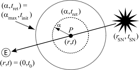
Figure 1: Geometry for computing the inhomogeneity-perturbed metric at each point along the integrated path of a light ray from a supernova to our observation point at Earth.

Consider a light ray emitted by a supernova at cosmic coordinate time $t=t_{\mathrm{SN}}$, which then propagates from the supernova at $r=r_{\mathrm{SN}}$, to us at $r=0$, $t=t_{0}$. We refer here to the geometry depicted in Figure 1.

For each point $P\equiv(r,t)$ of the trajectory, the metric at that point will be perturbed away from the background FRW form by all of the virialized clumps that have entered its causal horizon by that time. Consider a sphere of (coordinate) radius $\alpha$, centered around point $P$, with coordinates $(\alpha,t_{\mathrm{ret}})$ (where $t_{\mathrm{ret}}\leq t$ is the retarded time), defined such that the information about the state of the clumping of matter on that sphere at time $t_{\mathrm{ret}}$ will arrive – via causal updating, traveling at the speed of null rays – to point $P$ at the precise time $t$. To compute the fully-perturbed metric at $P$, we must integrate over the clumping effects of all such radii $\alpha$, from $\alpha=0$ out to $\alpha_{\mathrm{max}}$, the farthest distance from $P$ out from which clumping information can have causally arrived since the clustering of matter had originally begun in cosmic history.

The full derivations of all formulae shown below are given in Bochner (2011); here we quote the resulting equations, which are used for our causal backreaction simulations.

For a FRW metric with $a(t)=a_{\mathrm{MD}}(t)\equiv a_{0}(t/t_{0})^{2/3}\equiv c[18t^{2}/H_{0}]^{1/3}$, the retarded time $t_{\mathrm{ret}}$ can be given as:

$$t_{\mathrm{ret}}(t,\alpha)=t_{0}[(t/t_{0})^{1/3}-\alpha]^{3}~{}.$$ (5)

Similarly, we can determine $\alpha_{\mathrm{max}}$, given some initial time $t_{\mathrm{init}}$ at which structure formation can be reasonably said to have started (i.e., $\Psi(t\leq t_{\mathrm{init}})\equiv 0$):

$$\alpha_{\mathrm{max}}(t,t_{\mathrm{init}})=[(t/t_{0})^{1/3}-(t_{\mathrm{init}}/t_{0})^{1/3}]~{}.$$ (6)

Now, how the metric is affected at $P$ by a spherical shell of material at coordinate radius $\alpha$ depends upon the state of clumping there at the appropriate retarded time: $\Psi[t_{\mathrm{ret}}(t,\alpha)]$. The total effect is computed by integrating all shells from $\alpha=0$ out to $\alpha=\alpha_{\mathrm{max}}(t,t_{\mathrm{init}})$; but in order to compute the metric perturbation from each shell quantitatively, it is first necessary to relate this clumping function to an actual physical density of material.

Recalling Equation 4, we have the perturbation term $[R_{\mathrm{Sch}}(t)/r^{\prime}]=\{(2GM/c^{2})/[r^{\prime}~{}a_{\mathrm{MD}}(t)]\}$, where the value of $M$ to use here at time $t$ is given by the clumped matter density, $[\Psi(t)\rho_{\mathrm{crit}}(t)]$, times the infinitesimal volume element of the shell. Collecting all relevant factors (and letting $t^{\prime}\equiv t_{\mathrm{ret}}(t,\alpha)$), the integrand at coordinate distance $\alpha$ can eventually be written as:

$$[R_{\mathrm{Sch}}(t)/r^{\prime}]_{r^{\prime}=\alpha\rightarrow(\alpha+d\alpha)}=\{12~{}\Psi(t^{\prime})~{}[(t_{0}/t)^{2/3}]~{}{[\alpha d\alpha}]\}~{},$$ (7)

where for simplification we have used $H_{0}=(2/3)t_{0}^{-1}$ and the fact that $[\rho(t)a(t)^{3}]$ is constant, both true for a matter-dominated universe (but see caveats below). Note also that only $\Psi$ is evaluated at the retarded time, $t_{\mathrm{ret}}(t,\alpha)$, since the only “relativistic” piece of propagating information which is causally delayed is the state of clumping ($\Psi[t_{\mathrm{ret}}(t,\alpha)]$) that has just then arrived from coordinate distance $\alpha$ to observer $P$ at $(r,t)$.

From this result, we can now determine the total integrated metric perturbation function due to clumping, $I(t)$, as experienced by a null ray (or any observer) passing through point $P$ at $(r,t)$:

$$I(t)=\int^{\alpha_{\mathrm{max}}(t,t_{\mathrm{init}})}_{0}\{12~{}\Psi[t_{\mathrm{ret}}(t,\alpha)]~{}[(t_{0}/t)^{2/3}]\}~{}\alpha~{}d\alpha~{},$$ (8)

with $I(t)$ implicitly being a function of $t_{\mathrm{init}}$ (with $I(t)\equiv 0$ for $t\leq t_{\mathrm{init}}$), as well as of $t_{0}$.

Finally, we can insert this result back into the formalism of Equation 4, to obtain the final clumping-perturbed metric that we will use for all of our subsequent cosmological calculations:

$$ds^{2}=-c^{2}[1-I(t)]~{}dt^{2}~{}+~{}\{[a_{\mathrm{MD}}(t)]^{2}~{}[1+(1/3)I(t)]\}~{}|d\vec{r}|^{2}~{}.$$ (9)

Note that we have implicitly made a significant approximation in this above derivation, in that several quantities (e.g., $t_{\mathrm{ret}}$, $\alpha_{\mathrm{max}},[R_{\mathrm{Sch}}(t)/r^{\prime}]$) were calculated relative to the unperturbed background metric, rather than with respect to the inhomogeneity-perturbed metric itself. This key approximation is the dropping of what we refer to as “recursive nonlinearities” – called that because the integrated function $I(t)$ invariably depends upon itself recursively, in an operationally nonlinear way – and this simplification is done here out of practical necessity for this initial, proof-of-principle work; but a fully self-consistent treatment would need to account for how causal updating is itself slowed by the metric perturbation information carried by causal updating, since the strength of the acceleration as $z\rightarrow 0$ should be moderated to some extent by these recursive nonlinearities. Incorporating them properly represents a crucial next step for our causal backreaction formalism; but for now, we simply note that the output cosmological fits and parameters from our calculations here will unavoidably possess some systematic theoretical uncertainty.

With Equation 9 as our metric, we must relate unperturbed (“FRW”) quantities – such as $z^{\mathrm{FRW}}(t)\equiv[(t_{0}/t)^{2/3}-1]$ – to actual physically-observed quantities, such as the corresponding observational redshift, given as follows:

$$z^{\mathrm{Obs}}(t)\equiv\frac{\sqrt{g_{rr}(t_{0})}}{\sqrt{g_{rr}(t)}}-1=[\sqrt{\frac{1+(1/3)I(t_{0})}{1+(1/3)I(t)}}~{}(t_{0}/t)^{2/3}]-1~{}.$$ (10)

In order to compute the supernova-based luminosity distance function (i.e., the observable curve which most directly traces out the cosmic expansion history), we require a formula for the coordinate distance $r$ of a supernova going off at coordinate time $t$, which would be seen on Earth precisely now; we find that the resulting expression is:

$$r^{\mathrm{FRW}}_{\mathrm{SN}}(t)=\frac{c}{a_{0}}\int^{t_{0}}_{t}\{(t_{0}/{t^{\prime}})^{2/3}~{}\sqrt{\frac{1-I(t^{\prime})}{1+(1/3)I(t^{\prime})}}\}~{}dt^{\prime}~{}.$$ (11)

This formula can then be converted into an expression for the observed luminosity distance function, ultimately yielding:

$$d_{\mathrm{L},\mathrm{Pert}}(t)=\frac{1+(I_{0}/3)}{\sqrt{1+[I(t_{r})/3]}}~{}\frac{c~{}t_{0}}{t_{r}^{2/3}}~{}\int^{1}_{t_{r}}\{(t^{\prime}_{r})^{-2/3}~{}\sqrt{\frac{1-I(t^{\prime}_{r})}{1+[I(t^{\prime}_{r})/3]}}\}~{}dt^{\prime}_{r}~{},$$ (12)

where $I_{0}\equiv I(t_{0})$, and $t_{r}$, $t^{\prime}_{r}$ are dimensionless time ratios (e.g., $t_{r}\equiv t/t_{0}$), with no change to the essential form of $I(t)$ (i.e., $I(t)=I(t_{r}\cdot t_{0})\Rightarrow I(t_{r})$). Finally, this luminosity distance function $d_{\mathrm{L},\mathrm{Pert}}$ computed for any clumping evolution model $\Psi(t)$ is converted to the form $\Delta(m-M)_{\mathrm{Pert}}(z^{\mathrm{Obs}})$ by subtracting off the $d_{\mathrm{L}}$ function for an empty, coasting universe; and the resulting curve can be plotted as a residual Hubble diagram, for use in comparisons against theoretical FLRW models and standard candle data from supernova observations.

4 MODELS, PARAMETERS, AND RESULTS

We must design a set of clumping evolution functions, $\Psi(t^{\mathrm{FRW}})$, to model the overall combined effect due to the linear evolution, the nonlinear regime, and the final virialization of individual clustering masses, along with the triggering (often via collisions) of newly-forming clumps.

Observational data and simulations are not sufficiently constraining, so we opt here for simplicity. Considering different varieties of time-dependence, we choose: $\Psi(t)\propto t^{2/3}$, proportional to the linear density contrast evolution in a matter-dominated universe (e.g., Kolb & Turner, 1990); and $\Psi(t)\propto t$, the amount of clumping being simply proportional to the time that has elapsed. We also try an ‘accelerating’ clumping rate, $\Psi(t)\propto t^{2}$, potentially corresponding to the final nonlinear evolution of a density perturbation (Kolb & Turner, 1990, p. 322); though the lesser amount of clumping at early times for this model will lead to comparatively weak causal backreaction effects. Thus we define:

$$\Psi_{\mathrm{MD}}(t) \equiv \Psi_{0}~{}(\frac{t-t_{\mathrm{init}}}{t_{0}-t_{\mathrm{init}}})^{2/3}$$ (13a)

$$\Psi_{\mathrm{Lin}}(t) \equiv \Psi_{0}~{}(\frac{t-t_{\mathrm{init}}}{t_{0}-t_{\mathrm{init}}})$$ (13b)

$$\Psi_{\mathrm{Sqr}}(t) \equiv \Psi_{0}~{}(\frac{t-t_{\mathrm{init}}}{t_{0}-t_{\mathrm{init}}})^{2}~{},$$ (13c)

where $t_{\mathrm{init}}$ represents the effective beginning of clumping (i.e., $\Psi(t\leq t_{\mathrm{init}})\equiv 0$), and $\Psi_{0}$ represents the ultimate degree of clumping today.

Appropriate values for the two adjustable parameters, $z_{\mathrm{init}}$ ($=[(t_{0}/t_{\mathrm{init}})^{2/3}-1]$) and $\Psi_{0}$, are chosen via astrophysical considerations. First, we link the beginning of structure formation to cosmological reionization. Since Dunkley et al. (2009) supports a possibly extended period of partial reionization lasting from $z\sim 20-6$, we conservatively bracket this by using $z_{\mathrm{init}}=(5,10,15,25)$ for our simulation runs.

To specify $\Psi_{0}$, we take typical concordance values such as $\Omega^{\mathrm{Obs}}_{\mathrm{M}}\equiv 1-\Omega^{\mathrm{Obs}}_{\Lambda}\sim 0.27$, with $\Omega^{\mathrm{Obs}}_{b}\sim 0.04$ (thus $\Omega^{\mathrm{Obs}}_{\mathrm{DM}}\sim 0.23$), and scale them up to flatness without Dark Energy. This yields $\Omega^{\mathrm{FRW}}_{b}\sim[0.04(1.0/0.27)]\simeq 0.15$, and $\Omega^{\mathrm{FRW}}_{\mathrm{DM}}\simeq 1-\Omega^{\mathrm{FRW}}_{b}\simeq 0.85$. Estimating the various fractions of dark and baryonic matter which may currently be clumped versus unclumped (Bochner, 2011), we choose the range $\Psi_{0}=(0.78,0.85,0.92,0.96,1.0)$ for our runs.

Four different $z_{\mathrm{init}}$ values, five different $\Psi_{0}$ values, and three different clumping evolution models gives us $4\times 5\times 3=60$ simulation runs in total. Residual Hubble diagrams of these model cosmologies show them to be broadly successful in reproducing a Cosmological-Constant-like observed acceleration, with the $\Psi_{\mathrm{Sqr}}$ runs resembling flat $\Lambda$CDM with $\Omega_{\Lambda}\sim 0.3-0.4$, the $\Psi_{\mathrm{Lin}}$ runs resembling $\Omega_{\Lambda}\sim 0.5-0.8$, and the $\Psi_{\mathrm{MD}}$ runs resembling $\Omega_{\Lambda}\sim 0.65-0.97$. Qualitatively, a $\sim$dozen of these model cosmologies fit the data essentially as well as the best-fit flat $\Lambda$CDM model. Two panels containing several of these best runs are shown in Figures 2 and 3.

For our quantitative analysis below, we fit the residual distance modulus function for each model, $\Delta\mu_{\mathrm{Pert}}\equiv\Delta(m-M)_{\mathrm{Pert}}$, to the SCP Union compilation (Kowalski et al., 2008) of 307 Type Ia supernovae (SNe). Using their publicly available $\mu_{\mathrm{SN},i}$ and $\sigma_{\mathrm{SN},i}$ data, we compute values of $\chi^{2}_{\mathrm{Fit}}$ for these $\Delta\mu_{\mathrm{Pert}}$ curves, minimized for each run by optimizing $H^{\mathrm{Obs}}_{0}$. Given these results, the corresponding fit probability values ($P_{\mathrm{Fit}}$) for each run are then computed using the $\chi^{2}$ distribution with $N_{\mathrm{DoF}}=(307-N_{\mathrm{Fit}})$ degrees of freedom, where $N_{\mathrm{Fit}}=3$ for our $\Psi(t)$ models (optimizing $\Psi_{0}$, $z_{\mathrm{init}}$, and $H^{\mathrm{Obs}}_{0}$), $N_{\mathrm{Fit}}=2$ for flat $\Lambda$CDM (optimizing $\Omega_{\Lambda}\equiv 1-\Omega_{\mathrm{M}}$ and $H^{\mathrm{Obs}}_{0}$), and $N_{\mathrm{Fit}}=1$ for flat SCDM (optimizing $H^{\mathrm{Obs}}_{0}$ only).

5 FORGING A NEW CONCORDANCE

Beyond just explaining the apparent acceleration seen in the SNe data, a true model of the universe must satisfy a variety of complementary constraints before it can be regarded as a fully-consistent replacement for the traditional $\Lambda$CDM “Cosmic Concordance”.

To obtain a new concordance without Dark Energy, we must relate the observational (“dressed”) parameters to the unperturbed FRW (“bare”) parameters of our models. These mathematical relationships are derived in Bochner (2011); here we will simply quote the output results for our best-fitting models.

The parameters studied include: $H^{\mathrm{FRW}}_{0}$ (versus measured Hubble Constant $H^{\mathrm{Obs}}_{0}$); the physical age of the universe, $t^{\mathrm{Obs}}_{0}$; the unperturbed cosmic density, $\Omega^{\mathrm{FRW}}_{\mathrm{M}}$; the observed CMB acoustic scale, $l^{\mathrm{Obs}}_{\mathrm{A}}$; the apparent (overall) cosmic equation of state, $w^{\mathrm{Obs}}_{0}$; and the observed jerk (or jolt) parameter, $j^{\mathrm{Obs}}_{0}$. Observables $H^{\mathrm{Obs}}_{0}$, $w^{\mathrm{Obs}}_{0}$, and $j^{\mathrm{Obs}}_{0}$ are computed from the Taylor series expansion coefficients of the luminosity distance function, $d_{\mathrm{L},\mathrm{Pert}}(z^{\mathrm{Obs}})$, for $z^{\mathrm{Obs}}\rightarrow 0$ (see, e.g., Riess et al., 2004).

Besides achieving an ‘acceleration’ ($w^{\mathrm{Obs}}_{0}<-1/3$), our key result is that when perturbations exist (i.e., $I(t)>0$), one has $H^{\mathrm{FRW}}_{0}<H^{\mathrm{Obs}}_{0}$, which is astrophysically interesting (e.g., Blanchard et al., 2003) and solves a number of problems with matter-only cosmologies. First, since $(t^{\mathrm{FRW}}_{0},t^{\mathrm{Obs}}_{0})\propto 1/H^{\mathrm{FRW}}_{0}$, a low $H^{\mathrm{FRW}}_{0}$ can solve the classic Age Problem/Crisis in cosmology (e.g., Kolb & Turner, 1990) by increasing $t^{\mathrm{Obs}}_{0}$ from the $\sim$$9-10$ GYr expected from always-decelerating flat SCDM cosmologies, to values of $\sim$$13-14$ GYr for our strongly-perturbed models.

Secondly, since $\Omega_{\mathrm{M}}=\rho_{\mathrm{M}}/\rho_{\mathrm{crit}}\propto\rho_{\mathrm{M}}/H^{2}_{0}$, a universe that appears to have insufficient density for closure due to $\Omega^{\mathrm{Obs}}_{\mathrm{M}}\propto\rho_{\mathrm{M}}/(H^{\mathrm{Obs}}_{0})^{2}\sim 0.3$, may very well be spatially flat (in a pre-perturbed sense) for the same physical matter density $\rho_{\mathrm{M}}$, with $\Omega^{\mathrm{FRW}}_{\mathrm{M}}\propto\rho_{\mathrm{M}}/(H^{\mathrm{FRW}}_{0})^{2}\simeq 1$. (And note that CMB-related tests of cosmic flatness – e.g., Larson et al. (2011) – primarily measure the pre-perturbed era.) Thus we can reconcile the apparent contradiction between the CMB measurements of $l^{\mathrm{Obs}}_{\mathrm{A}}$ indicating flatness, and our seemingly low-matter-density universe (as indicated by the growth of structure), without requiring the addition of any non-clustering Dark Energy species to fill the apparent gap between $\Omega^{\mathrm{Obs}}_{\mathrm{M}}\sim 0.3$ and $\Omega_{\mathrm{Tot}}\equiv 1$.

Examining our 60 simulated cosmological models quantitatively, we informally choose a set of ‘best’ runs – six $\Psi_{\mathrm{Lin}}$ models and six $\Psi_{\mathrm{MD}}$ models – which provide very good SNe data fits, while simultaneously producing good cosmological parameters. A truly optimized search over the $(\Psi_{0},z_{\mathrm{init}})$ parameter space is not really called for at this toy-model stage of our formalism; but a quick effort at optimization reveals an extensive ‘trench’ in parameter space for the $\Psi_{\mathrm{MD}}$ runs with quite low (and highly degenerate) $\chi^{2}_{\mathrm{Fit}}$ values, yet offering a wide variation to choose from regarding their output cosmological parameters. So for illustration purposes, we arbitrarily select one low-$\chi^{2}_{\mathrm{Fit}}$ case, $(\Psi_{0},z_{\mathrm{init}})=(0.768,14)$, as a so-called “semi-optimized” run, giving us a total of thirteen “best runs” for more in-depth study.

Residual Hubble diagrams of these best runs are shown in Figure 4. These thirteen cosmological models clearly produce good Hubble curves, being visually almost indistinguishable from one another (and from the now best-fit, $\Omega_{\Lambda}=0.713$, Concordance $\Lambda$CDM model) in the SN-data-rich region of $z^{\mathrm{Obs}}\sim 0.1-1$. The causal backreaction formalism has therefore succeeded in reproducing the apparent cosmic acceleration as it is actually measured, via SNe standard candles.

More quantitatively, the comprehensive output data from these thirteen best runs (and from best-fit $\Lambda$CDM and SCDM, for comparison) are given in Table 1.

Summarizing the results: these runs fit the SNe data essentially as well as $\Lambda$CDM in terms of $\chi^{2}_{\mathrm{Fit}}$, and are comparable in $P_{\mathrm{Fit}}$. The mid-range values of $I_{0}$ indicate a strong enough backreaction effect to explain the apparent acceleration, without being so large (i.e., $I_{0}\sim 1$) as to indicate a substantial breakdown of our approximation of gravitational linearity in simply summing together individual metric perturbations to produce the total overall perturbation.

Crucially, these models all solve the Age Problem without a Dark-Energy-induced acceleration, with $t^{\mathrm{Obs}}_{0}\sim 13.2-14.5$ GYr; and they also achieve (pre-perturbation) spatial flatness to within a reasonable degree of uncertainty. Specifically, the $\Psi_{\mathrm{Lin}}$ runs yield $\Omega^{\mathrm{FRW}}_{\mathrm{M}}\sim 0.90-1.04$, very close to unity; and while the $\Omega^{\mathrm{FRW}}_{\mathrm{M}}$ values for several of the $\Psi_{\mathrm{MD}}$ runs are somewhat high, lowering the (pre-adopted) normalization of $\Omega^{\mathrm{Obs}}_{\mathrm{M}}\equiv 0.27$ to the (also reasonable) value of $\Omega^{\mathrm{Obs}}_{\mathrm{M}}\equiv 0.24$ (and dropping the worst $\Psi_{\mathrm{MD}}$ run) moves them down to $\Omega^{\mathrm{FRW}}_{\mathrm{M}}\sim 0.88-1.25$. These $\sim$dozen runs also succeed fairly well in bracketing the SNe-best-fit $\Lambda$CDM value (for no radiation) of $l^{\mathrm{Obs}}_{\mathrm{A},\Lambda\mathrm{CDM}}=285.4$ for the CMB, performing vastly better than anything achievable with a matter-only open (i.e., $\Omega_{\mathrm{M}}\sim 0.3$) universe.

Possessing very negative effective equation of state values, $w^{\mathrm{Obs}}_{0}<-0.7$, these models clearly produce a strong amount of apparent acceleration, despite the absence of a negative-pressure cosmic component; and we note that since the precise cosmological parameters obtained from SNe fits are highly model-dependent (e.g., Cattoën & Visser, 2008), it is therefore unnecessary for alternative-cosmology models to exactly reproduce the $w^{\mathrm{Obs}}_{0}$ result from Concordance $\Lambda$CDM (e.g., $w^{\mathrm{Obs}}_{0}=-0.713$), but merely to generate an ‘accelerative’ value of $w^{\mathrm{Obs}}_{0}$ strong enough to provide a sufficiently good fit to the supernova data (as has indeed been done here). Taken together, these results of a sufficiently-strong apparent acceleration, quantitatively good SNe fits, and good cosmological parameters all indicate that we have found a selection of causal backreaction models that successfully achieves the basic goals of an alternative cosmic concordance, without the use of any form of Dark Energy.

Lastly, consider the observed jerk parameter, $j^{\mathrm{Obs}}_{0}$. Since flat $\Lambda$CDM cosmologies possessing only dust and a Cosmological Constant have $j(z)=j_{0}=1$ for all time (for any choice of $\Omega_{\Lambda}=1-\Omega_{\mathrm{M}}$), searching for deviations from $j_{0}=1$ represents a fundamental test of the FLRW-$\Lambda$CDM paradigm, itself. Coming from the third-order series term for $d_{\mathrm{L}}(z^{\mathrm{Obs}})$, $j^{\mathrm{Obs}}_{0}$ is not yet observationally well-constrained, and so can be considered a testable prediction of our formalism.

From Table 1 we have $j^{\mathrm{Obs}}_{0}\sim 2.5-5.5$ for our thirteen best runs, a range that can be further narrowed down to $j^{\mathrm{Obs}}_{0}\sim 2.6-3.8$ by restricting consideration to the six of those runs which are most consistent with all other cosmological parameter constraints (specifically: $\Psi_{\mathrm{Lin}}$ with $(\Psi_{0},z_{\mathrm{init}})=(1.0,25)$, $(1.0,15)$, and $(0.96,25)$; and $\Psi_{\mathrm{MD}}$ with $(\Psi_{0},z_{\mathrm{init}})=(0.78,10)$, $(0.85,5)$, and $(0.92,5)$). These jerk parameter values are clearly in excess of the $\Lambda$CDM prediction of $j_{0}=1$, making a comparison with observational results imperative. Though the great difficulty of precisely measuring this parameter has led to a wildly-varying range of estimates, one potentially reliable estimate has been adapted in Bochner (2011) from the detailed results (D. Rubin, 2010, private communication) of the (SNe+CMB+BAO) analysis done with the SCP Union2 SNe compilation data (Amanullah et al., 2010), using statistical and systematic errors, which in terms of the jerk parameter yields the result: $j^{\mathrm{Obs}}_{0}\pm\Delta j^{\mathrm{Obs}}_{0}\simeq 2.129\pm 1.292$; i.e., $j^{\mathrm{Obs}}_{0}\sim 0.8-3.4$. While still consistent with Concordance $\Lambda$CDM, it is focused predominantly on the high side, as generally predicted by our formalism (if not quite so high as several of our models predict); an observationally interesting situation, being not yet conclusive in either direction.

One important caveat, however, is that we cannot conclude with certainty – based only upon the results in this paper – that high jerk parameters are a robust feature of our formalism. Too many theoretical uncertainties exist within this toy-model approach to be sure, just yet, that this is an ‘iron-clad’ prediction of causal backreaction. This includes our neglect here of both recursive and gravitational nonlinearities; as well as the oversimplified nature of these $\Psi(t)$ clumping evolution models, which neglect astrophysical processes such as feedback from star formation and the shock-heating of baryons (e.g., Cen & Ostriker, 2006). All such effects (except perhaps gravitational nonlinearities) should result in the damping of the apparent acceleration, especially at later times, resulting in $j^{\mathrm{Obs}}_{0}$ values that are reduced compared to those seen in the output results of the naive models presented here. Thus the theoretical situation is as uncertain as the observational situation is with regard to this key cosmological parameter, and more theoretical development of the causal backreaction formalism needs to be done before this paradigm can be conclusively tested by measurements of $j^{\mathrm{Obs}}_{0}$. It is possible, in any case, that other means may be found to test it; for example, the fact that causal backreaction does not occur in completely smoothly-distributed fashion, but is instead most concentrated near virializing masses, may lead to interesting feedback behaviors affecting the formation of stars, galaxies and galaxy clusters. Conceivably, this may have some useful application to issues such as galaxy downsizing (Cowie et al., 1996), the cuspy CDM halo problem, and the possible dearth of dwarf satellite galaxies (e.g., Primack, 2003); but such connections are speculative, and finding a variety of concrete methods for testing causal backreaction remains of great importance for this paradigm.

6 SUMMARY AND CONCLUSIONS

Our starting point in this paper has been the search for an alternative to Dark Energy for attaining a Cosmic Concordance, without resorting to the added complexity of modifications to gravity, or the non-Copernican ‘specialness’ implied by a local cosmic void. The problems with Dark Energy are well known, including the magnitude and coincidence fine-tuning problems for a pure-$\Lambda$ Cosmological Constant, and the stability problem for a more dynamical form of Dark Energy possessing the ability to cluster spatially. The latter (DDE) case requires the ad-hoc addition of some form of new pressure term to support it against collapse, given the locally attractive nature of the negative pressure required by the DDE to power the cosmic acceleration. Such a new pressure term, if adiabatic (e.g., degeneracy pressure), would represent a form of positive pressure contributing to a cosmic deceleration that partially or totally nullifies the acceleration meant to come from the DDE; and if non-adiabatic (due to some new effects from the DDE Lagrangian) would invalidate the Dark Energy as a perfect fluid, thus calling into question the usual cosmic implications of $w^{\mathrm{DE}}<0$ in the FLRW acceleration equation.

Emphasizing the importance of the fact that ‘negative pressure’ is locally attractive in character – rather than repulsive, as it is often regarded and popularly described – and that normal gravitational attraction therefore represents (at least in a non-technical sense) a form of negative pressure, we have therefore made a virtue of necessity by recruiting cosmological structure formation itself, based upon ordinary gravitational forces, as the driver of the observed (possibly apparent) acceleration. This approach, known generally in the literature as “backreaction”, removes all of the aforementioned problems by eliminating the need for any Dark Energy species, while solving the Coincidence Problem by naturally linking the onset of cosmic acceleration to the emergence of cosmic structure. This linkage inevitably leads to the creation of observers (such as ourselves) just in time to see this ‘coincidence’.

Noting that different varieties of backreaction proposed by other authors have been largely unsuccessful in their attempts to account for the observed acceleration, and that powerful arguments have been advanced which claim that backreaction as a paradigm cannot be made strong enough to succeed at this task, we have explained why each of these “no-go” arguments are functionally invalid, due to a number of astrophysically inappropriate approximations. These include the dropping of (squared) vorticity and velocity dispersion terms in backreaction calculations; the unrealistic boundary conditions and isolation of overdensities in Swiss-Cheese models; and the neglect of Newtonian-level perturbations, due to well-known results from an influential backreaction formalism (and from perturbation theory in general) which adopt an inappropriate ‘slow-motion’ approximation, and thus lack essential effects due to the causal propagation of gravitational information from developing inhomogeneities (“causal updating”).

Informed by the consequential but flawed assumptions of such no-go arguments, we have developed a phenomenological formalism of “causal backreaction”, in which the apparent acceleration of the universe is the result of the universal phase transition from smoothness to clumpiness, and is achieved through the combined perturbative contributions of all virializing, self-stabilizing cosmic structures to the metric of a typical cosmological observer. Averaging over location and direction, the evolution of this “smoothly-inhomogeneous” cosmology is determined by a single input function, $\Psi(t)$, chosen from a selection of clumping evolution models which are specified heuristically but guided by observed astrophysical data.

Using a set of such clumping evolution models with physically-motivated input parameters, we have conducted 60 simulation runs, finding a $\sim$dozen-plus solutions that fit the SCP Union Compilation Type Ia supernova data essentially as well as the best-fit $\Lambda$CDM model. Furthermore, about half of these models give good values (within reasonable theoretical and observational uncertainties) for all other calculated cosmological parameters studied here, such as: the age of the universe (thus solving the Cosmic Age Problem); the matter density as a fraction of the unperturbed FRW critical density (thereby achieving effective spatial flatness with matter alone); the deceleration parameter (therefore achieving a sufficiently-strong apparent acceleration); and the characteristic angular scale of the CMB acoustic peaks (thus matching observations from the early, pre-structure-formation cosmic epoch). All of these goals are achieved without altering the measured physical density of cosmic matter, and without the introduction of any form of Dark Energy, thus forming the basis of an alternative concordance for a matter-only universe.

Looking for testable ways to distinguish our causal backreaction formalism from Cosmological Constant $\Lambda$CDM (and from other slowly-evolving forms of Dark Energy not too far from $\Lambda$), we have seen that while the jerk parameter must always obey the condition $j^{\mathrm{Obs}}_{0}=1$ for flat $\Lambda$CDM, the results of those of our causal backreaction models which successfully fit the supernova data instead predict $j^{\mathrm{Obs}}_{0}$ values strongly in excess of unity, a result which has some support from the observational data. Nevertheless, we note these caveats: $\Lambda$CDM still remains consistent at the $1\sigma$ level with most observations; the definitive observational constraints on $j^{\mathrm{Obs}}_{0}$ remain extremely weak, in any case; and perhaps most importantly, theoretical uncertainties for the highly simplified causal backreaction formalism introduced here has likely led to overestimates in our predicted values of the jerk parameter, a potential problem which must be remedied through the further theoretical development of the model.

Expressing the conclusions of this paper in one sentence: if someone were to ask, “What is the force behind the cosmic acceleration?”, the answer we would give is that it is not a ‘force’ at all; rather, the motivating factor is the total, summed effect of the Newtonian tails of individual metric perturbations, produced by the virialization of innumerable self-stabilizing structures filling the universe, with these influences propagating causally towards all observers from the extreme edges of their observable cosmic horizons.

Figure 2: Residual Hubble diagrams for selected $\Psi_{\mathrm{Lin}}(t)$ clumping functions (solid lines), plotted versus flat $\Lambda{\mathrm{CDM}}$ ($\Omega_{\Lambda}=0.73=1-\Omega_{\mathrm{M}}$) and SCDM ($\Omega_{\mathrm{M}}=1$) cosmologies.

Figure 3: Residual Hubble diagrams for selected $\Psi_{\mathrm{MD}}(t)$ clumping functions (solid lines), plotted versus flat $\Lambda{\mathrm{CDM}}$ ($\Omega_{\Lambda}=0.73=1-\Omega_{\mathrm{M}}$) and SCDM ($\Omega_{\mathrm{M}}=1$) cosmologies.

Figure 4: Residual Hubble diagrams for our thirteen ‘best’ models, shown along with the best-fit flat SCDM and Concordance $\Lambda{\mathrm{CDM}}$ ($\Omega_{\Lambda}=0.713$) cosmologies, and the binned and averaged SCP Union SNe data. From highest to lowest (at $z^{\mathrm{Obs}}\simeq 10$), the plotted $\Psi_{\mathrm{MD}}(t)$ curves have the parameters: $(\Psi_{0},z_{\mathrm{init}})=(0.96,5)$, $(0.92,5)$, $(0.85,5)$, $(0.78,10)$, $(0.78,15)$, $(0.768,14)$, and $(0.78,25)$. From highest to lowest (at $z^{\mathrm{Obs}}\simeq 10$), the plotted $\Psi_{\mathrm{Lin}}(t)$ curves have the parameters: $(\Psi_{0},z_{\mathrm{init}})=(1.0,10)$, $(1.0,15)$, $(0.96,15)$, $(1.0,25)$, $(0.96,25)$, and $(0.92,25)$. The individually-optimized $H^{\mathrm{Obs}}_{0}$ values for each model are depicted as differing vertical offsets for the curves.

Table 1: Cosmological Parameters Derived from our ‘Best’ Simulation Runs

($\Psi_{0},z_{\mathrm{init}}$)	$\chi^{2}_{\mathrm{Fit}}$	$P_{\mathrm{Fit}}$	$I_{0}$	$z^{\mathrm{Obs}}$	$H^{\mathrm{Obs}}_{0}$	$H^{\mathrm{FRW}}_{0}$	$t^{\mathrm{Obs}}_{0}$	$\Omega^{\mathrm{FRW}}_{\mathrm{M}}$	$w^{\mathrm{Obs}}_{0}$	$j^{\mathrm{Obs}}_{0}$	$l^{\mathrm{Obs}}_{\mathrm{A}}$
$\Psi_{\mathrm{Lin}}$ Clumping Model Runs
(1.0,25)	312.1	0.362	0.57	1.12	69.95	40.68	13.56	1.037	-0.817	3.45	284.2
(1.0,15)	313.3	0.344	0.55	1.12	69.64	41.63	13.45	0.971	-0.784	3.11	287.6
(1.0,10)	315.4	0.314	0.52	1.12	69.27	42.80	13.30	0.897	-0.746	2.76	291.3
(0.96,25)	314.8	0.323	0.55	1.11	69.38	41.57	13.38	0.968	-0.759	2.92	285.9
(0.96,15)	316.6	0.297	0.52	1.11	69.11	42.46	13.28	0.911	-0.732	2.67	289.1
(0.92,25)	319.0	0.265	0.53	1.11	68.85	42.44	13.21	0.905	-0.706	2.49	287.6
$\Psi_{\mathrm{MD}}$ Clumping Model Runs
(0.78,10)	312.1	0.362	0.63	1.12	69.96	38.25	13.88	1.204	-0.801	3.15	277.5
(0.78,15)	312.2	0.360	0.68	1.12	70.84	36.14	14.17	1.409	-0.895	4.17	270.5
(0.78,25)	316.8	0.295	0.72	1.12	71.80	34.22	14.46	1.642	-1.001	5.51	263.7
(0.85,5)	313.9	0.336	0.56	1.13	69.48	41.21	13.60	0.991	-0.747	2.59	288.7
(0.92,5)	312.1	0.363	0.60	1.14	70.71	39.41	14.00	1.144	-0.871	3.75	285.6
(0.96,5)	315.5	0.313	0.63	1.14	71.52	38.36	14.25	1.248	-0.954	4.67	283.8
Semi-Optimized $\Psi_{\mathrm{MD}}$ Clumping Model Run
(0.768,14)	311.7	0.369	0.66	1.12	70.37	36.91	14.03	1.324	-0.845	3.63	272.4
Comparison Values from Best-Fit flat $\Lambda{\mathrm{CDM}}$ Model $(\Omega_{\Lambda}=0.713=1-\Omega_{\mathrm{M}})$
$\cdots$	311.9	0.380	$\cdots$	1.0	69.96	69.96	13.64	0.287	-0.713	1.0	285.4
Comparison Values from Best-Fit flat SCDM Model $(\Omega_{\Lambda}=0$, $\Omega_{\mathrm{M}}=1)$
$\cdots$	608.2	3.4E-22	$\cdots$	1.0	61.35	61.35	10.62	1.0	0.0	1.0	287.3

References

- Amanullah et al. (2010) Amanullah, R., et al. 2010, ApJ 716, 712; preprint (arXiv:1004.1711v1)
- Arkani-Hamed et al. (2000) Arkani-Hamed, N., Hall, L. J., Kolda, C., & Murayama, H. 2000, Phys. Rev. Lett. 85, 4434; preprint (arXiv:astro-ph/0005111v2)
- Biswas & Notari (2008) Biswas, T., & Notari, A. 2008, J. Cosmology Astropart. Phys 0806, 021; preprint (arXiv:astro-ph/0702555v1)
- Blanchard et al. (2003) Blanchard, A., Douspis, M., Rowan-Robinson, M., & Sarkar, S. 2003, A&A 412, 35; preprint (arXiv:astro-ph/0304237v2)
- Bochner (2007) Bochner, B. 2007, preprint (arXiv:astro-ph/0702703v1); Presented as a poster at the 21st Texas Symposium on Relativistic Astrophysics, Florence, Italy (December 2002)
- Bochner (2011) Bochner, B. 2011, preprint (arXiv:1109.4686v2); Preliminary results presented as a poster at the 23rd Texas Symposium on Relativistic Astrophysics, Melbourne, Australia (December 2006)
- Buchert (2008) Buchert, T. 2008, Gen. Rel. Grav. 40, 467; preprint (arXiv:0707.2153v3)
- Buchert & Ehlers (1997) Buchert, T., & Ehlers, J. 1997, A&A 320, 1; preprint (arXiv:astro-ph/9510056v3)
- Caldwell et al. (1998) Caldwell, R. R., Dave, R., & Steinhardt, P. J. 1998, Phys. Rev. Lett. 80, 1582; preprint (arXiv:astro-ph/9708069v2)
- Cattoën & Visser (2008) Cattoën, C., & Visser, M. 2008, Phys. Rev. D78, 063501; preprint (arXiv:0809.0537v1)
- Cen & Ostriker (2006) Cen, R., & Ostriker, J. P. 2006, ApJ 650, 560; preprint (arXiv:astro-ph/0601008v1)
- Cowie et al. (1996) Cowie, L. L., Songaila, A., Hu, E. M., & Cohen, J. G. 1996, AJ 112, 839; preprint (arXiv:astro-ph/9606079v1)
- Cox (2007) Cox, D. P. G. 2007, Gen. Rel. Grav. 39, 87
- Dunkley et al. (2009) Dunkley, J., et al. 2009, ApJS 180, 306; preprint (arXiv:0803.0586v2)
- Ellis & Stoeger (2009) Ellis, G. F. R., & Stoeger, W. R. 2009, MNRAS 398, 1527; preprint (arXiv:1001.4572v1)
- Gromes (2011) Gromes, D. 2011, preprint (arXiv:1111.5823v1)
- Hawking & Ellis (1973) Hawking, S. W., & Ellis, G. F. R. 1973, The large scale structure of space-time (Cambridge, UK: Cambridge University Press)
- Heavens (2010) Heavens, A. F. 2010, Nature 468, 511
- Hirata & Seljak (2005) Hirata, C. M., & Seljak, U. 2005, Phys. Rev. D72, 083501; preprint (arXiv:astro-ph/0503582v1)
- Hu (2005) Hu, W. 2005, Phys. Rev. D71, 047301; preprint (arXiv:astro-ph/0410680v2)
- Ishibashi & Wald (2006) Ishibashi, A., & Wald, R. M. 2006, Class. Quant. Grav. 23, 235; preprint (arXiv:gr-qc/0509108v3)
- Jackson (1975) Jackson, J. D. 1975, Classical Electrodynamics (New York, NY: John Wiley & Sons, Inc.)
- Kaloper et al. (2010) Kaloper, N., Kleban, M., & Martin, D. 2010, Phys. Rev. D81, 104044; preprint (arXiv:1003.4777v3)
- Kolb et al. (2005) Kolb, E. W., Matarrese, S., Notari, A., & Riotto, A. 2005, Phys. Rev. D71, 023524; preprint (arXiv:hep-ph/0409038v2)
- Kolb & Turner (1990) Kolb, E. W., & Turner, M. S. 1990, The Early Universe (Redwood City, CA: Addison-Wesley)
- Kowalski et al. (2008) Kowalski, M., et al. 2008, ApJ 686, 749; preprint (arXiv:0804.4142v1)
- Larson et al. (2011) Larson, D., et al. 2011, ApJS 192, 16; preprint (arXiv:1001.4635v2)
- Ludvigsen (1989) Ludvigsen, M. 1989, Gen. Rel. Grav. 21, 1205
- Maor & Lahav (2005) Maor, I., & Lahav, O. 2005, J. Cosmology Astropart. Phys 0507, 003; preprint (arXiv:astro-ph/0505308v2)
- McVittie (1933) McVittie, G. C. 1933, MNRAS 93, 325
- Perlmutter et al. (1999) Perlmutter, S., et al. 1999, ApJ 517, 565; preprint (arXiv:astro-ph/9812133v1)
- Primack (2003) Primack, J. R. 2003, preprint (arXiv:astro-ph/0312549v1)
- Räsänen (2004) Räsänen, S. 2004, J. Cosmology Astropart. Phys 0402, 003; preprint (arXiv:astro-ph/0311257v3)
- Räsänen (2010) Räsänen, S. 2010, preprint (arXiv:1012.0784v1)
- Räsänen (2012) Räsänen, S. 2012, Phys. Rev. D85, 083528; preprint (arXiv:1107.1176v2)
- Riess et al. (1998) Riess, A. G., et al. 1998, AJ 116, 1009; preprint (arXiv:astro-ph/9805201v1)
- Riess et al. (2004) Riess, A. G., et al. 2004, ApJ 607, 665; preprint (arXiv:astro-ph/0402512v2)
- Schwarz (2002) Schwarz, D. J. 2002, in On the nature of dark energy: Observational and theoretical results on the accelerating universe (France: Institut d’Astrophysique de Paris); preprint (arXiv:astro-ph/0209584v2)
- Schwarz (2010) Schwarz, D. J. 2010, preprint (arXiv:1003.3026v1)
- Turner (2002) Turner, M. S. 2002, ApJ 576, L101; preprint (arXiv:astro-ph/0106035v2)
- Weinberg (1972) Weinberg, S. 1972, Gravitation and Cosmology (New York, NY: John Wiley & Sons, Inc.)
- Wiltshire (2007) Wiltshire, D. L. 2007, New J. Phys. 9, 377; preprint (gr-qc/0702082v4)
- Zlatev et al. (1999) Zlatev, I., Wang, L., & Steinhardt, P. J. 1999, Phys. Rev. Lett. 82, 896; preprint (arXiv:astro-ph/9807002v2)