Simultaneous Codeword Optimization (SimCO) for Dictionary Update and Learning

Abstract

We consider the data-driven dictionary learning problem. The goal is to seek an over-complete dictionary from which every training signal can be best approximated by a linear combination of only a few codewords. This task is often achieved by iteratively executing two operations: sparse coding and dictionary update. In the literature, there are two benchmark mechanisms to update a dictionary. The first approach, such as the MOD algorithm, is characterized by searching for the optimal codewords while fixing the sparse coefficients. In the second approach, represented by the K-SVD method, one codeword and the related sparse coefficients are simultaneously updated while all other codewords and coefficients remain unchanged. We propose a novel framework that generalizes the aforementioned two methods. The unique feature of our approach is that one can update an arbitrary set of codewords and the corresponding sparse coefficients simultaneously: when sparse coefficients are fixed, the underlying optimization problem is similar to that in the MOD algorithm; when only one codeword is selected for update, it can be proved that the proposed algorithm is equivalent to the K-SVD method; and more importantly, our method allows us to update all codewords and all sparse coefficients simultaneously, hence the term simultaneous codeword optimization (SimCO). Under the proposed framework, we design two algorithms, namely, primitive and regularized SimCO. We implement these two algorithms based on a simple gradient descent mechanism. Simulations are provided to demonstrate the performance of the proposed algorithms, as compared with two baseline algorithms MOD and K-SVD. Results show that regularized SimCO is particularly appealing in terms of both learning performance and running speed.

I Introduction

Sparse signal representations have recently received extensive research interests across several communities including signal processing, information theory, and optimization [1], [2], [3], [4]. The basic assumption underlying this technique is that a natural signal can be approximated by the combination of only a small number of elementary components, called codewords or atoms, that are chosen from a dictionary (i.e., the whole collection of all the codewords). Sparse representations have found successful applications in data interpretation [5], [6], source separation [7], [8], [9], signal denoising [10], [11], coding [12], [13], [14], classification [15], [16], [17], recognition [18], impainting [19], [20] and many more (see e.g. [21]).

Two related problems have been studied either separately or jointly in sparse representations. The first one is sparse coding, that is, to find the sparse linear decompositions of a signal for a given dictionary. Efforts dedicated to this problem have resulted in the creation of a number of algorithms including basis pursuit (BP) [22], matching pursuit (MP) [23], orthogonal matching pursuit (OMP) [24, 25], subspace pursuit (SP) [26, 27], regression shrinkage and selection (LASSO) [28], focal under-determined system solver (FOCUSS) [29], and gradient pursuit (GP) [30]. Sparse decompositions of a signal, however, rely highly on the degree of fitting between the data and the dictionary, which leads to the second problem, i.e. the issue of dictionary design.

An over-complete dictionary, one in which the number of codewords is greater than the dimension of the signal, can be obtained by either an analytical or a learning-based approach. The analytical approach generates the dictionary based on a predefined mathematical transform, such as discrete Fourier transform (DFT), discrete cosine transform (DCT), wavelets [31], curvelets [32], contourlets [33], and bandelets [34]. Such dictionaries are relatively easier to obtain and more suitable for generic signals. In learning-based approaches, however, the dictionaries are adapted from a set of training data [5], [35], [36], [37], [38], [10], [39], [40], [41], [42]. Although this may involve higher computational complexity, learned dictionaries have the potential to offer improved performance as compared with predefined dictionaries, since the atoms are derived to capture the salient information directly from the signals.

Dictionary learning algorithms are often established on an optimization process involving the iteration between two stages: sparse approximation and dictionary update. First an initial dictionary is given and a signal is decomposed as a linear combination of only a few atoms from the initial dictionary. Then the atoms of the dictionary are trained with fixed or sometimes unfixed weighting coefficients. After that, the trained dictionary is used to compute the new weighting coefficients. The process is iterated until the most suitable dictionary is eventually obtained.

One of the early algorithms that adopted such a two-step structure was proposed by Olshausen and Field [5], [35], where a maximum likelihood (ML) learning method was used to sparsely code the natural images upon a redundant dictionary. The sparse approximation step in the ML algorithm [5] which involves probabilistic inference is computationally expensive. In a similar probabilistic framework, Kreutz-Delgado et al. [37] proposed a maximum a posteriori (MAP) dictionary learning algorithm, where the maximization of the likelihood function as used in [5] is replaced by the maximization of posterior probability that a given signal can be synthesized by a dictionary and the sparse coefficients. Based on the same ML objective function as in [5], Engan et al. [36] developed a more efficient algorithm, called the method of optimal directions (MOD), in which a closed-form solution for the dictionary update has been proposed. This method is one of the earliest methods that implements the concept of sparification process [43]. Several variants of this algorithm, such as the iterative least squares (ILS) method, have also been developed which were summarized in [44]. A recursive least squares (RLS) dictionary learning algorithm was recently presented in [45] where the dictionary is continuously updated as each training vector is being processed, which is different from the ILS dictionary learning method. Aharon, Elad and Bruckstein developed the K-SVD algorithm in [10] by generalizing the K-means algorithm for dictionary learning. This algorithm uses a similar block-relaxation approach to MOD, but updates the dictionary on an atom-by-atom basis, without having to compute matrix inversion as required in the original MOD algorithm. The majorization method was proposed by [46] in which the original objective function is substituted by a surrogate function in each step of the optimization process.

In contrast to the generic dictionaries described above, learning structure-oriented parametric dictionaries has also attracted attention. For example, a Gammatone generating function has been used by Yaghoobi et al. [47] to learn dictionaries from audio data. In [48], a pyramidal wavelet-like transform was proposed to learn a multiscale structure in the dictionary. Other constraints have also been considered in the learning process to favor the desired structures of the dictionaries, such as the translation-invariant or shift-invariant characteristics of the atoms imposed in [49], [50], [51], [52], [53] and the orthogonality between subspaces enforced in [54], and the de-correlation between the atoms promoted in [55]. An advantage of a parametric dictionary lies in its potential for reducing the number of free parameters and thereby leading to a more efficient implementation and better convergence of dictionary learning algorithms [43]. Other recent efforts in dictionary learning include the search for robust and computationally efficient algorithms, such as [56], [57], and [11], and learning dictionaries from multimodal data [58], [59]. Comprehensive reviews of dictionary learning algorithms can be found in recent survey papers e.g. [43] and [60].

In this paper, similar to MOD and K-SVD methods, we focus on the dictionary update step for generic dictionary learning. We propose a novel optimization framework where the dictionary update problem is formulated as an optimization problem on manifolds. The proposed optimization framework has the following advantages.

• In our framework, an arbitrary subset of the codewords are allowed to be updated simultaneously, hence the term simultaneous codeword optimization (SimCO). This framework can be viewed as a generalization of the MOD and K-SVD methods: when sparse coefficients are fixed, the underlying optimization problem is similar to that in the MOD algorithm; when only one codeword is selected for update, the optimization problems that arise in both SimCO and K-SVD are identical.

• Our framework naturally accommodates a regularization term, motivated by the ill-condition problem that arises in MOD, K-SVD and primitive SimCO (detailed in Section V). We refer to SimCO with the regularization term as regularized SimCO, which mitigates the ill-condition problem and hence achieves much better performance according to our numerical simulations. Note however that it is not straightforward to extend MOD or K-SVD to the regularized case.

• Though our implementation is based on a simple gradient descent mechanism, our empirical tests show that the regularized SimCO that updates all codewords simultaneously enjoys good learning performance and fast running speed.

Furthermore, we rigorously show that when only one codeword is updated in each step, the primitive SimCO and K-SVD share the same learning performance with probability one. As a byproduct, for the first time, we prove that a gradient search on the Grassmann manifold solves the rank-one matrix approximation problem with probability one.

The remainder of the paper is organized as follows. Section II introduces the proposed optimization formulation for dictionary update. Section III provides necessary preliminaries on manifolds and shows that dictionary update can be cast as an optimization problem on manifolds. The implementation details for primitive and regularized SimCOs are presented in Sections IV and V, respectively. In Section VI, we rigorously prove the close connection between SimCO and K-SVD. Numerical results of SimCO algorithms are presented in Section VII. Finally, the paper is concluded in Section VIII.

II The Optimization Framework of SimCO

Dictionary learning is a process of which the purpose is to find an over-complete dictionary that best represents the training signals. More precisely, let $\bm{Y}\in\mathbb{R}^{m\times n}$ be the training data, where each column of $\bm{Y}$ corresponds to one training sample. For a given dictionary size $d\in\mathbb{Z}^{+}$, the optimal dictionary $\bm{D}^{*}\in\mathbb{R}^{m\times d}$ is the one that corresponds to $\inf_{\bm{D}\in\mathbb{R}^{m\times d},\;\bm{X}\in\mathbb{R}^{d\times n}}\;\left\|\bm{Y}-\bm{D}\bm{X}\right\|_{F}^{2}$, where $\left\|\cdot\right\|_{F}$ is the Frobenius norm. Here, the $i^{th}$ column of $\bm{D}$ is often referred to as the $i^{th}$ codeword in the dictionary. In practice, it is typical that $m<d<n$, i.e., an over-complete dictionary is considered and the number of training samples is larger than the number of codewords. Generally speaking, the optimization problem is ill-posed unless extra constraints are imposed on the dictionary $\bm{D}$ and the coefficient matrix $\bm{X}$. The most common constraint on $\bm{X}$ is that $\bm{X}$ is sparse, i.e., the number of nonzero entries in $\bm{X}$, compared with the total number of entries, is small.

Most dictionary learning algorithms consist of two stages: sparse coding and dictionary update. See Algorithm 1 for the diagram of a typical dictionary learning procedure. In the sparse coding stage, the goal is to find a sparse $\bm{X}$ to minimize $\left\|\bm{Y}-\bm{D}\bm{X}\right\|_{F}^{2}$ for a given dictionary $\bm{D}$. In practice, the sparse coding problem is often approximately solved by using either $\ell_{1}$-minimization [61] or greedy algorithms, for example, OMP [25] and SP [26] algorithms.

Task: find the best dictionary to represent the data sample matrix $\bm{Y}$.

Initialization: Set the initial dictionary $\bm{D}^{\left(1\right)}$. Set $J=1$.

Repeat until convergence (use stop rule):

• Sparse coding stage: Fix the dictionary $\bm{D}^{\left(J\right)}$ and update $\bm{X}^{\left(J\right)}$ using some sparse coding technique.

• Dictionary update stage: Update $\bm{D}^{\left(J\right)}$, and $\bm{X}^{\left(J\right)}$ as appropriate.

• $J=J+1$.

Algorithm 1 A typical dictionary learning algorithm

The focus of this paper is on the dictionary update stage. There are different formulations for this stage, leading to substantially different algorithms. In the MOD [36] method, one fixes the sparse coding matrix $\bm{X}$ and searches for the optimal dictionary $\bm{D}$, and hence essentially solves a least squares problem. By contrast, in the approach represented by the K-SVD method, one updates both the dictionary $\bm{D}$ and the nonzero coefficients in $\bm{X}$. In particular, in each step of the dictionary update stage of the K-SVD algorithm, one updates one codeword of the dictionary $\bm{D}$ and the nonzero coefficients in the corresponding row of the matrix $\bm{X}$. After sequentially updating all the codewords and their corresponding coefficients, the only element fixed is the sparsity pattern, that is, the locations of the non-zeros in $\bm{X}$. As has been demonstrated empirically in [10], the K-SVD algorithm often enjoys faster convergence and produces a more accurate dictionary when compared with the MOD method.

The key characteristic of our approach is to update all codewords and the corresponding non-zero coefficients simultaneously. In our formulation, we assume that the dictionary matrix $\bm{D}$ contains unit $\ell_{2}$-norm columns and the sparsity pattern of $\bm{X}$ remains unchanged. More specifically, define

$$\mathcal{D}=\left\{\bm{D}\in\mathbb{R}^{m\times d}:\;\left\|\bm{D}_{:,i}\right\|_{2}=1,\;\forall i\in\left[d\right]\right\},$$ (1)

where $\left\|\cdot\right\|_{2}$ is the $\ell_{2}$-norm and the set $\left[d\right]=\left\{1,2,\cdots,d\right\}$. The sparsity pattern of $\bm{X}$ is represented by the set $\Omega\subset\left[d\right]\times\left[n\right]$ which contains the indices of all the non-zero entries in $\bm{X}$: that is, $X_{i,j}\neq 0$ for all $\left(i,j\right)\in\Omega$ and $X_{i,j}=0$ for all $\left(i,j\right)\notin\Omega$. Define

$$\mathcal{X}\left(\Omega\right)=\left\{\bm{X}\in\mathbb{R}^{d\times n}:\;X_{i,j}=0\;\forall\left(i,j\right)\notin\Omega\right\}.$$ (2)

The dictionary update problem under consideration is given by

$$\underset{\bm{D}\in\mathcal{D}}{\inf}\;\underset{\bm{X}\in\mathcal{X}\left(\Omega\right)}{\inf}\;\left\|\bm{Y}-\bm{D}\bm{X}\right\|_{F}^{2}.$$ (3)

Note that the optimal $\bm{X}$ that minimizes $\left\|\bm{Y}-\bm{D}\bm{X}\right\|_{F}^{2}$ varies as $\bm{D}$ changes. An update in $\bm{D}$ implies an update of the corresponding optimal $\bm{X}$. Hence, both $\bm{D}$ and $\bm{X}$ are simultaneously updated. We refer to this optimization framework as primitive SimCO.

Another optimization framework proposed in this paper is the so called regularized SimCO. The related optimization problem is given by

$$\underset{\bm{D}\in\mathcal{D}}{\inf}\;\underset{\bm{X}\in\mathcal{X}\left(\Omega\right)}{\inf}\;\left\|\bm{Y}-\bm{D}\bm{X}\right\|_{F}^{2}+\mu\left\|\bm{X}\right\|_{F}^{2},$$ (4)

where $\mu>0$ is a properly chosen constant. The motivation of introducing the regularization term $\mu\left\|\bm{X}\right\|_{F}^{2}$ is presented in Section V.

The ideas of SimCO can be generalized: instead of updating all codewords simultaneously, one can update an arbitrary subset of codewords and the corresponding coefficients. More precisely, let $\mathcal{I}\subseteq\left[d\right]$ be the index set of the codewords to be updated. That is, only codewords $\bm{D}_{:,i}$’s, $i\in\mathcal{I}$, are to be updated while all other codewords $\bm{D}_{:,j}$’s, $j\notin\mathcal{I}$, remain constant. Let $\bm{D}_{:,\mathcal{I}}$ denote the sub-matrix of $\bm{D}$ formed by the columns of $\bm{D}$ indexed by $\mathcal{I}$. Let $\bm{X}_{\mathcal{I},:}$ denote the sub-matrix of $\bm{X}$ consisting of the rows of $\bm{X}$ indexed by $\mathcal{I}$. Define

$$\bm{Y}_{r}=\bm{Y}-\bm{D}_{:,\mathcal{I}^{c}}\bm{X}_{\mathcal{I}^{c},:},$$

where $\mathcal{I}^{c}$ is a set complementary to $\mathcal{I}$. Then $\bm{Y}-\bm{D}\bm{X}=\bm{Y}_{r}-\bm{D}_{:,\mathcal{I}}\bm{X}_{\mathcal{I},:}$. Then the optimization problems in SimCO can be written as

$$\underset{\bm{D}_{:,\mathcal{I}}:\;\bm{D}\in\mathcal{D}}{\inf}\;f_{\mathcal{I}}\left(\bm{D}\right),$$

where the objective function $f_{\mathcal{I}}\left(\bm{D}\right)$ is given by

$$f_{\mathcal{I}}\left(\bm{D}\right)=\underset{\bm{X}_{\mathcal{I},:}:\;\bm{X}\in\mathcal{X}\left(\Omega\right)}{\inf}\;\left\|\bm{Y}_{r}-\bm{D}_{:,\mathcal{I}}\bm{X}_{\mathcal{I},:}\right\|_{F}^{2}$$ (5)

for primitive SimCO and

$$f_{\mathcal{I}}\left(\bm{D}\right)=\underset{\bm{X}_{\mathcal{I},:}:\;\bm{X}\in\mathcal{X}\left(\Omega\right)}{\inf}\;\left\|\bm{Y}_{r}-\bm{D}_{:,\mathcal{I}}\bm{X}_{\mathcal{I},:}\right\|_{F}^{2}+\mu\left\|\bm{X}_{\mathcal{I},:}\right\|_{F}^{2}$$ (6)

for regularized SimCO, respectively. The algorithmic details for solving primitive and regularized SimCO are presented in Sections IV and V respectively.

The connection between our formulation and those in MOD and K-SVD is clear. When sparse coefficients are fixed, the underlying optimization problem is similar to that in MOD. When only one codeword is selected for update, the formulation in (5) is identical to the optimization formulation treated in K-SVD.

There are also fundamental differences between our framework and those in MOD and K-SVD. Compared with MOD, our formulation puts a constraint (1) on the $\ell_{2}$-norm of the columns of the dictionary matrix. This constraint is motivated by the following reasons.

1. The performance of a given dictionary is invariant to the column norms. The performance of a given dictionary $\bm{D}$ is described by how the product $\bm{D}\bm{X}$ approximates the training samples $\bm{Y}$. By scaling the corresponding rows in $\bm{X}$, one can keep the product $\bm{D}\bm{X}$ invariant to any nonzero scaling of the columns in $\bm{D}$.

2. A normalized dictionary $\bm{D}\in\mathcal{D}$ is preferred in the sparse coding stage. Sparse coding algorithms rely heavily on the magnitudes of the coefficients $X_{i,j}$’s, $\left(i,j\right)\in\left[d\right]\times\left[n\right]$, which are affected by the column norms of $\bm{D}$. It is a standard practice to normalize the columns of $\bm{D}$ before applying sparse coding algorithms.

3. A normalized dictionary $\bm{D}\in\mathcal{D}$ is required in regularized SimCO. The regularization term $\mu\left\|\bm{X}\right\|_{F}^{2}$ is useful only when the column norms of $\bm{D}$ are fixed. To see this, let $\bm{D}_{1},\bm{D}_{2}\in\mathbb{R}^{m\times d}$ be two dictionaries whose columns are only different in scaling; it can be shown that in this case the optimal $\bm{X}$ for the minimization of $\left\|\bm{Y}-\bm{D}\bm{X}\right\|_{F}^{2}+\mu\left\|\bm{X}\right\|_{F}^{2}$ can be very different and so is the regularization term.

More subtly, the singularity phenomenon that motivates regularized SimCO depends upon the normalized columns. This point will be detailed in Section V.

Our formulation naturally accommodates an inclusion of the regularization term in (4). As will be shown in Sections V and VII, the regularization term improves the learning performance significantly. Note that it is not clear how to extend MOD or K-SVD for the regularized case. In the dictionary update step of MOD, the coefficient matrix $\bm{X}$ is fixed. The regularization term becomes a constant and does not appear in the optimization problem. The main idea of K-SVD is to use SVD to solve the corresponding optimization problem. However, it is not clear how to employ SVD to solve the regularized optimization problem in (6) when $\left|\mathcal{I}\right|=1$.

III Preliminaries on Manifolds

Our approach for solving the optimization problem (3) relies on the notion of Stiefel and Grassmann manifolds. In particular, the Stiefel manifold $\mathcal{U}_{m,1}$ is defined as $\mathcal{U}_{m,1}=\left\{\bm{u}\in\mathbb{R}^{m}:\;\bm{u}^{T}\bm{u}=1\right\}.$ The Grassmann manifold $\mathcal{G}_{m,1}$ is defined as $\mathcal{G}_{m,1}=\left\{\mbox{span}\left(\bm{u}\right):\;\bm{u}\in\mathcal{U}_{m,1}\right\}.$ Here, the notations $\mathcal{U}_{m,1}$ and $\mathcal{G}_{m,1}$ follow from the convention in [62, 63]. Note that each element in $\mathcal{U}_{m,1}$ is a unit-norm vector while each element in $\mathcal{G}_{m,1}$ is a one-dimensional subspace in $\mathbb{R}^{m}$. For any given $\bm{u}\in\mathcal{U}_{m,1}$, it can generate a one-dimensional subspace $\mathscr{U}\in\mathcal{G}_{m,1}$. Meanwhile, any given $\mathscr{U}\in\mathcal{G}_{m,1}$ can be generated from different $\bm{u}\in\mathcal{U}_{m,1}$: if $\mathscr{U}=\mbox{span}\left(\bm{u}\right)$, then $\mathscr{U}=\mbox{span}\left(-\bm{u}\right)$ as well.

With these definitions, the dictionary $\bm{D}$ can be interpreted as the Cartesian product of $d$ many Stiefel manifolds $\mathcal{U}_{m,1}$. Each codeword (column) in $\bm{D}$ is one element in $\mathcal{U}_{m,1}$. It looks straightforward that optimization over $\bm{D}$ is an optimization over the product of Stiefel manifolds.

What is not so obvious is that the optimization is actually over the product of Grassmann manifolds. For any given pair $\left(\bm{D},\bm{X}\right)$, if the signs of $\bm{D}_{:,i}$ and $\bm{X}_{i,:}$ change simultaneously, the value of the objective function $\left\|\bm{Y}-\bm{D}\bm{X}\right\|_{F}^{2}$ stays the same. Let $\bm{D}=\left[\bm{D}_{:,1},\cdots,\bm{D}_{:,i-1},\bm{D}_{:,i},\bm{D}_{:,i+1},\cdots,\bm{D}_{:,d}\right]$ and $\bm{D}^{\prime}=\left[\bm{D}_{:,1},\cdots,\bm{D}_{:,i-1},-\bm{D}_{:,i},\bm{D}_{:,i+1},\cdots,\bm{D}_{:,d}\right]$. Then it is straightforward to verify that $f_{\left[d\right]}\left(\bm{D}\right)=f_{\left[d\right]}\left(\bm{D}^{\prime}\right)$. In other words, it does not matter what $\bm{D}_{:,i}$ is; what matters is the generated subspace $\mbox{span}\left(\bm{D}_{:,i}\right)$. As shall become explicit later, this phenomenon has significant impacts on algorithm design and analysis.

It is worth noting that the performance of a given dictionary is invariant to the permutations of the codewords. However, how to effectively address this permutation invariance analytically and algorithmically remains an open problem.

IV Implementation Details for Primitive SimCO

This section presents the algorithmic details of primitive SimCO. For proof-of-concept, we use a simple gradient descent method. The gradient computation is detailed in Subsection IV-A. How to search on the manifold product space is specified in Subsection IV-B. The overall procedure for dictionary update is described in Algorithm 2. Note that one may apply second-order optimization methods, for example, the trust region method [64], for SimCO. The convergence rate is expected to be much faster than that of gradient descent methods. However, this is beyond the scope of this paper.

IV-A Gradient computation

In this subsection, we compute the $f_{\mathcal{I}}\left(\bm{D}\right)$ in (5) and the corresponding gradient $\nabla f_{\mathcal{I}}\left(\bm{D}\right)$.

The computation of $f_{\mathcal{I}}\left(\bm{D}\right)$ involves solving the corresponding least squares problem. For a given $j\in\left[n\right]$, let $\Omega\left(:,j\right)=\left\{i:\;\left(i,j\right)\in\Omega\right\}$. Similarly, we define $\Omega\left(i,:\right)=\left\{j:\;\left(i,j\right)\in\Omega\right\}$. Let $\bm{X}_{\mathcal{I}\cap\Omega\left(:,j\right),j}$ be the sub-vector of $\bm{X}_{:,j}$ indexed by $\mathcal{I}\cap\Omega\left(:,j\right)$, and $\bm{D}_{:,\mathcal{I}\cap\Omega\left(:,j\right)}$ be the sub-matrix of $\bm{D}$ composed on the columns indexed by $\mathcal{I}\cap\Omega\left(:,j\right)$. It is straightforward to verify that

$$\left\|\bm{Y}_{r}-\bm{D}_{:,\mathcal{I}}\bm{X}_{\mathcal{I},:}\right\|_{F}^{2}=\sum_{j=1}^{n}\left\|\left(\bm{Y}_{r}\right)_{:,j}-\bm{D}_{:,\mathcal{I}\cap\Omega\left(:,j\right)}\bm{X}_{\mathcal{I}\cap\Omega\left(:,j\right),j}\right\|_{2}^{2},$$

and

$$f_{\mathcal{I}}\left(\bm{D}\right)=\sum_{j=1}^{n}\;\underbrace{\underset{\bm{X}_{\mathcal{I}\cap\Omega\left(:,j\right),j}}{\inf}\;\left\|\left(\bm{Y}_{r}\right)_{:,j}-\bm{D}_{:,\mathcal{I}\cap\Omega\left(:,j\right)}\bm{X}_{\mathcal{I}\cap\Omega\left(:,j\right),j}\right\|_{2}^{2}}_{f_{\mathcal{I},j}\left(\bm{D}\right)}.$$ (7)

Note that every atomic function $f_{\mathcal{I},j}\left(\bm{D}\right)$ corresponds to a least squares problem of the form $\inf_{\bm{x}}\;\left\|\bm{y}-\bm{A}\bm{x}\right\|_{F}^{2}$. The optimal $\bm{X}^{*}$ admits the following closed-from

$$\bm{X}_{i,j}^{*}=0,\;\forall\left(i,j\right)\notin\Omega,\;\bm{X}_{\mathcal{I}^{c},:}^{*}=\bm{X}_{\mathcal{I}^{c},:}$$

$$\bm{X}_{\mathcal{I}\cap\Omega\left(:,j\right),j}^{*}=\bm{D}_{:,\mathcal{I}\cap\Omega\left(:,j\right)}^{\dagger}\left(\bm{Y}_{r}\right)_{:,j},\;\forall j\in\left[n\right],$$ (8)

where the superscript $\dagger$ denotes the pseudo-inverse of a matrix. In practice, $\bm{X}_{\mathcal{I}\cap\Omega\left(:,j\right),j}^{*}$ can be computed via low complexity methods, for example, the conjugate gradient method [65], to avoid the more computationally expensive pseudo-inverse.

The gradient of $f_{\mathcal{I}}\left(\bm{D}\right)$ is computed as follows. Let us consider a general least squares problem $f_{LS}\left(\bm{A}\right)=\inf_{\bm{x}}\;\left\|\bm{y}-\bm{A}\bm{x}\right\|_{2}^{2}$. Clearly the optimal $\bm{x}^{*}=\bm{A}^{\dagger}\bm{y}$ is a function of $\bm{A}$. With slight abuse in notations, write $f_{LS}\left(\bm{A}\right)$ as $f_{LS}\left(\bm{A},\bm{x}^{*}\right)$. Then

$$\nabla_{\bm{A}}f_{LS} =\frac{\partial f_{LS}\left(\bm{A},\bm{x}^{*}\right)}{\partial\bm{A}}+\frac{\partial f_{LS}\left(\bm{A},\bm{x}^{*}\right)}{\partial\bm{x}^{*}}\cdot\frac{d\bm{x}^{*}}{d\bm{A}}$$

$$=-2\left(\bm{y}-\bm{A}\bm{x}^{*}\right)\bm{x}^{*T}+\bm{0}\frac{d\bm{x}^{*}}{d\bm{A}}$$

$$=-2\left(\bm{y}-\bm{A}\bm{x}^{*}\right)\bm{x}^{*T},$$ (9)

where the second equality holds because $\bm{x}^{*}$ minimizes $\left\|\bm{y}-\bm{A}\bm{x}^{*}\right\|_{2}^{2}$ and hence $\frac{\partial f}{\partial\bm{x}^{*}}=\bm{0}$. Based on (9), the gradient of $f_{\mathcal{I}}\left(\bm{D}\right)$, with respect to $\bm{D}_{:,i}$, $i\in\mathcal{I}$, can be computed via

$$\nabla_{\bm{D}_{:,i}}f_{\mathcal{I}}\left(\bm{D}\right) =-2\left(\bm{Y}-\bm{D}\bm{X}^{*}\right)_{:,\Omega\left(i,:\right)}\bm{X}_{i,\Omega\left(i,:\right)}^{*T}$$

$$=-2\left(\bm{Y}-\bm{D}\bm{X}^{*}\right)\bm{X}_{i,:}^{*T}.$$ (10)

Here, $\Omega\left(i,:\right)$ gives the columns of $\bm{Y}$ whose sparse representation involves the codeword $\bm{D}_{:,i}$.

When $\mathcal{I}=\left[d\right]$, the formulas for $\bm{X}^{*}$ and $\nabla_{\bm{D}}f$ can be simplified to

$$\bm{X}_{i,j}^{*}=0,\;\forall\left(i,j\right)\notin\Omega,$$

$$\bm{X}_{\Omega\left(:,j\right),j}^{*}=\bm{D}_{:,\Omega\left(:,j\right)}^{\dagger}\bm{Y}_{:,j},\;\forall j\in\left[n\right],\;\mbox{and}\;$$

$$\nabla_{\bm{D}}f_{\left[d\right]}\left(\bm{D}\right)=-2\left(\bm{Y}-\bm{D}\bm{X}^{*}\right)\bm{X}^{*T}.$$

IV-B Line search along the gradient descent direction

The line search mechanism used in this paper is significantly different from the standard one for the Euclidean space. In a standard line search algorithm, the $k^{th}$ iteration outputs an updated variable $\bm{x}^{\left(k\right)}$ via

$$\bm{x}^{\left(k\right)}=\bm{x}^{\left(k-1\right)}-t\cdot\nabla_{\bm{x}}f\left(\bm{x}^{\left(k-1\right)}\right),$$ (11)

where $f\left(\bm{x}\right)$ is the objective function to be minimized, and $t\in\mathbb{R}^{+}$ is a properly chosen step size. However, a direct application of (11) may result in a dictionary $\bm{D}\notin\mathcal{D}$.

The line search path in this paper is restricted to the product of Grassmann manifolds. This is because, as has been discussed in Section III, the objective function $f_{\mathcal{I}}$ is indeed a function on the product of Grassmann manifolds. On the Grassmann manifold $\mathcal{G}_{m,1}$, the geodesic path plays the same role as the straight line in the Euclidean space: given any two distinct points on $\mathcal{G}_{m,1}$, the shortest path that connects these two points is geodesic [62]. In particular, let $\mathscr{U}\in\mathcal{G}_{m,1}$ be a one-dimensional subspace and $\bm{u}\in\mathcal{U}_{m,1}$ be the corresponding generator matrix (not unique). Consider a search direction $\bm{h}\in\mathbb{R}^{m}$ with $\left\|\bm{h}\right\|_{2}=1$ and $\bm{h}^{T}\bm{u}=0$. Then the geodesic path starting from $\bm{u}$ along the direction $\bm{h}$ is given by [62]

$$\bm{u}\left(t\right)=\bm{u}\cdot\cos t+\bm{h}\cdot\sin t,\;t\in\mathbb{R}.$$

Note that $\bm{u}\left(t\right)=-\bm{u}\left(t+\pi\right)$ and hence $\mbox{span}\left(\bm{u}\left(t\right)\right)=\mbox{span}\left(\bm{u}\left(t+\pi\right)\right)$. In practice, one can restrict the search path within the interval $t\in\left[0,\pi\right)$.

For the dictionary update problem at hand, the line search path is defined as follows. Let $\bm{g}_{i}=\nabla_{\bm{D}_{:,i}}f_{\mathcal{I}}\left(\bm{D}\right)$ be the gradient vector defined in (10). We define

$$\bar{\bm{g}}_{i}=\bm{g}_{i}-\bm{D}_{:,i}\bm{D}_{:,i}^{T}\bm{g}_{i},\;\forall i\in\mathcal{I},$$ (12)

so that $\bar{\bm{g}}_{i}$ and $\bm{D}_{:,i}$ are orthogonal. The line search path for dictionary update, say $\bm{D}\left(t\right)$, $t\geq 0$, is given by [62]

$$\left\{\begin{array}[]{l}\bm{D}_{:,i}\left(t\right)=\bm{D}_{:,i}\quad{\rm if}\;i\notin\mathcal{I}\;{\rm or}\;\left\|\bar{\bm{g}}_{i}\right\|_{2}=0,\\ \bm{D}_{:,i}\left(t\right)=\bm{D}_{:,i}\cos\left(\left\|\bar{\bm{g}}_{i}\right\|_{2}t\right)-\left(\bar{\bm{g}}_{i}/\left\|\bar{\bm{g}}_{i}\right\|_{2}\right)\sin\left(\left\|\bar{\bm{g}}_{i}\right\|_{2}t\right)\\ \qquad\qquad\qquad\quad{\rm if}\;i\in\mathcal{I}\;{\rm and}\;\left\|\bar{\bm{g}}_{i}\right\|_{2}\neq 0.\end{array}\right.$$ (13)

Algorithm 2 summarizes one iteration of the proposed line search algorithm. For proof-of-concept and implementation convenience, we use the method of golden section search (see [66] for a detailed description). The idea is to use the golden ratio to successively narrow the searching range of $t$ inside which a local minimum exists. To implement this idea, we design a two-step procedure in Algorithm 2: in the first step (Part A), we increase/decrease the range of $t$, i.e., $\left(0,t_{4}\right)$, so that it contains a local minimum and the objective function looks unimodal in this range; in the second step (Part B), we use the golden ratio to narrow the range so that we can accurately locate the minimum. Note that the proposed algorithm is by no means optimized. Other ways to do a gradient descent efficiently can be found in [65, Chapter 3].

Algorithm 2 One iteration of the line search algorithm for dictionary update.

Task: Use line search mechanism to update the dictionary $\bm{D}$.

Input: $\bm{Y}$, $\bm{D}$, $\bm{X}$

Output: $\bm{D}^{\prime}$ and $\bm{X}^{\prime}$.

Parameters: $t_{4}>0$: initial step size. $g_{\min}>0$: the threshold below which a gradient can be viewed as zero.

Initialization: Let $c=\left(\sqrt{5}-1\right)/2$.

1. Let $t_{1}=0$. Compute $f\left(\bm{D}\right)$ using (7) and the corresponding gradient $\bar{\bm{g}}_{i}$ on the Grassmann manifold using (12) and (10). If $\left\|\bar{\bm{g}}_{i}\right\|_{2}\leq g_{\min}\left\|\bm{Y}\right\|_{F}^{2}$ for all $i\in\mathcal{I}$, then $\bm{D}^{\prime}=\bm{D}$, $\bm{X}^{\prime}=\bm{X}$, and quit.

2. Let $t_{3}=ct_{4}$ and $t_{2}=\left(1-c\right)t_{4}$.

Part A: the goal is to find $t_{4}>0$ s.t. $f\left(\bm{D}\left(t_{1}\right)\right)>f\left(\bm{D}\left(t_{2}\right)\right)>f\left(\bm{D}\left(t_{3}\right)\right)\leq f\left(\bm{D}\left(t_{4}\right)\right)$. Iterate the following steps.

1. If $f\left(\bm{D}\left(t_{1}\right)\right)\leq f\left(\bm{D}\left(t_{2}\right)\right)$, then $t_{4}=t_{2}$, $t_{3}=ct_{4}$ and $t_{2}=\left(1-c\right)t_{4}$.

2. Else if $f\left(\bm{D}\left(t_{2}\right)\right)\leq f\left(\bm{D}\left(t_{3}\right)\right)$, then $t_{4}=t_{3}$, $t_{3}=t_{2}$ and $t_{2}=\left(1-c\right)t_{4}$.

3. Else if $f\left(\bm{D}\left(t_{3}\right)\right)>f\left(\bm{D}\left(t_{4}\right)\right)$, then $t_{2}=t_{3}$, $t_{3}=t_{4}$ and $t_{4}=t_{3}/c$.

4. Otherwise, quit the iteration.

Part B: the goal is to shrink the interval length $t_{4}-t_{1}$ while trying to keep the relation $f\left(\bm{D}\left(t_{1}\right)\right)>f\left(\bm{D}\left(t_{2}\right)\right)>f\left(\bm{D}\left(t_{3}\right)\right)$. Iterate the following steps until $t_{4}-t_{1}$ is sufficiently small.

1. If $f\left(\bm{D}\left(t_{1}\right)\right)>f\left(\bm{D}\left(t_{2}\right)\right)>f\left(\bm{D}\left(t_{3}\right)\right)$, then $t_{1}=t_{2}$, $t_{2}=t_{3}$ and $t_{3}=t_{1}+c\left(t_{4}-t_{1}\right)$.

2. Else $t_{4}=t_{3}$, $t_{3}=t_{2}$ and $t_{2}=t_{1}+\left(1-c\right)\left(t_{4}-t_{1}\right)$.

Output: Let $t^{*}=\underset{t\in\left\{t_{1},t_{2},t_{3},t_{4}\right\}}{\arg\;\min}\;f\left(\bm{D}\left(t\right)\right)$ and $\bm{D}^{\prime}=\bm{D}\left(t^{*}\right)$. Compute $\bm{X}^{\prime}$ according to (8).

V Implementation Details for Regularized SimCO

As will be detailed in Section VII-A, MOD, K-SVD and primitive SimCO may result in ill-conditioned dictionaries. Regularized SimCO method (4) is designed to mitigate this problem.

The ill-condition of the dictionary can be described as follows. Fix the sparsity pattern $\Omega$. The matrix $\bm{D}_{:,\Omega\left(:,j\right)}$ contains the codewords that are involved in representing the training sample $\bm{Y}_{:,j}$. We say the dictionary $\bm{D}$ is ill-conditioned with respect to the sparsity pattern $\Omega$ if

$$0\approx\lambda_{\min}\left(\bm{D}_{:,\Omega\left(:,j\right)}\right)\ll\lambda_{\max}\left(\bm{D}_{:,\Omega\left(:,j\right)}\right)$$

for some $j\in\left[n\right]$. Here, $\lambda_{\min}\left(\cdot\right)$ and $\lambda_{\max}\left(\cdot\right)$ give the smallest and largest singular values of a matrix, respectively.

The ill-condition of $\bm{D}$ brings two problems:

1. Slow convergence in the dictionary update stage. When $\lambda_{\min}\left(\bm{D}_{:,\Omega\left(:,j\right)}\right)$ is close to zero, the curvature (Hessian matrix) of $f_{\mathcal{I}}\left(\bm{D}\right)$ is large. The gradient changes significantly in the neighborhood of a singular point. Gradient descent algorithms typically suffer from a very slow convergence rate.

2. Instability in the subsequent sparse coding stage. When $\lambda_{\min}\left(\bm{D}_{:,\Omega\left(:,j\right)}\right)$ is close to zero, the solution to the least squares problem $\underset{\bm{X}_{\Omega\left(:,j\right),j}}{\inf}\;\left\|\bm{Y}_{:,j}-\bm{D}_{:,\Omega\left(:,j\right)}\bm{X}_{\Omega\left(:,j\right),j}\right\|_{F}^{2}$ becomes unstable: small changes in $\bm{Y}_{:,j}$ often result in very different least squares solutions $\bm{X}_{\Omega\left(:,j\right),j}^{*}$. It is well known that the stability of sparse coding relies on the so called restricted isometry condition (RIP) [61], which requires that the singular values of submatrices of $\bm{D}$ concentrate around $1$. An ill-conditioned $\bm{D}$ violates RIP and hence results in sparse coefficients that are sensitive to noise.

It is worth mentioning that the above discussion on the ill-condition problem depends upon the unit-norm columns. To see this, consider a dictionary with orthonormal columns. It is clearly well-conditioned. However, if one picks a column of the dictionary matrix and scales it arbitrarily small, the resulted dictionary will then become ill-conditioned. Hence, a constraint (1) on column norms is necessary for the discussion of the condition number of a dictionary.

It is also worth mentioning the difference between a stationary point and an ill-conditioned dictionary. In both cases, it is typical that the objective function stops decreasing as the number of iterations increases. It is therefore difficult to distinguish these two cases by looking at the objective function only. However, the difference becomes apparent by checking the gradient: the gradient is close to zero in the neighborhood of a stationary point while it becomes large in the neighborhood of a singular point. This phenomenon is not isolated as it was also observed in the manifold learning approach for the low-rank matrix completion problem [63].

To mitigate the problem brought by ill-conditioned dictionaries, we propose regularized SimCO in (4). Note that when $\bm{D}$ is ill-conditioned, the optimal $\bm{X}^{*}$ for the least squares problem in primitive SimCO is typically large. By adding the regularization term to the objective function, the search path is “pushed” towards a well-conditioned one.

Algorithm 2 can be directly applied to regularized SimCO. The only required modifications are the computations of the new objective function (6) and the corresponding gradient. Similar to primitive SimCO, the objective function (6) in regularized SimCO can be decomposed into a sum of atomic functions, i.e.,

$$f_{\mathcal{I}}\left(\bm{D}\right) =\sum_{j=1}^{n}\underset{\bm{X}_{\mathcal{I}\cap\Omega\left(:,j\right),j}}{\inf}\left(\left\|\left(\bm{Y}_{r}\right)_{:,j}-\bm{D}_{:,\mathcal{I}\cap\Omega\left(:,j\right)}\bm{X}_{\mathcal{I}\cap\Omega\left(:,j\right),j}\right\|_{2}^{2}\right.$$

$$\qquad\quad\underbrace{\qquad\qquad\qquad\qquad\qquad\left.+\mu\left\|\bm{X}_{\mathcal{I}\cap\Omega\left(:,j\right),j}\right\|_{2}^{2}\right)}_{f_{\mathcal{I},j}\left(\bm{D}\right)}.$$ (14)

One needs to solve the least squares problems in atomic functions (14). Let $m_{j}=\left|\mathcal{I}\cap\Omega\left(:,j\right)\right|$. It is clear that $\bm{D}_{:,\bm{X}_{\mathcal{I}\cap\Omega\left(:,j\right),j}}\in\mathbb{R}^{m\times m_{j}}$ and $\bm{X}_{\mathcal{I}\cap\Omega\left(:,j\right),j}\in\mathbb{R}^{m_{j}}$. Define

$$\widetilde{\bm{Y}}_{r,j}=\left[\begin{array}[]{c}\left(\bm{Y}_{r}\right)_{:,j}\\ \bm{0}_{m_{j}}\end{array}\right],\;\mbox{and }\widetilde{\bm{D}}_{j}=\left[\begin{array}[]{c}\bm{D}_{:,\mathcal{I}\cap\Omega\left(:,j\right)}\\ \sqrt{\mu}\cdot\bm{I}_{m_{j}}\end{array}\right],$$

where $\bm{0}_{m_{j}}$ is the zero vector of length $m_{j}$, and $\bm{I}_{m_{j}}$ is the $m_{j}\times m_{j}$ identity matrix. The optimal $\bm{X}_{\mathcal{I}\cap\Omega\left(:,j\right),j}^{*}$ to solve the least squares problem in (14) is given by

$$\bm{X}_{\mathcal{I}\cap\Omega\left(:,j\right),j}^{*}=\widetilde{\bm{D}}_{j}^{\dagger}\widetilde{\bm{Y}}_{r,j}.$$ (15)

The corresponding value of the objective function is therefore

$$f_{\mathcal{I}}\left(\bm{D}\right)=\left\|\bm{Y}_{r}-\bm{D}\bm{X}^{*}\right\|_{F}^{2}+\mu\cdot\left\|\bm{X}_{\mathcal{I},:}^{*}\right\|_{F}^{2}.$$ (16)

The gradient computation is similar to that for primitive SimCO. It can be verified that

$$\nabla_{\bm{D}_{:,\mathcal{I}}}f_{\mathcal{I}}\left(\bm{D}\right)=-2\left(\bm{Y}-\bm{D}\bm{X}^{*}\right)\bm{X}_{\mathcal{I},:}^{*T}.$$ (17)

Replacing (7) and (10) in Algorithm 2 by (16) and (17) respectively, we obtain a gradient descent implementation for regularized SimCO.

In practice, one may consider first using regularized SimCO to obtain a reasonably good dictionary and then employ primitive SimCO to refine the dictionary further. This two-step procedure often results in a well-conditioned dictionary that fits the training data. Please see the simulation part (Section VII) for an example.

VI Convergence of Primitive SimCO

The focus of this section is on the convergence performance of primitive SimCO when the index set $\mathcal{I}$ contains only one index. The analysis of this case shows the close connection between primitive SimCO and K-SVD. More specifically, as we discussed in Section II, when $\left|\mathcal{I}\right|=1$, the optimization formulations of primitive SimCO and K-SVD are exactly the same. To solve this optimization problem, primitive SimCO uses a gradient descent algorithm while K-SVD employs singular value decomposition (SVD). In Theorem 1 of this section, we shall prove that a gradient descent finds a global optimum with probability one. Hence, when $\left|\mathcal{I}\right|=1$, the learning performance of primitive SimCO and K-SVD are the same. Note that, even though the general case when $\left|\mathcal{I}\right|>1$ is more interesting, its convergence is much more difficult to analyze.

The analysis for the case of $\left|\mathcal{I}\right|=1$ helps in understanding where the performance gain of SimCO comes from. Theorem 1 shows the equivalence between K-SVD and primitive SimCO when $\left|\mathcal{I}\right|=1$ in terms of where to converge. In terms of algorithmic implementation, K-SVD employs SVD which gives the optimal solution without any iterations visible to users. As a comparison, our implementations of SimCO are built on gradient descent, which is well-known for its potentially slow convergence rate. Nevertheless, our numerical tests show similar convergence rates (similar number of iterations) for primitive SimCO and K-SVD. This implies that the flexibility of updating codewords simultaneously significantly reduces the number of iterations.

When $\left|\mathcal{I}\right|=1$, the rank-one matrix approximation problem arises in both primitive SimCO and K-SVD. Formally, let $\bm{A}\in\mathbb{R}^{m\times n}$ be a matrix, where $m\geq 1$ and $n\geq 1$ are arbitrary positive integers. Without loss of generality, assume that $m\leq n$. Suppose that the sorted singular values satisfy $\lambda_{1}>\lambda_{2}\geq\lambda_{3}\geq\cdots\geq\lambda_{m}$. Define

$$f\left(\bm{u}\right)=\underset{\bm{w}\in\mathbb{R}^{n}}{\min}\;\left\|\bm{A}-\bm{u}\bm{w}^{T}\right\|_{F}^{2},\;\forall\bm{u}\in\mathcal{U}_{m,1}.$$ (18)

The rank-one matrix approximation problem can be written as the following optimization problem

$$\underset{\bm{u}\in\mathcal{U}_{m,1}}{\min}\;f\left(\bm{u}\right).$$ (19)

We shall analyze the performance of gradient descent in the rank-one matrix approximation problem. To avoid numerical problems that may arise in practical implementations, we consider an ideal gradient descent procedure with infinitesimal step sizes. (Note that true gradient descent requires infinitesimal steps.) More specifically, let $\epsilon$ be a positive number. From a given starting point, one takes steps of size $\epsilon$ along the negative gradient direction until the objective function stops decreasing. Letting $\epsilon$ approach zero gives the ideal gradient descent procedure under consideration.

The following theorem establishes that the described gradient descent procedure finds the best rank-one approximation with probability one.

Theorem 1.

Consider a matrix $\bm{A}\in\mathbb{R}^{m\times n}$ and its singular value decomposition. Employ the gradient descent procedure with infinitesimal steps to solve (18). Suppose the starting point, denoted by $\bm{u}_{0}$, is randomly generated from the uniform distribution on $\mathcal{U}_{m,1}$. Then the gradient descent procedure finds a global minimizer with probability one.

The proof is detailed in Appendix -A.

Remark 2.

The notion of Grassmann manifold is essential in the proof. The reason is that the global minimizer is not unique: if $\bm{u}\in\mathcal{U}_{m,1}$ is a global minimizer, then so is $-\bm{u}$. In other words, only the subspace spanned by a global minimizer is unique.

Remark 3.

According to the authors’ knowledge, this is the first result showing that a gradient search on Grassmann manifold solves the rank-one matrix approximation problem. In literature, it has been shown that there are multiple stationary points for rank-one matrix approximation problem [64, Proposition 4.6.2]. Our results show that a gradient descent method will not converge to stationary points other than global minimizers. More recently, the rank-one decomposition problem where $\lambda_{2}=\lambda_{3}=\cdots=\lambda_{m}=0$ was studied in [63]. Our proof technique is significantly different as the effects of the eigen-spaces corresponding to $\lambda_{2},\cdots,\lambda_{m}$ need to be considered for the rank-one approximation problem.

VII Empirical Tests

In this section, we numerically test the proposed primitive and regularized SimCO. In the test of SimCO, all codewords are updated simultaneously, i.e., $\mathcal{I}=\left[d\right]$. In Section VII-A, we show that MOD, K-SVD, and primitive SimCO may result in an ill-conditioned dictionary while regularized SimCO can mitigate this problem. Learning performance of synthetic and real data is presented in Sections VII-B and VII-C respectively. Running time comparison of different algorithms is conducted in Section VII-D. Note that SimCO algorithms are implemented by using simple gradient descent method. Simulation results suggest that simultaneously updating codewords significantly speeds up the convergence and the regularization term substantially improves the learning performance.

VII-A Ill-conditioned Dictionaries

In this subsection, we handpick a particular example to show that MOD, K-SVD and primitive SimCO may converge to an ill-conditioned dictionary. In the example, the training samples $\bm{Y}\in\mathbb{R}^{16\times 78}$ are computed via $\bm{Y}=\bm{D}_{{\rm true}}\bm{X}_{{\rm true}}$, where $\bm{D}_{{\rm true}}\in\mathbb{R}^{16\times 32}$ , $\bm{X}_{{\rm true}}\in\mathbb{R}^{32\times 78}$, and each column of $\bm{X}$ contains exactly $4$ nonzero components. We assume that the sparse coding stage is perfect, i.e., $\Omega_{{\rm true}}$ is available. We start with a particular choice of the initial dictionary $\bm{D}_{0}\in\mathcal{D}$. The regularization constant $\mu$ in regularized SimCO is set to $\mu=0.01$.

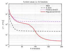
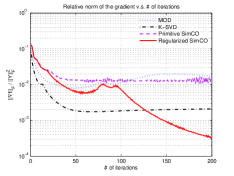
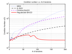
Figure 1: Starting with the same point, the convergence behaviors of MOD, K-SVD, primitive SimCO and regularized SimCO are different. In this particular example, only regularized SimCO avoids converging to a singular point.

The numerical results are presented in Figure 1. In the left sub-figure, we compare the learning performance in terms of $\left\|\bm{Y}-\bm{D}\bm{X}\right\|_{F}^{2}$. In the middle sub-figure, we study the behavior of the gradient $\nabla_{\bm{D}}f\left(\bm{D}\right)$ for different algorithms. In the right sub-figure, we depict the condition number of the dictionary defined as

$$\kappa\left(\bm{D}\right)=\underset{1\leq j\leq d}{\max}\;\lambda_{\max}\left(\bm{D}_{:,\Omega\left(:,j\right)}\right)/\lambda_{\min}\left(\bm{D}_{:,\Omega\left(:,j\right)}\right).$$

Here, note that $\kappa\left(\bm{D}_{{\rm true}}\right)=3.39$. The results in Figure 1 show that

1. When the number of iterations exceeds 50, MOD, K-SVD and primitive SimCO stop improving the training performance: the value of $f$ decreases very slowly with further iterations. Surprisingly, the gradients in these methods do not converge to zero. This implies that these methods do not converge to local minimizers. A more careful study reveals that these algorithms converge to points where the curvature (Hessian) of the objective function $f\left(\bm{D}\right)$ is large: the gradient of the objective function $\nabla_{\bm{D}}f$ changes dramatically in a small neighborhood.

2. The above phenomenon can be well explained by checking the ill-condition of the dictionary. After 100 iterations, the condition number $\kappa\left(\bm{D}\right)$ remains large ($>10$) for MOD, K-SVD, and primitive SimCO.

3. By adding a regularized term and choosing the regularization constant properly, regularized SimCO avoids the convergence to an ill-conditioned dictionary.

In fact, our simulations in Section VII-B show that the performance of primitive SimCO is not as good as other methods. We tracked all the simulated samples and found that it is because primitive SimCO may converge to a singular point very fast. Adding the regularization term significantly improves the performance (see Sections VII-B and VII-C). The necessity of regularized SimCO is therefore clear.

VII-B Experiments on Synthetic Data

The setting for synthetic data tests is summarized as follows. The training samples are generated via $\bm{Y}=\bm{D}_{{\rm true}}\bm{X}_{{\rm true}}$. Here, the columns of $\bm{D}_{{\rm true}}$ are randomly generated from the uniform distribution on the Stiefel manifold $\mathcal{U}_{m,1}$. Each column of $\bm{X}_{{\rm true}}$ contains exactly $S$ many non-zeros: the position of the non-zeros are uniformly distributed on the set ${\left[d\right]\choose S}=\left\{\left\{i_{1},\cdots,i_{S}\right\}:\;1\leq i_{k}\neq i_{\ell}\leq d\right\}$; and the values of the non-zeros are standard Gaussian distributed. In the tests, we fix $m=16$, $d=32$, and $S=4$, and change $n$, i.e., the number of training samples. Note that we intentionally choose $n$ to be small, which corresponds to the challenging case.

We first focus on the performance of dictionary update by assuming the true sparsity $\Omega_{{\rm true}}$ is available. Results are presented in Fig. 2. Note that the objective function of regularized SimCO is different from that of other methods. The ideal way to test regularized SimCO is to sequentially decrease the regularization constant $\mu$ to zero. In practice, we use the following simple strategy: the total number of iterations is set to 400; we change $\mu$ from $1e-1$ to $1e-2$, $1e-3$, and $1e-4$, for every 100 iterations. Simulations show that the average performance of regularized SimCO is consistently better than that of MOD and K-SVD. Note that there always exists a floor in reconstruction error that is proportional to noise. The normalized learning performance $\left\|\bm{Y}-\bm{D}\bm{X}\right\|_{F}^{2}/n$ is presented in Figure 2. The average performance of regularized SimCO is consistently better than that of MOD and K-SVD.

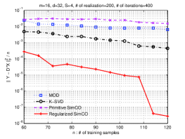
(a) Noiseless case.

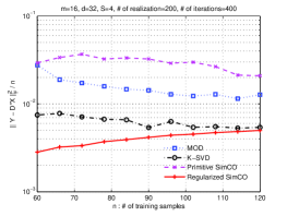
(b) Noisy case: SNR of training samples is 20dB. Note that there always exists a floor in reconstruction error that is proportional to noise.

Figure 2: Performance comparison of dictionary update (no sparse coding step).

Then we evaluate the overall dictionary learning performance by combining the dictionary update and sparse coding stages. For sparse coding, we adopt the OMP algorithm [25] as it has been intensively used for testing the K-SVD method in [10, 67]. The overall dictionary learning procedure is given in Algorithm 1. We refer to the iterations between sparse coding and dictionary learning stages as outer-iterations, and the iterations within the dictionary update stage as inner-iterations. In our test, the number of outer-iterations is set to 50, and the number of inner-iterations of is set to 1. Furthermore, in regularized SimCO, the regularized constant is set to $\mu=1e-1$ during the first 30 outer-iterations, and $\mu=0$ during the rest 20 outer-iterations. The normalized learning performance $\left\|\bm{Y}-\bm{D}\bm{X}\right\|_{F}^{2}/n$ is depicted in Figure 2. Again, the average performance of regularized SimCO is consistently better than that of other methods.

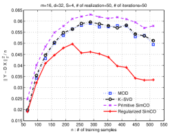
Figure 3: Performance comparison of dictionary learning using OMP for sparse coding.

Note that in the tests presented in this subsection, the performance of primitive SimCO is not as good as other methods. This motivates and justifies regularized SimCO.

VII-C Numerical Results for Image Denoising

As we mentioned in the introduction part, dictionary learning methods have many applications. In this subsection, we look at one particular application, i.e., image denoising. Here, a corrupted image with noise was used to train the dictionary: we take 1,000 (significantly less than 65,000 used in [67]) blocks (of size $8\times 8$) of the corrupted image as training samples. The number of codewords in the training dictionary is 256. For dictionary learning, we iterate the sparse coding and dictionary update stages for 10 times. The sparse coding stage is based on the OMP algorithm implemented in [67]. In the dictionary update stage, different algorithms are tested. For regularized SimCO, the regularization constant is set to $\mu=0.05$. During each dictionary update stage, the line search procedure is only performed once. After the whole process of dictionary learning, we use the learned dictionary to reconstruct the image. The reconstruction results are presented in Fig. 4. While all dictionary learning methods significantly improves the image SNRs, the largest gain was obtained from regularized SimCO.

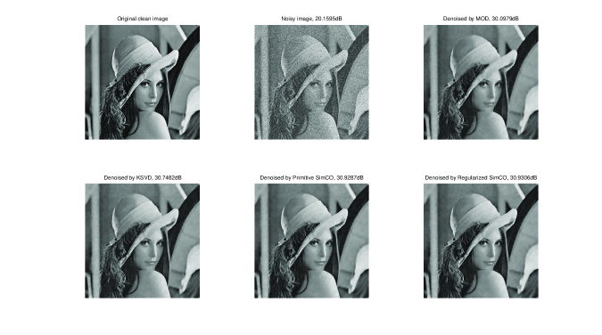
Figure 4: Example of the image denoising using dictionary learning. PSNR values in dB are given in sub-figure titles.

VII-D Comments on the Running Time

We compare the running time of different dictionary update algorithms in Table I. It is empirically observed that SimCO runs faster than K-SVD but slower than MOD. The speed-up compared with K-SVD comes from the simultaneous update of codewords. That SimCO is slower than MOD is not surprising for the following reasons: MOD also updates all the codewords simultaneously; and MOD only requires solving least-squares problems, which are much simpler than the optimization problem in SimCO.

Table I: Comparison of running time (in seconds) for dictionary learning. Note that sparse coding step is included in producing Fig. 3 and 4.

	MOD	K-SVD	Primitive SimCO	Regularized SimCO
Fig. 2(a)	$2.4\times 10^{4}$	$2.0\times 10^{5}$	$5.1\times 10^{4}$	$4.0\times 10^{4}$
Fig. 2(b)	$2.3\times 10^{4}$	$1.9\times 10^{5}$	$5.0\times 10^{4}$	$4.0\times 10^{4}$
Fig. 3	$1.5\times 10^{4}$	$3.7\times 10^{4}$	$3.1\times 10^{4}$	$3.1\times 10^{4}$
Fig. 4	1.42	29.43	2.63	2.72

VIII Conclusions

We have presented a new framework for dictionary update. It is based on optimization on manifolds and allows a simultaneous update of all codewords and the corresponding coefficients. Two algorithms, primitive and regularized SimCO have been developed. On the theoretical aspect, we have established the equivalence between primitive SimCO and K-SVD when only one codeword update is considered. On the more practical side, numerical results are presented to show the good learning performance and fast running speed of regularized SimCO.

-A Proof of Theorem 1

The following notations are repeatedly used in the proofs. Consider the singular value decomposition $\bm{A}=\sum_{i=1}^{m}\lambda_{i}\bm{u}_{\bm{A},i}\bm{v}_{\bm{A},i}^{T}$, where $\lambda_{1}>\lambda_{2}\geq\cdots\geq\lambda_{m}\geq 0$ are the singular values, and $\bm{u}_{\bm{A},i}$ and $\bm{v}_{\bm{A},i}$ are the left and right singular vectors corresponding to $\lambda_{i}$ respectively. It is clear that the objective function $f\left(\bm{u}\right)=\inf_{\bm{w}\in\mathbb{R}^{n}}\;\left\|\bm{A}-\bm{u}\bm{w}^{T}\right\|_{F}^{2}$ has two global minimizers $\pm\bm{u}_{\bm{A},1}$. For a given $\bm{u}\in\mathcal{U}_{m,1}$, the angle between $\bm{u}$ and the closest global minimizer is defined as

$$\theta=\mbox{cos}^{-1}\left|\left\langle\bm{u},\bm{u}_{\bm{A},1}\right\rangle\right|.$$

The crux of the proof is that along the gradient descent path, the angle $\theta$ is monotonically decreasing. Suppose that the starting angle is less than $\pi/2$. Then the only stationary points are when the angle $\theta$ is zero. Hence, the gradient descent search converges to a global minimizer. The probability one part comes from that the starting angle equals to $\pi/2$ with probability zero.

To formalize the idea, it is assumed that the starting point $\bm{u}_{0}\in\mathcal{U}_{m,1}$ is randomly generated from the uniform distribution on the Stiefel manifold. Define a set $\mathcal{B}\subset\mathcal{U}_{m,1}$ to describe the set of “bad” starting points. It is defined by

$$\mathcal{B}=\left\{\bm{u}\in\mathcal{U}_{m,1}:\;\bm{u}^{T}\bm{u}_{\bm{A},1}=0\right\},$$

which contains all unit vectors that are orthogonal to $\bm{u}_{\bm{A},1}$. According to [68], under the uniform measure on $\mathcal{U}_{m,1}$, the measure of the set $\mathcal{B}$ is zero. As a result, the starting point $\bm{u}_{0}\notin\mathcal{B}$ with probability one. The reason that we refer to $\mathcal{B}$ as the set of “bad” starting points is explained by the following lemma.

Lemma 4.

Starting from any $\bm{u}_{0}\in\mathcal{B}$, a gradient descent path stays in the set $\mathcal{B}$.

Proof:

This lemma can be proved by computing the gradient of $f$ at a $\bm{u}\in\mathcal{B}$. Let $\bm{w}_{\bm{u}}\in\mathbb{R}^{n}$ be the optimal solution of the least squares problem in $f\left(\bm{u}\right)=\inf_{\bm{w}\in\mathbb{R}^{n}}\;\left\|\bm{A}-\bm{u}\bm{w}^{T}\right\|_{F}^{2}$. It can be verified that $\bm{w}_{\bm{u}}=\bm{A}^{T}\bm{u}$ and $\nabla f=-2\left(\bm{A}-\bm{u}\bm{w}_{\bm{u}}^{T}\right)\bm{w}_{\bm{u}}$. It is clear that

$$\nabla f =-2\left(\bm{A}-\bm{u}\bm{w}_{\bm{u}}^{T}\right)\bm{w}_{\bm{u}}=-2\left(\bm{A}-\bm{u}\bm{u}^{T}\bm{A}\right)\bm{A}^{T}\bm{u}$$

$$=-2\sum_{i}\lambda_{i}^{2}\bm{u}_{\bm{A},i}\bm{u}_{\bm{A},i}^{T}\bm{u}+2\bm{u}\left(\bm{u}^{T}\bm{A}\bm{A}^{T}\bm{u}\right)$$

When $\bm{u}_{0}\in\mathcal{B}$, it holds that $\left\langle\bm{u}_{0},\bm{u}_{\bm{A},1}\right\rangle=0$ and $\left\langle\nabla f\left(\bm{u}_{0}\right),\bm{u}_{\bm{A},1}\right\rangle=0$. Since both $\bm{u}_{0}$ and the gradient descent direction are orthogonal to $\bm{u}_{\bm{A},1}$, the gradient descent path starting from $\bm{u}_{0}\in\mathcal{B}$ stays in $\mathcal{B}$. ∎

Now consider a starting points $\bm{u}_{0}\notin\mathcal{B}$. We shall show that the angle $\theta$ is monotonically decreasing along the gradient descent path. Towards this end, the notions of directional derivative play an important role. View $\theta$ as a function of $\bm{u}\in\mathcal{U}_{m,1}$. The directional derivative of $\theta$ at $\bm{u}\in\mathcal{U}_{m,1}$ along a direction vector $\bm{h}\in\mathbb{R}^{m}$, denoted by $\nabla_{\bm{h}}\theta\in\mathbb{R}$, is defined as

$$\nabla_{\bm{h}}\theta=\underset{\epsilon\rightarrow 0}{\lim}\frac{\theta\left(\bm{u}+\epsilon\bm{h}\right)-\theta\left(\bm{u}\right)}{\epsilon}.$$

Note the relationship between directional derivative and gradient given by $\nabla_{\bm{h}}\theta=\left\langle\nabla\theta,\bm{h}\right\rangle$. With this definition, the following lemma plays the central role in establishing Theorem 1.

Lemma 5.

Consider a $\bm{u}\in\mathcal{U}_{m,1}$ such that $\theta\left(\bm{u}\right):=\cos^{-1}\left(\left|\left\langle\bm{u},\bm{u}_{\bm{A},1}\right\rangle\right|\right)\in\left(0,\pi/2\right)$. Let $\bm{h}_{f}=-\nabla f\left(\bm{u}\right)$ be the gradient of the objective function $f$ at $\bm{u}$. Then it holds $\nabla_{\bm{h}_{f}}\theta<0$.

The proof of this lemma is detailed in Appendix -B.

The implications of this lemma are twofold. First, it implies that $\bm{h}_{f}=-\nabla f\neq\bm{0}$ for all $\bm{u}$ such that $\theta\left(\bm{u}\right)\in\left(0,\pi/2\right)$. Hence, the only possible stationary points in $\mathcal{U}_{m,1}\backslash\mathcal{B}$ are $\bm{u}_{\bm{A},1}$ and $-\bm{u}_{\bm{A},1}$. Second, starting from $\bm{u}_{0}\in\mathcal{B}$, the angle $\theta$ decreases along the gradient descent path. As a result, a gradient descent path will not enter $\mathcal{B}$. It will converge to $\bm{u}_{\bm{A},1}$ or $-\bm{u}_{\bm{A},1}$. Theorem 1 is therefore proved.

-B Proof of Lemma 5

This appendix is devoted to prove Lemma 5, i.e., $\nabla_{\bm{h}_{f}}\theta<0$. Note that $\nabla_{\bm{h}_{f}}\theta=\left\langle\bm{h}_{f},\nabla\theta\right\rangle=\left\langle-\nabla f,\nabla\theta\right\rangle=\nabla_{-\nabla\theta}f$. It suffices to show that $\nabla_{-\nabla\theta}f<0$.

Towards this end, the following definitions are useful. Define $s=\mbox{sign}\left(\bm{u}^{T}\bm{u}_{\bm{A},1}\right)$. Then the vector $s\bm{u}_{\bm{A},1}$ is one of the two global minimizers that is the closest to $\bm{u}$. It can be also verified that $\theta=\cos^{-1}\left\langle\bm{u},s\bm{u}_{\bm{A},1}\right\rangle$. Furthermore, suppose that $\theta\in\left(0,\pi/2\right)$. Define

$$\bm{h}_{\theta}=\frac{s\bm{u}_{\bm{A},1}-\bm{u}\cos\theta}{\sin\theta},\;{\rm and}\;\bm{u}_{\perp}=\frac{\bm{u}-s\bm{u}_{\bm{A},1}\cos\theta}{\sin\theta}.$$

Clearly, vectors $\bm{h}_{\theta}$ and $\bm{u}_{\perp}$ are well-defined when $\theta\in\left(0,\pi/2\right)$. The relationship among $\bm{u}$, $\bm{u}_{\bm{A},1}$, $\bm{h}_{\theta}$ and $\bm{u}_{\perp}$ is illustrated in Figure 5. Intuitively, the vector $\bm{h}_{\theta}$ is the tangent vector that pushes $\bm{u}$ towards the global minimizer $s\bm{u}_{\bm{A},1}$.

Figure 5: Illustration of $\bm{u}$, $\bm{u}_{\bm{A},1}$, $\bm{h}_{\theta}$ and $\bm{u}_{\perp}$.

In the following, we show that $\nabla_{-\nabla\theta}f=\nabla_{\bm{h}_{\theta}}f$ if we restrict $\bm{u}\in\mathcal{U}_{m,1}$. By the definition of the directional derivative, one has

$$\nabla_{-\nabla\theta}\bm{u} =\underset{\epsilon\rightarrow 0}{\lim}\frac{\bm{u}-\epsilon\nabla\theta}{\left\|\bm{u}-\epsilon\nabla\theta\right\|}.$$

Note that

$$\nabla\theta =\nabla\left(\cos^{-1}\left(\cos\theta\right)\right)$$

$$=-\frac{1}{\sqrt{1-\cos^{2}\theta}}\nabla\left\langle\bm{u},s\bm{u}_{\bm{A},1}\right\rangle=-\frac{1}{\sin\theta}\left(s\bm{u}_{\bm{A},1}\right).$$

Since $s\bm{u}_{\bm{A},1}=\bm{u}\cos\theta+\bm{h}_{\theta}\sin\theta$, one has

$$\bm{u}-\epsilon\nabla\theta =\bm{u}+\frac{\epsilon}{\sin\theta}\left(s\bm{u}_{\bm{A},1}\right)$$

$$=\bm{u}\left(1+\epsilon\cos\theta/\sin\theta\right)+\epsilon\bm{h}_{\theta}.$$

Substitute it back to $\nabla_{-\nabla\theta}\bm{u}$. One has $\nabla_{-\nabla\theta}\bm{u}=\bm{h}_{\theta}.$ In other words, if $\bm{u}\in\mathcal{U}_{m,1}$, then $\nabla_{-\nabla\theta}f=\nabla_{\bm{h}_{\theta}}f.$

To compute $\nabla_{\bm{h}_{\theta}}f$, note that $f\left(\bm{u}\right)=\left\|\bm{A}-\bm{u}\bm{w}_{\bm{u}}^{T}\right\|_{F}^{2}=\left\|\bm{A}\right\|_{F}^{2}-\left\|\bm{u}^{T}\bm{A}\right\|_{2}^{2}.$ Now define

$$g\left(\bm{u}\right)=\left\|\bm{u}^{T}\bm{A}\right\|_{2}^{2}.$$

Then clearly $\nabla_{\bm{h}_{\theta}}f=-\nabla_{\bm{h}_{\theta}}g$. To proceed, we also decompose $\bm{A}$ as follows. Recall the SVD of $\bm{A}$ given by $\bm{A}=\sum_{i=1}^{m}\lambda_{i}\bm{u}_{\bm{A},i}\bm{v}_{\bm{A},i}^{T}$. Let $\bm{U}_{\bm{A},\perp}\in\mathcal{U}_{m,m-1}$ contain the left singular vectors corresponding to $\lambda_{2},\cdots,\lambda_{m}$, i.e., $\bm{U}_{\bm{A},\perp}=\left[\bm{u}_{\bm{A},2},\cdots,\bm{u}_{\bm{A},m}\right]$. Similarly define $\bm{V}_{\bm{A},\perp}$. Then,

$$\bm{A} =\left[\bm{u}_{\bm{A},1},\bm{U}_{\bm{A},\perp}\right]\mbox{diag}\left(\left[\lambda_{1},\cdots,\lambda_{m}\right]\right)\left[\begin{array}[]{c}\bm{v}_{\bm{A},1}^{T}\\ \bm{V}_{\bm{A},\perp}^{T}\end{array}\right]$$

$$=\left[\bm{u}_{\bm{A},1},\bm{U}_{\bm{A},\perp}\right]\left[\bm{w}_{\bm{A},1},\bm{W}_{\bm{A},\perp}\right]^{T},$$

where $\bm{w}_{\bm{A},i}=\lambda_{i}\bm{v}_{\bm{A},i}$ for $i=1,\cdots,m$, and $\bm{W}_{\bm{A},\perp}=\left[\bm{w}_{\bm{A},2},\cdots,\bm{w}_{\bm{A},m}\right]$. It is straightforward to verify that $\bm{w}_{\bm{A}}^{T}\bm{W}_{\bm{A},\perp}=\bm{0}$.

The function $g\left(\bm{u}\right)$ can be decomposed into two parts. Note that

$$g\left(\bm{u}\right) =\left\|\bm{u}^{T}\left[\bm{u}_{\bm{A},1},\bm{U}_{\bm{A},\perp}\right]\left[\bm{w}_{\bm{A},1},\bm{W}_{\bm{A},\perp}\right]^{T}\right\|_{2}^{2}$$

$$=\left\|\bm{u}^{T}\bm{u}_{\bm{A},1}\bm{w}_{\bm{A},1}^{T}\right\|_{2}^{2}+\left\|\bm{u}^{T}\bm{U}_{\bm{A},\perp}\bm{W}_{\bm{A},\perp}^{T}\right\|_{2}^{2}$$

$$\quad+2\left\langle\bm{u}^{T}\bm{u}_{\bm{A},1}\bm{w}_{\bm{A},1}^{T},\bm{u}^{T}\bm{U}_{\bm{A},\perp}\bm{W}_{\bm{A},\perp}^{T}\right\rangle$$

$$=\left\|\bm{u}^{T}\bm{u}_{\bm{A},1}\bm{w}_{\bm{A},1}^{T}\right\|_{2}^{2}+\left\|\bm{u}^{T}\bm{U}_{\bm{A},\perp}\bm{W}_{\bm{A},\perp}^{T}\right\|_{2}^{2},$$

where the last equality follows from that $\bm{W}_{\bm{A},\perp}^{T}\bm{w}_{\bm{A}}=\bm{0}$ and hence

$$\left\langle\bm{u}^{T}\bm{u}_{\bm{A},1}\bm{w}_{\bm{A},1}^{T},\bm{u}^{T}\bm{U}_{\bm{A},\perp}\bm{W}_{\bm{A},\perp}^{T}\right\rangle=0.$$

To further simplify $g\left(\bm{u}\right)$, note that $\cos\theta=\left|\bm{u}^{T}\bm{u}_{\bm{A}}\right|$. Furthermore, it is straightforward to verify that the projection of $\bm{u}$ on $\mbox{span}\left(\bm{U}_{\bm{A},\perp}\right)$ is given by $\bm{U}_{\bm{A},\perp}\bm{U}_{\bm{A},\perp}^{T}\bm{u}=\bm{u}_{\perp}\sin\theta$. Define $\bm{u}_{R}=\bm{U}_{\bm{A},\perp}^{T}\bm{u}_{\perp}\in\mathbb{R}^{m-1}$. Then, $\left\|\bm{u}_{R}\right\|=1$ and

$$\left\|\bm{u}^{T}\bm{U}_{\bm{A},\perp}\bm{W}_{\bm{A},\perp}^{T}\right\|_{2}^{2}$$

$$=\sin^{2}\theta\left\|\bm{u}_{\perp}^{T}\bm{U}_{\bm{A},\perp}\bm{W}_{\bm{A},\perp}^{T}\right\|_{2}^{2}$$

$$=\sin^{2}\theta\bm{u}_{R}^{T}\mbox{diag}\left(\left[\lambda_{2}^{2},\cdots,\lambda_{m}^{2}\right]\right)\bm{u}_{R}^{T}.$$

Hence,

$$g\left(\bm{u}\right)=\cos^{2}\theta\cdot\lambda_{1}+\sin^{2}\theta\bm{u}_{R}^{T}\mbox{diag}\left(\left[\lambda_{2}^{2},\cdots,\lambda_{m}^{2}\right]\right)\bm{u}_{R}.$$

It is now ready to decide the sign of $\nabla_{\bm{h}_{\theta}}g$. It is straightforward to verify that

$$\nabla_{\bm{h}_{\theta}}\cos\theta=\underset{\epsilon\rightarrow 0}{\lim}\left\langle\frac{\bm{u}+\epsilon\bm{h}_{\theta}}{\sqrt{1+\epsilon^{2}}},s\bm{u}_{\bm{A},1}\right\rangle=\sin\theta,$$

and similarly $\nabla_{\bm{h}_{\theta}}\sin\theta=-\cos\theta.$ Therefore,

$$\nabla_{\bm{h}_{\theta}}\bm{u}_{\perp} =\nabla_{\bm{h}_{\theta}}\left(\frac{\bm{u}--\cos\theta s\bm{u}_{\bm{A},1}}{\sin\theta}\right)$$

$$=\frac{\bm{h}_{\theta}\sin\theta+\bm{u}\cos\theta-s\bm{u}_{\bm{A},1}}{\sin^{2}\theta}$$

$$=\frac{s\bm{u}_{\bm{A},1}-s\bm{u}_{\bm{A},1}}{\sin^{2}\theta}=\bm{0},$$

and $\nabla_{\bm{h}_{\theta}}\bm{u}_{R}=\nabla_{\bm{h}_{\theta}}\left(\bm{U}_{\bm{A},\perp}^{T}\bm{u}_{\perp}\right)=\bm{0}$. Hence, one has

$$\nabla_{\bm{h}_{\theta}}g =\sin 2\theta\left(\lambda_{1}-\bm{u}_{R}^{T}\mbox{diag}\left(\left[\lambda_{2}^{2},\cdots,\lambda_{m}^{2}\right]\right)\bm{u}_{R}\right).$$

Note that

$$\bm{u}_{R}^{T}\mbox{diag}\left(\left[\lambda_{2}^{2},\cdots,\lambda_{m}^{2}\right]\right)\bm{u}_{R}$$

$$\leq\bm{u}_{R}^{T}\mbox{diag}\left(\left[\lambda_{2}^{2},\cdots,\lambda_{2}^{2}\right]\right)\bm{u}_{R}=\lambda_{2}<\lambda_{1}.$$

It can be concluded that when $\theta\in\left(0,\pi/2\right)$, $\nabla_{\bm{h}_{\theta}}g>0$ and $\nabla_{\bm{h}_{\theta}}f=-\nabla_{\bm{h}_{\theta}}g<0$. Lemma 5 is therefore proved.

References

- [1] P. Foldiak, “Forming sparse representations by local anti-Hebbian learning,” Biolog. Cybern., vol. 64, pp. 165–170, 1990.
- [2] M. S. Lewicki and T. J. Sejnowski, “Learning overcomplete representations,” Neural Comput., vol. 12, no. 2, pp. 337–365, 2000.
- [3] J. Tropp, “Topics in sparse approximations,” Ph.D. dissertation, University of Texas at Austin, 2004.
- [4] B. A. Olshausen, C. F. Cadieu, and D. K. Warland, “Learning real and complex overcomplete representations from the statistics of natural images,” Proc. SPIE, vol. 7446, 2009.
- [5] B. A. Olshausen and D. J. Field, “Emergence of simple-cell receptive field properties by learning a sparse code for natural images,” Nature, vol. 381, pp. 607–609, 1996.
- [6] I. Tošić and P. Frossard, “Dictionary learning for stereo image representation,” IEEE Trans. Image Process., vol. 20, no. 4, pp. 921–934, 2011.
- [7] M. Zibulevsky and B. A. Pearlmutter, “Blind source separation by sparse decomposition of a signal dictionary,” Neural Comput., vol. 13, no. 4, pp. 863–882, 2001.
- [8] R. Gribonval, “Sparse decomposition of stereo signals with matching pursuit and application to blind separation of more than two sources from a stereo mixture,” in IEEE Int. Conf. Acoust., Speech Signal Process., vol. 3, 2002, pp. 3057–3060.
- [9] T. Xu and W. Wang, “Methods for learning adaptive dictionary in underdetermined speech separation,” in IEEE Int. Conf. Machine Learning for Signal Processing., Beijing, China, 2011.
- [10] M. Aharon, M. Elad, and A. Bruckstein, “K-SVD: An algorithm for designing overcomplete dictionaries for sparse representation,” IEEE Trans. Signal Process., vol. 54, no. 11, pp. 4311–4322, 2006.
- [11] M. G. Jafari and M. D. Plumbley, “Fast dictionary learning for sparse representations of speech signals,” IEEE J. Selected Topics in Signal Process., vol. 5, no. 5, pp. 1025–1031, 2011.
- [12] P. Schmid-Saugeon and A. Zakhor, “Dictionary design for matching pursuit and application to motion-compensated video coding,” IEEE Trans. Circuits Syst. Video Technol., vol. 14, no. 6, pp. 880–886, 2004.
- [13] E. Kokiopoulou and P. Frossard, “Semantic coding by supervised dimensionality reduction,” IEEE Trans. Multimedia, vol. 10, no. 5, pp. 806–818, 2008.
- [14] M. D. Plumbley, T. Blumensath, L. Daudet, R. Gribonval, and M. E. Davies, “Sparse representations in audio and music: From coding to source separation,” Proceedings of IEEE, vol. 98, no. 6, pp. 995–1005, 2010.
- [15] K. Huang and S. Aviyente, “Sparse representation for signal classification,” in Conf. Neural Information Processing Systems, 2007.
- [16] J. Mairal, F. Bach, J. Ponce, G. Sapiro, and A. Zisserman, “Discriminative learned dictionaries for local image analysis,” in IEEE Int. Conf. Computer Vision and Pattern Recognition, 2008, pp. 1–8.
- [17] K. Schnass and P. Vandergheynst, “A union of incoherent spaces model for classification,” in IEEE Int. Conf. Acoustics, Speech, and Signal Processing, 2010, pp. 5490–5493.
- [18] J. Wright, A. Yang, A. Ganesh, S. Sastry, and Y. Ma, “Robust face recognition via sparse representation,” IEEE Trans. Pattern Anal. Mach. Intell., vol. 31, no. 2, pp. 210–227, 2009.
- [19] V. Cevher and A. Krause, “Greedy dictionary selection for sparse representation,” in Proc. NIPS Workshop on Discrete Optimization in Machine Learning, Vancouver, Canada, December 2009.
- [20] A. Adler, V. Emiya, M. G. Jafari, M. Elad, R. Gribonval, and M. D. Plumbley, “Audio inpainting,” IEEE Trans. on Audio, Speech and Language Processing, submitted, 2011. [Online]. Available: http://www.cs.technion.ac.il/ elad/publications/journals
- [21] R. G. Baraniuk, E. J. Candès, M. Elad, and Y. Ma, “Applications of sparse representation and compressive sensing,” Proceedings of the IEEE, vol. 98, no. 6, pp. 906–909, 2010.
- [22] S. Chen, D. Donoho, and M. Saunders, “Atomic decomposition by basis pursuit,” SIAM J. Sci. Comput., vol. 20, no. 1, pp. 33–61, 1999.
- [23] S. G. Mallat and Z. Zhang, “Matching pursuits with time-frequency dictionaries,” IEEE Trans. Signal Process., vol. 41, no. 12, pp. 3397–3415, 1993.
- [24] Y. C. Pati, R. Rezaiifar, and P. S. Krishnaprasad, “Orthogonal matching pursuit: recursive function approximation with applications to wavelet decomposition,” in IEEE Asilomar Conference on Signals, Systems and Computers, 1993, pp. 40–44.
- [25] J. Tropp and A. C. Gilbert, “Signal recovery from random measurements via orthogonal matching pursuit,” IEEE Trans. Inf. Theory, vol. 53, no. 12, pp. 4655–4666, 2007.
- [26] W. Dai and O. Milenkovic, “Subspace pursuit for compressive sensing signal reconstruction,” IEEE Trans. Inform. Theory, vol. 55, pp. 2230–2249, 2009.
- [27] D. Needell and J. A. Tropp, “CoSaMP: Iterative signal recovery from incomplete and inaccurate samples,” Appl. Comp. Harmonic Anal., vol. 26, no. 3, pp. 301–321, May 2009.
- [28] R. Tibshirani, “Regression shrinkage and selection via the lasso,” J. R. Stat. Soc. Ser. B (Method.), vol. 58, no. 1, pp. 267–288, 1996.
- [29] I. Gorodnitsky and B. Rao, “Sparse signal reconstruction from limited data using FOCUSS: a re-weighted minimum norm algorithm,” IEEE Trans. Signal Process., vol. 45, no. 3, pp. 600–616, 1997.
- [30] T. Blumensath and M. E. Davies, “Gradient pursuits,” IEEE Trans. Signal Process., vol. 56, no. 6, pp. 2370–2382, 2008.
- [31] I. W. Selesnick, R. G. Baraniuk, and N. C. Kingsbury, “The dual-tree complex wavelet transform,” IEEE Signal Process Mag., vol. 22, no. 6, pp. 123–151, 2005.
- [32] E. J. Candès and D. L. Donoho, “Curvelets - a surprisingly effective nonadaptive representation for objects with edges,” Curves and Surfaces, 2999.
- [33] M. N. Do and M. Vetterli, “The contourlet transform: An efficient directional multiresolution image representation,” IEEE Trans. Image Process., vol. 14, no. 12, pp. 2091–2106, 2005.
- [34] E. LePennec and S. Mallat, “Sparse geometric image representations with bandelets,” IEEE Trans. Image Process., vol. 14, no. 4, pp. 423–438, 2005.
- [35] B. A. Olshausen and D. J. Field, “Sparse coding with an overcomplete basis set: A strategy employed by V1,” Vis. Res., vol. 37, no. 23, pp. 3311–3325, 1997.
- [36] K. Engan, S. Aase, and J. H. Husøy, “Method of optimal directions for frame design,” in IEEE Int. Conf. Acoustics, Speech, and Signal Processing, vol. 5, 1999, pp. 2443–2446.
- [37] K. Kreutz-Delgado, J. Murray, B. Rao, K. Engan, T.-W. Lee, and T. J. Sejnowski, “Dictionary learning algorithms for sparse representation,” Neural Comput., vol. 15, no. 2, pp. 349–396, 2003.
- [38] D. P. Wipf and B. D. Rao, “Sparse bayesian learning for basis selection,” IEEE Trans. Signal Process., vol. 52, no. 8, pp. 2153–2164, 2004.
- [39] M. D. Plumbley, “Dictionary learning for L1-exact sparse coding,” Lect. Notes Comput. Sci., vol. 4666, pp. 406–413, 2007.
- [40] M. G. Jafari and M. D. Plumbley, “Speech denoising based on a greedy adaptive dictionary algorithm,” in European Signal Processing Conf., 2009, pp. 1423–1426.
- [41] R. Gribonval and K. Schnass, “Dictionary identification - sparse matrix factorisation via l1 minimisation,” IEEE Trans. Inf. Theory, vol. 56, no. 7, pp. 3523–3539, 2010.
- [42] Q. Geng, H. Wang, and J. Wright, “On the local correctness of L-1 minimization for dictionary learning,” arXiv:1101.5672, 2011.
- [43] R. Rubinstein, A. M. Bruckstein, and M. Elad, “Dictionaries for sparse representation modelling,” Proceedings of IEEE, vol. 98, no. 6, pp. 1045–1057, 2010.
- [44] K. Engan, K. Skretting, and J. H. Husøy, “Family of iterative LS-based dictionary learning algorithms, ILS-DLA, for sparse signal representation,” Dig. Signal Process., vol. 17, no. 1, pp. 32–49, 2007.
- [45] K. Skretting and K. Engan, “Recursive least squares dictionary learning algorithm,” IEEE Trans. Signal Process., vol. 58, no. 4, pp. 2121–2130, 2010.
- [46] M. Yaghoobi, T. Blumensath, and M. E. Davies, “Dictionary learning for sparse approximations with the majorization method,” IEEE Trans. Signal Process., vol. 57, no. 6, pp. 2178–2191, 2009.
- [47] M. Yaghoobi, L. Daudet, and M. E. Davies, “Parametric dictionary design for sparse coding,” IEEE Trans. Signal Process., vol. 57, no. 12, pp. 4800–4810, 2009.
- [48] P. Sallee and B. A. Olshausen, “Learning sparse multiscale image representations,” in Conf. Neural Information Processing Systems, 2003.
- [49] C. Cadieu and B. A. Olshausen, “Learning transformational invariants from time-varying natural images,” in Proc. Conf. Neural Information Processing Systems, 2088.
- [50] T. Blumensath and M. Davies, “Sparse and shift-invariant representations of music,” IEEE Trans. Speech Audio Process., vol. 14, no. 1, pp. 50–57, 2006.
- [51] B. Mailhé, S. Lesage, R. Gribonval, F. Bimbot, and P. Vandergheynst, “Shift invariant dictionary learning for sparse representations: Extending K-SVD,” in European Signal Processing Conf., vol. 4, 2008.
- [52] M. Aharon and M. Elad, “Sparse and redundant modeling of image content using an image-signature-dictionary,” SIAM J. Imaging Sci., vol. 1, no. 3, pp. 228–247, 2008.
- [53] P. Smaragdis, B. Raj, and M. Shashanka, “Sparse and shift-invariant feature extraction from non-negative data,” in IEEE Int. Conf. on Audio and Speech Signal Processing, 2008, pp. 2069–2072.
- [54] R. Gribonval and M. Nielsen, “Sparse representations in unions of bases,” IEEE Trans. Inf. Theory, vol. 49, no. 12, pp. 3320–3325, 2003.
- [55] P. Jost, P. Vandergheynst, S. Lesage, and R. Gribonval, “BMoTIF: An efficient algorithm for learning translation invariant dictionaries,” in IEEE Int. Conf. Acoust., Speech, Signal Process., vol. 5, 2006, pp. 857–860.
- [56] K. Labusch, E. Barth, and T. Martinetz, “Robust and fast learning of sparse codes with stochastic gradient descent,” IEEE J. Selected Topics in Signal Process., vol. 5, no. 5, pp. 1048–1060, 2011.
- [57] J. Mairal, F. Bach, J. Ponce, and G. Sapiro, “Online learning for matrix factorization and sparse coding,” J. Mach. Learn. Res., vol. 11, pp. 16–60, 2010.
- [58] G. Monaci, P. Vandergheynst, and F. T. Sommer, “Learning bimodal structure in audio-visual data,” IEEE Trans. Neural Netw., vol. 20, no. 12, pp. 1898–1910, 2009.
- [59] A. L. Casanovas, G. Monaci, P. Vandergheynst, and R. Gribonval, “Blind audiovisual source separation based on sparse redundant representations,” IEEE Trans. Multimedia, vol. 12, no. 5, pp. 358–371, 2010.
- [60] I. Tošić and P. Frossard, “Dictionary learning: what is the right representation for my signal,” IEEE Signal Process. Mag., vol. 28, no. 2, pp. 27–38, March 2011.
- [61] E. Candes and T. Tao, “Decoding by linear programming,” vol. 51, no. 12, pp. 4203–4215, Dec. 2005.
- [62] A. Edelman, T. A. Arias, and S. T. Smith, “The geometry of algorithms with orthogonality constraints,” SIAM J. Matrix Anal. Appl., vol. 20, no. 2, pp. 303–353, 1999.
- [63] W. Dai, E. Kerman, and O. Milenkovic, “A geometric approach to low-rank matrix completion,” IEEE Trans. Inform. Theory, 2011, accepted. [Online]. Available: http://arxiv.org/abs/1006.2086
- [64] P.-A. Absil, R. Mahony, and R. Sepulchre, Optimization Algorithms on Matrix Manifolds. Princeton University Press, 2008.
- [65] J. Nocedal and S. J. Wright, Numerical Optimization. Springer, 2006.
- [66] W. H. Press, S. A. Teukolsky, W. T. Vetterling, and B. P. Flannery, Numerical Recipes: The Art of Scientific Computing, 3rd ed. Cambridge University Press, 2007, ch. 10.2. Golden Section Search in One Dimension.
- [67] M. Elad and M. Aharon, “Image denoising via sparse and redundant representations over learned dictionaries,” IEEE Transactions on Image Processing, vol. 15, no. 12, pp. 3736 –3745, dec. 2006.
- [68] W. Dai, Y. Liu, and B. Rider, “Quantization bounds on Grassmann manifolds and applications to MIMO systems,” IEEE Trans. Inform. Theory, vol. 54, no. 3, pp. 1108–1123, March 2008.