Asymptotic enumeration of Minimal Automata

Abstract.

We determine the asymptotic proportion of minimal automata, within $n$-state accessible deterministic complete automata over a $k$-letter alphabet, with the uniform distribution over the possible transition structures, and a binomial distribution over terminal states, with arbitrary parameter $b$. It turns out that a fraction $\sim 1-C(k,b)\,n^{-k+2}$ of automata is minimal, with $C(k,b)$ a function, explicitly determined, involving the solution of a transcendental equation.

1. Introduction

To any regular language, one can associate in a unique way its minimal automaton, i.e. the only accessible complete deterministic automaton recognizing the language, with minimal number of states. Therefore the space complexity of a regular language can be seen as the number of states of its minimal automaton. The worst-case complexity of algorithms dealing with finite automata is most of times known [29]. But the average-case analysis of algorithms requires weighted sums on the set of possible realizations, and in particular the enumeration of the objects that are handled [10]. Therefore a precise enumeration is often required for the algorithmic study of regular languages.

The enumeration of finite automata according to various criteria (with or without initial state [19], non-isomorphic [14], up to permutation of the labels of the edges [14], with a strongly connected underlying graph [22, 19, 27, 20], acyclic [23],…) has been investigated since the fifties.

In [19] Korshunov determines the asymptotic estimate of the number of accessible complete and deterministic $n$-state automata over a finite alphabet. His derivation, and even the formulation of the result, are quite complicated. In [4] a reformulation of Korshunov’s result leads to an estimate of the number of such automata involving the Stirling number of the second kind. On the other side, in [21] a different simplification of the involved expressions is achieved, by highlighting the role of the Lagrange Inversion Formula in the analysis.

A natural question is to ask which is the fraction of minimal automata, among accessible complete and deterministic automata of a given size $n$ and alphabet cardinality $k$. Nicaud [26] shows that, asymptotically, half of the complete deterministic accessible automata over a unary alphabet are minimal, thus solving the question for $k=1$. Using REGAL, a C++-library for the random generation of automata, the proportion of minimal automata amongst complete deterministic accessible ones experimentally seems to be $85,32\%$ for a $2$-letter alphabet and more than $99,99\%$. for a larger alphabet [2].

In this paper we solve this question for a generic integer $k\geq 2$. At a slightly higher level of generality, we give a precise estimation of the asymptotic proportion of minimal automata, within $n$-state accessible deterministic complete automata over a $k$-letter alphabet, for the uniform distribution over the possible transition structures, and a binomial distribution over terminal states, with arbitrary parameter $0<b<1$ (the uniform case corresponding to $b=\frac{1}{2}$). Our theoretical results are in agreement with the experimental ones.

The paper is organized as follows. In Section 2 we recall some basic notions of automata theory, and we set a list a notations that will be used in the remainder of the paper. Then, we state our main theorem, and give a short and simple heuristic argument. In Section 3 we give a detailed description of the proof structure, and its subdivision into separate lemmas. In Section 4 we prove in detail the most difficult lemmas, and give indications for those that are provable through standard methods. Finally, in Section 5 we discuss some of the implications of our result.

2. Statement of the result

For a given set $E$, $|E|$ denotes the cardinal of $E$. The symbol $[n]$ denotes the canonical $n$-element set $\{1,2,\ldots,n\}$. Let $\mathcal{E}$ be a Boolean condition, the Iverson bracket $[\negthinspace[{\mathcal{E}}]\negthinspace]$ is equal to $1$ if $\mathcal{E}=\textrm{true}$ and $0$ otherwise. We use $\mathbb{E}{(}X)$ to denote the expectation of the quantifier $X$, and $\mathbb{P}{(}\mathcal{E})=\mathbb{E}{(}[\negthinspace[{\mathcal{E}}]\negthinspace])$ for the probability of the event $\mathcal{E}$. For $\{\mathcal{E}_{i}\}$ a collection of events, we define a shortcut for the first moment

$${\bm{m}}(\{\mathcal{E}_{i}\}):=\sum_{i}\,\mathbb{P}{(}\mathcal{E}_{i})=\mathbb{E}{}\Big{(}\sum_{i}\;[\negthinspace[{\mathcal{E}_{i}}]\negthinspace]\Big{)}\,.$$ (1)

If $p(c)$ is the probability that exactly $c$ events occur, we have ${\bm{m}}(\{\mathcal{E}_{i}\})=\sum_{c}c\,p(c)\geq\sum_{c\geq 1}p(c)=1-p(0)$, i.e. $p(0)\geq 1-{\bm{m}}(\{\mathcal{E}_{i}\})$. This elementary inequality, known as first-moment bound, is used repeatedly in the following.

A finite deterministic automaton $A$ is a quintuple $A=(\Sigma,Q,\delta,q_{0},\mathcal{T})$ where $Q$ is a finite set of states, $\Sigma$ is a finite set of letters called alphabet, the transition function $\delta$ is a mapping from $Q\times\Sigma$ to $Q$, $q_{0}\in Q$ is the initial state and $\mathcal{T}\subseteq Q$ is the set of terminal (or final) states. With abuse of notations, we identify $\mathcal{T}(i)\equiv[\negthinspace[{i\in\mathcal{T}}]\negthinspace]$.

An automaton is complete when its transition function is total. The transition function can be extended by morphism to all words of $\Sigma^{*}$: $\delta(p,\varepsilon)=p$ for any $p\in Q$ and for any $u,v\in\Sigma^{*}$, $\delta(p,(uv))=\delta(\delta(p,u),v)$. A word $u\in\Sigma^{*}$ is recognized by an automaton when $\delta(q_{0},u)\in\mathcal{T}$. The language recognized by an automaton is the set of words that it recognizes. An automaton is accessible when for any state $p\in Q$, there exists a word $u\in\Sigma^{*}$ such that $\delta(q_{0},u)=p$.

We say that two states $p$, $q$ are Myhill-Nerode-equivalent (or just equivalent), and write $p\sim q$, if, for all finite words $u$, $\mathcal{T}(\delta(p,u))=\mathcal{T}(\delta(q,u))$ [25]. This property is easily seen to be an equivalence relation. An automaton is said to be minimal if all the equivalence classes are atomic, i.e. $p\not\sim q$ for all $p\neq q$. Otherwise, the minimal automaton $A^{\prime}$ recognising the same language as $A$ has set of states $Q^{\prime}$ corresponding to the set of equivalence classes of $A$. This automaton can be determined through a fast and simple algorithm, due to Hopcroft and Ullman. For this and other results on automata see e.g. [15, 28].

At the aim of enumeration, the actual labeling of states in $Q$ and letters in $\Sigma$ is inessential, and we can canonically assume that $Q=[n]$, $\Sigma=[k]$, and $q_{0}=1$. In this case, when there is no ambiguity on the values of $n$ and $k$, we will associate an automaton $A$ to a pair $(\delta,\mathcal{T})$, of transition function, and set of terminal states. The set of complete deterministic accessible automata with $n$ states over a $k$-letter alphabet is noted $\mathcal{A}_{n,k}$.

We will determine statistical averages of quantities associated to automata $A\in\mathcal{A}_{n,k}$. This requires the definition of a measure $\mu(A)$ over $\mathcal{A}_{n,k}$. The simplest and more natural case is just the uniform measure. We generalise this measure by introducing a continuous parameter. For $S$ a finite set, the multi-dimensional Bernoulli distribution of parameter $b$ over subsets $S^{\prime}\subseteq S$ is defined as $\mu_{b}(S^{\prime})=b^{|S^{\prime}|}(1-b)^{|S|-|S^{\prime}|}$. The distribution associated to the quantifier $|S^{\prime}|$ is thus the binomial distribution. We will consider the family of measures $\mu_{b}^{(n,k)}(A)=\mu_{\rm unif}^{(n,k)}(\delta)\mu_{b}^{(n)}(\mathcal{T})$, with $\mu_{\rm unif}^{(n,k)}(\delta)$ the uniform measure over the transition structures of appropriate size, and $\mu_{b}^{(n)}(\mathcal{T})$ the Bernoulli measure of parameter $b$ over $Q\equiv[n]$. The uniform measure over all accessible deterministic complete automata is recovered setting $b=\frac{1}{2}$. Superscripts will be omitted when clear.

The result we aim to prove in this paper is

Theorem 2.1.

In the set $\mathcal{A}_{n,k}$, with the uniform measure, the asymptotic fraction of minimal automata is

$$\exp\big{(}-\genfrac{}{}{0.25pt}{1}{1}{2}c_{k}n^{-k+2}\big{)}\,,$$ (2)

with

$$c_{k} =\genfrac{}{}{0.25pt}{1}{1}{2}\,{\omega_{k}}^{k}\,; -k\,\omega_{k} =\ln(1-\omega_{k})\,.$$ (3)

More generally, for any $0<b<1$, with measure $\mu_{b}^{(n,k)}(A)$, the asymptotic fraction is

$$\exp\big{(}-(1-2b(1-b))c_{k}n^{-k+2}\big{)}\,.$$ (4)

We singled out the constant $\omega_{k}$, instead of only $c_{k}$, because the former appears repeatedly, in the evaluation of several statistical properties of random automata. Solving (3), it can be written in terms of (a branch of) the Lambert $W$-function, as $\omega_{k}=1+\frac{1}{k}W(-ke^{-k})$, however the implicit definition (3) is more of practical use. See Table 1 for a numerical table of values.

$$\begin{array}[tb]{r|ccccc}k&2&3&4&5&6\\ \hline\cr\omega_{k}&0.796812&0.940480&0.980173&0.993023&0.997484\\ c_{k}&0.317455&0.415928&0.461509&0.482799&0.492498\end{array}$$

Table 1. The constants involved in the statement of Theorem 2.1, for the first values of $k$.

When it is understood that $|\Sigma|=k$, a transition function $\delta$ is identified with a $k$-uple of maps (or, for short, a $k$-map) $\delta_{\alpha}:Q\to Q$, as $\delta_{\alpha}(p)\equiv\Delta(p,\alpha)$ (in this case, to avoid confusion, we use $\Delta$ for the $k$-uple of $\{\delta_{\alpha}\}_{1\leq\alpha\leq k}$). And, clearly, a $k$-map is identified with the corresponding vertex-labeled, edge-coloured digraph over $n$ vertices, with uniform out-degree $k$, such that, for each vertex $i\in[n]$ and each colour $\alpha\in[k]$, there exists exactly one edge of colour $\alpha$ outgoing from $i$. A terminology of graph theory will occasionally beused in the following.

We use the word motif for an unlabeled oriented graph $M$, when it is intended as denoting the class of subgraphs of a $k$-map that are isomorphic to $M$. The core of our proof is in the analysis of the probability of occurrence of certain motifs, that we now introduce.

Definition 2.2.

A M-motif $M$ of a transition structure $\Delta$ is a pair of states $i\neq j$, and an ordered $k$-uple of states $\{\ell_{\alpha}\}_{1\leq\alpha\leq k}$, such that $\delta_{\alpha}(i)=\delta_{\alpha}(j)=\ell_{\alpha}$ (see Figure 1, left). Repetitions among $\ell_{\alpha}$’s are allowed.

A three-state M-motif $M^{(3)}$ of a transition structure $\Delta$ is the analogue of a M-motif, with three distinct states $i$, $j$ and $h$, such that $\delta_{\alpha}(i)=\delta_{\alpha}(j)=\delta_{\alpha}(h)=\ell_{\alpha}$ for all $1\leq\alpha\leq k$ (see Figure 1, right).

Figure 1. Left: the M-motif. Right: the three-state M-motif. The examples are for $k=3$.

The reason for studying M-motifs is in the two following easy remarks:

Remark 2.3.

If the transition structure of an automaton $A$ contains a M-motif, with states $i$, $j$ and $\{\ell_{\alpha}\}$, and $\mathcal{T}(i)=\mathcal{T}(j)$, then $i\sim j$ and $A$ is not minimal.

Remark 2.4.

Consider a transition structure $\Delta$ containing no three-state M-motifs, and $r$ M-motifs with states $\big{\{}i^{a},j^{a},\{\ell_{\alpha}^{a}\}\big{\}}_{1\leq a\leq r}$. Averaging over the possible sets of terminal states with the measure $\mu_{b}(\mathcal{T})$, the probability that $\mathcal{T}(i^{a})=\mathcal{T}(j^{a})$ for some $1\leq a\leq r$ is $1-(2b(1-b))^{r}$.

Our theorem results as a consequence of a number of statistical facts, on the structure of random automata, which are easy to believe although hard to prove. Thus, there is a short, non-rigorous path leading to the theorem, that we now explain.

1. A fraction $1-o(1)$ of non-minimal automata contains two Myhill-Nerode-equivalent states $i\sim j$, which are the incoming states of a M-motif.

2. Random transition structures locally “look like” random $k$-maps – this despite the highly non-local, and non-trivial, accessibility condition – the only remarkable difference being in the distribution of the incoming degrees $r$ of the states, $p_{r}=0$ if $r=0$, and $\frac{1}{\omega_{k}}\mathrm{Poiss}_{k\omega_{k}}(r)$ if $r\geq 1$.

3. With this in mind, it is easy to calculate that the average number of M-motifs with equivalent incoming states is $(1-2b(1-b))\binom{n}{2}n^{-k}\left[\frac{\mathbb{E}{(r(r-1)p_{r})}}{k^{2}}\right]^{k}$, at leading order in $n$, that is, $\frac{1}{2}(1-2b(1-b))\,{\omega_{k}}^{k}\,n^{-k+2}$.

4. Random transition structures also show weak correlations between distant parts, and M-motifs are ‘small’, thus, with high probability, pairs of M-motifs are non-overlapping. This suggests that the distribution of the number of M-motifs is a Poissonian, with the average calculated above (as if the corresponding events were decorrelated). As a corollary, we get the probability that there are no M-motifs. By the first claim, on the dominant role of M-motifs, this allows to conclude.

3. Structure of the proof

As it often happens, what seems the easiest way to get convinced of a claim is not necessarily the easiest path to produce a rigorous proof. Our proof strategy will be in fact very different from the sequence of claims collected above. As it is quite composite, in this section we will outline the decomposition of the proof into lemmas, and postpone the proofs to Section 4.

Call $P_{\rm rare}$ the probability, w.r.t. $\mu_{b}(\Delta,\mathcal{T})$ above, that the transition structure contains no M-motifs, and still the automaton is non-minimal. Call $P_{\rm confl}$ the probability that the transition structure contains some three-state M-motif. Call $P(r)$ the probability that the transition structure contains no three-state M-motifs, and exactly $r$ M-motifs. Thus $1=P_{\rm confl}+\sum_{r\geq 0}P(r)$.

The fraction of pairs $(\Delta,\mathcal{T})$, of transition structures $\Delta$ with no three-state M-motifs, and lists of terminal states $\mathcal{T}$ taken with the Bernoulli measure of parameter $b$, such that $\mathcal{T}(i^{a})=\mathcal{T}(j^{a})$ for some M-motif, is $\sum_{r}P(r)\left(1-(2b(1-b))^{r}\right)$. As a consequence, w.r.t. the measure $\mu_{b}(A)$ above, the probability that an automaton is non-minimal is

$$\begin{split}\mathrm{prob}(\textrm{$A$ is non-minimal})&=\sum_{r}P(r)\left(1-(2b(1-b))^{r}\right)+\mathcal{O}(P_{\rm rare})+\mathcal{O}(P_{\rm confl})\,.\end{split}$$ (5)

If one can prove that $P_{\rm rare},P_{\rm confl}=o\big{(}1-P(0)\big{)}$, then

$$\begin{split}\mathrm{prob}(\textrm{$A$ is non-minimal})&=\sum_{r\geq 1}P(r)\big{(}1-(2b(1-b))^{r}+o(1)\big{)}\,.\end{split}$$ (6)

In particular, if we can prove that $P(r)=\mathrm{Poiss}_{\rho}(r)(1+o(1))$, with $\rho=\sum_{r}rP(r)$, it would follow that

$$\begin{split}\mathrm{prob}(\textrm{$A$ is non-minimal})&=\big{(}1-e^{-\rho(1-2b(1-b))}\big{)}(1+o(1))\,.\end{split}$$ (7)

This corresponds to the statement of Theorem 2.1, with $\rho=c_{k}n^{-k+2}$.

Note that our error term is not only small w.r.t. $1$, but also, as important for probabilities, it is small also w.r.t. $\min(p,1-p)$, with $p$ the probability of our event of interest. As, for an alphabet with $k$ letters, $p\sim n^{-k+2}$ has a non-trivial scaling with size when $k>2$, this difference is relevant.

So we see that Theorem 2.1 is implied by

Proposition 3.1.

The statements in the following list do hold

1. $P(r)=\mathrm{Poiss}_{\rho}(r)(1+o(1))$, for some $\rho$;

2. $\rho=c_{k}n^{-k+2}(1+o(1))$;

3. $P_{\rm confl}=o(n^{-k+2})$;

4. $P_{\rm rare}=o(n^{-k+2})$.

This is the theorem we will ultimately prove.

A collection of related, more explicit probabilistic statements is the following

Proposition 3.2.

For M-motifs $M$, and three-state $M$-motifs $M^{(3)}$, the average number of occurrences in uniform random transition structures is given by

$${\bm{m}}[M] =\frac{1}{2}n^{-k+2}{\omega_{k}}^{k}\;\big{(}1+o(1)\big{)}\,;$$ (8)

$${\bm{m}}[M^{(3)}] =\frac{1}{6}n^{-2k+3}{\omega_{k}}^{2k}\;\big{(}1+o(1)\big{)}\,.$$ (9)

Given that there are no three-state M-motifs, the average number of $r$-uples $(M_{1},\ldots,M_{r})$ of distinct M-motifs is given by

$$\frac{1}{r!}{\bm{m}}\big{[}(M_{1},\ldots,M_{r})\big{]}=\frac{1}{r!}\left(\frac{1}{2}n^{-k+2}{\omega_{k}}^{k}\;\big{(}1+o(1)\big{)}\right)^{r}\,.$$ (10)

The proof of this proposition is postponed to Section 4.

Equation (8) proves $\rho=c_{k}n^{-k+2}\,\big{(}1+o(1)\big{)}$, that is, Part 2 of Proposition 3.1. Using the first-moment bound, equation (9) proves $P_{\rm confl}=\mathcal{O}(n^{-k+1})$ as required for Part 3 of Proposition 3.1.

The result in (10) concerning higher moments of M-motifs implies the proof of convergence of $P(r)$ to a Poissonian, Part 1 of Proposition 3.1. The idea behind this claim is the fact that the occurrence of a M-motif with given states $\{i,j\}$ (and any $k$-uple $\{\ell_{\alpha}\}$) is a ‘rare’ event, as it has a probability $\sim n^{-k}$, and, as the motifs are ‘small’ subgraphs, involving $\mathcal{O}(1)$ vertices, and parts of the transition structure $\Delta$ far away from each other (in the sense of distance on the graph) are weakly correlated, we expect the “Poisson Paradigm” to apply in this case, as discussed, for example, in Alon and Spencer [1, ch. 8]. A rigorous proof of this phenomenon can be achieved using the strategy called Brun’s sieve (see e.g. [1, sec. 8.3]). The verification of the hypotheses discussed in the mentioned reference is exactly the statement of equation (10).

Thus, assuming Proposition 3.2, there is a single missing item in our ‘checklist’, namely, Part 4 of Proposition 3.1. We need to determine that $P_{\rm rare}=o(n^{-k+2})$. The idea behind this is that, in absence of M-motifs, with probability $1-o(n^{-k+2})$, for all pairs of states $(i,j)$, the simultaneous breadth-first search trees started from $i$ and $j$ visit almost surely a large number of distinct states (for our proof, it would suffice $\sim-\frac{\ln{n}}{\ln(1-2b(1-b))}$, but it will turn out to be provably at least $\sim n^{\frac{1}{4(k+1)}}$ and in fact conjecturally $\mathcal{O}(n)$). Thus, as, for all the pairs of homologous but distinct states, the states need to be either both or none terminal states, this produces a factor $1-2b(1-b)$ per pair.

Note that we need only an upper bound on $P_{\rm rare}$ (and no lower bound), and we have some freedom in producing bounds, as, at a heuristic level, we expect $P_{\rm rare}=\mathcal{O}(n^{-k+1})\ll o(n^{-k+2})$. Our proof strategy will exploit this fact, and the following property of accessible transition functions (see [7]): given a random $k$-map $\Delta=\{\delta_{\alpha}(i)\}_{1\leq i\leq n,1\leq\alpha\leq k}$, the number of states accessible from state $1$ is a random variable $m=m(n,k)$, with average $\Theta(n)$ and probability around the modal value of order $n^{-\frac{1}{2}}$. Remarkably, given that the accessible part has size $m$, then the induced transition structure is sampled uniformly among all transition structures of size $m$.

This has a direct simple consequence: if the average number of occurrences of a family of events on a random $k$-map is ${\bm{m}}[\{\mathcal{E}_{i}\}]_{\textrm{$k$-maps}}=\mathcal{O}(n^{-\gamma})$, then the same average over random accessible transition functions of fixed size is bounded as ${\bm{m}}[\{\mathcal{E}_{i}\}]_{\rm acc.}\leq\mathcal{O}(n^{-\gamma+\frac{1}{2}})$. Actually, this bound is very generous and, if needed (but this is not our case), the extra exponent $\frac{1}{2}$ could be dumped significatively with some extra effort.

Thus, instead of proving that $P_{\rm rare}=o(n^{-k+2})$, we will define the quantity $P^{\prime}_{\rm rare}$, exactly as $P_{\rm rare}$ but on random $k$-maps over $n$ states. Note that the definition of $P_{\rm rare}$ and $P^{\prime}_{\rm rare}$ is based on two notion: not containing certain motifs, and not presenting pairs of Myhill-Nerode-equivalent states, and that both this notions are not confined to accessible automata, but are well-defined also for maps which are not accessible. Then we will prove that

Proposition 3.3.

$P^{\prime}_{\rm rare}=o(n^{-k+\frac{3}{2}})$.

In summary, as this proposition implies Part 4 of Proposition 3.1, Proposition 3.2 implies Parts 1 to 3 of Proposition 3.1, and Proposition 3.1 implies our main Theorem 2.1, providing proofs of Propositions 3.2 and 3.3 is sufficient at our purposes. This task is fulfilled in the following sections.

4. Proofs of the lemmas

Proof of Proposition 3.3. In a $k$-map, we say that a state $i$ is a sink state if $\delta_{\alpha}(i)=i$ for all $\alpha$. We say that two states $\{i,j\}$ form a sink pair if the set

$$N_{ij}=\{i,j,\delta_{1}(i),\delta_{1}(j),\cdots,\delta_{k}(i),\delta_{k}(j)\}$$

has cardinality $k+1$ or smaller. As easily seen through first-moment bound, the probability of having any sink state or sink pair in a random $k$-map is at most of order $n^{-k+1}$ (precisely, the overall constant is bounded by $1+\frac{(k+1)^{2k}}{2(k-1)!}$). So, at the aim of proving that $P^{\prime}_{\rm rare}=o(n^{-k+\frac{3}{2}})$, we can equivalently conditionate the $k$-map not to contain any sink motif.

We say that two states $\{i,j\}$ form a quasi-sink pair if the set $N_{ij}$ has cardinality $k+2$. The average number of quasi-sink pairs in a random $k$-map is of order $n^{-k+2}$, thus this case must be analysed at our level of accuracy.

There exist three families of quasi-sink pairs: those producing a M-motif, those such that there exists a value $\alpha$ such that $\{i,j,\delta_{\alpha}(i),\delta_{\alpha}(j)\}$ are all distinct (type-1), and those such that for $h$ letters of the alphabet $\delta_{\alpha}(i)$ is uniquely realized in $N_{ij}$, and for the remaining $k-h$ letters $\delta_{\alpha}(j)$ is uniquely realized in $N_{ij}$ (type-2). In evaluating $P^{\prime}_{\rm rare}$, we have excluded the M-motif case, and we are left only with type-1 and type-2 quasi-sinks. Furthermore, we have excluded sink states, so in type-2 quasi-sinks we must have both $h$ and $k-h$ non-zero.

For a type-1 quasi-sink $\{i,j\}$, define the pair following $\{i,j\}$ as the pair $\{i^{\prime},j^{\prime}\}$ such that $i^{\prime}=\delta_{\alpha}(i)$, $j^{\prime}=\delta_{\alpha}(j)$, for $\alpha$ the first lexicographic letter such that $\{i,j,\delta_{\alpha}(i),\delta_{\alpha}(j)\}$ are all distinct. For a type-2 quasi-sink $\{i,j\}$ define the pair following $\{i,j\}$ as the pair $\{i^{\prime},j^{\prime}\}$ with $i^{\prime}=\delta_{1}(i)$, $j^{\prime}=\delta_{1}(j)$. Again, by first-moment estimate, the probability that there exists a quasi-sink pair $\{i,j\}$, such that also the pair following it is a quasi-sink, is bounded by $\mathcal{O}(n^{-k+1})$ (use at this aim that $h(k-h)>0$ in a type-2 quasi-sink), and we can conditionate our $k$-map not to contain such motifs. If $\{i,j\}$ is a quasi-sink pair, a necessary condition for $i\sim j$ is that also $i^{\prime}\sim j^{\prime}$. Thus, we can bound $P^{\prime}_{\rm rare}$ by the probability that there exist no non–quasi-sink pairs in the $k$-map. This is the formulation of the problem that we ultimately address.

Consider a non–quasi-sink pair $\{i,j\}$, and construct the lexicographic breadth-first tree exploration, simultaneously on the two states $i$ and $j$, neglecting those branches in which, in one or both of the two trees, there is a state already visited by the exploration (call leaves these nodes).

Call $(v_{1},v_{2},\ldots)$ the ordered sequence of steps in the breadth-first search, at which a leaf node is visited. For fixed values $v$ and $h$, we want to determine the probability of the event $v_{h}\leq v$, conditioned to the event that the list has at least $h$ items. By standard estimate of factorials, and crucially making use of the exclusion of sink and quasi-sink motifs, it can be proved for this quantity

$$\begin{split}\mathrm{prob}(v_{h}\leq v)&\leq\frac{1}{h!}\left(\frac{v(v+1)}{n-2v}\right)^{h}\,.\end{split}$$ (11)

Set now $h=k+1$. By definition, in a non–quasi-sink pair, we certainly have at least $k+1$ entries $v_{j}$. If $v=\mathcal{O}(n^{\gamma})$ for some $0<\gamma<1$, we have that for each non–quasi-sink pair $\{i,j\}$

$$\mathrm{prob}(v_{k+1}^{(ij)}\leq v)\leq\mathcal{O}(n^{-(k+1)(1-2\gamma)})\,.$$ (12)

The number of non–quasi-sink pairs is bounded by $\binom{n}{2}$, thus by first-moment bound

$$\mathrm{prob}(v_{k+1}^{(ij)}\leq v\textrm{\leavevmode\nobreak\ for all $\{i,j\}$})\leq\mathcal{O}(n^{-k+1+2\gamma(k+1)})\,.$$ (13)

For $\gamma<\frac{1}{4(k+1)}$ we thus get $\mathrm{prob}(v_{k+1}^{(ij)}\leq v\textrm{\leavevmode\nobreak\ for all $\{i,j\}$})\leq o(n^{-k+\frac{3}{2}})$ as needed. Thus, we know that, with probability larger than $1-o(n^{-k+\frac{3}{2}})$, all the non–quasi-sink pairs in our $k$-map have $v_{k+1}\gtrsim n^{\gamma}$, for any $\gamma<\frac{1}{4(k+1)}$. This means that, if we truncate the breadth-first search tree exploration to a depth $\sim\gamma\frac{\ln n}{\ln k}$, we have at most $k$ leaves in the tree. Thus, for all the trees, we have at least $\sim n^{\gamma}$ internal nodes, i.e. pairs of states $(i^{\prime},j^{\prime})=(\delta(i,u),\delta(j,u))$, for which it is required $\mathcal{T}(i^{\prime})=\mathcal{T}(j^{\prime})$ for $i\sim j$. But, as all these states appear not repeated in the exploration, the probability that $i\sim j$ is bounded by an exponential of the form $(1-2b(1-b))^{n^{\gamma}}$, which decreases faster than any power law. The overall factor $\binom{n}{2}$ from the first-moment bound is irrelevant, and we are able to conclude that $P^{\prime}_{\rm rare}=o(n^{-k+\frac{3}{2}})$, as needed. Note that this proof works not only for finite values of $b$ in the open interval $]0,1[$ (as required for our purposes), but even up to $b\sim n^{-\gamma}$. ∎

Before passing to the proof of Proposition 3.2, we need to recall the relation between accessible deterministic complete automata and combinatorial objects known as $k$-Dyck tableaux [4], and determine a collection of statistical properties of these tableaux.

Given the integers $M$ and $n$, a tableau $T$ in the set $\mathcal{T}[M\times n]$ is a map from $[M]$ to $[n]$ such that:

1. every value $y\in[n]$ has at least one preimage;

2. calling $x_{T}(y)$ the smallest preimage, we have $x_{T}(1)<x_{T}(2)<\ldots<x_{T}(n)$.

The tableau $T$ may be represented graphically, on a $M\times n$ grid, by marking the $M$ pairs $\{(x,T(x))\}_{1\leq x\leq M}$. Then the conditions above translate as follows. There is exactly one marked entry per column. Mark in red the pairs $(x_{T}(y),y)$, and in black the remaining ones: there is exactly one red entry per row, which is at the left of all black entries in the same row (if any), and the polygonal line connecting the red entries in sequence is monotonically increasing. We call the collections of positions of red and black marks respectively the backbone $B_{T}$ and wiring part $W_{T}$ of the tableau $T$. It is easily seen that the number of tableaux in $\mathcal{T}[M\times n]$ is given by the Stirling number of second type, $\left\{\genfrac{}{}{0.0pt}{}{M}{n}\right\}$, i.e., the number of ways of partitioning $M$ elements into $n$ non-empty blocks (see e.g. [12, sec. 6.1, 7.4]). The asymptotic evaluation of $\left\{\genfrac{}{}{0.0pt}{}{M}{n}\right\}$, for $n$ large and $M/n=\mathcal{O}(1)$, can be done through the general methods of analytic combinatorics (see e.g. [10], and in particular [11] for this specific problem). A result of this calculation that we shall need is the following

Proposition 4.1.

If $M,M^{\prime}=\kappa n+\mathcal{O}(1)$, with $\kappa>1$, calling $\omega$ the only solution of the equation $-\kappa\omega=\ln(1-\omega)$ in $[0,1]$,

$$\left\{\genfrac{}{}{0.0pt}{}{M}{n}\right\}=\left\{\genfrac{}{}{0.0pt}{}{M^{\prime}}{n}\right\}\left(\frac{n}{\omega}\right)^{M-M^{\prime}}\;\big{(}1+o(1)\big{)}\,.$$ (14)

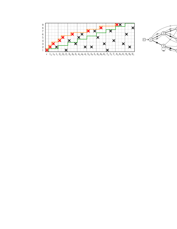
Figure 2. Left: a tableau with $n=9$ and $k=3$. The backbone part is in red. This tableau is valid because the red entries are monotonic (as shown by the orange profile), and $k$-Dyck because they are all on the left of the green staircase line. Right: the associated $k$-map. Backbone edges, corresponding to the breadth-first search tree, are thick, and wiring edges are in gray.

For a fixed integer $k$, when $M=N(n,k)=kn+1$, we have a special subfamily of tableaux in $\mathcal{T}[N\times n]$. A tableau is $k$-Dyck if $x_{T}(\ell)\leq k(\ell-1)+1$, i.e. if the backbone cells lie above the line of slope $1/k$ containing the origin of the grid. A small example of $k$-Dyck tableau is shown in Figure 2.

There exists a canonical bijection between $k$-Dyck tableaux and transition structures $\Delta$ of accessible deterministic complete automata. It suffices to associate the indices $(1,2,\ldots,n)$ of the states to the rows of the tableaux, and the indices $(\epsilon,1_{1},\ldots,1_{k},\cdots,$ $n_{1},\ldots,n_{k})$ of the oriented edges of $\Delta$ to the columns. Then, for $x=i_{\alpha}$, the entry $(x,y)$ is marked in $T$ if and only if $\delta_{\alpha}(i)=y$, and it is part of the backbone if and only if it is part of the breadth-first search tree on $\Delta$ started at the initial state.

Given a function $\hat{f}(y):[n]\to[M]$, consider the restriction of the set $\mathcal{T}[M\times n]$ to tableaux $T$ in which the backbone function $x_{T}(y)$ is dominated by $\hat{f}$, i.e., such that $x_{T}(y)\leq\hat{f}(y)$ for all $1\leq y\leq n$. Call $\mathcal{T}[M\times n;\hat{f}]$ this set. Our $k$-Dyck tableaux correspond to the special case $\mathcal{T}[N\times n;\hat{f}^{\varnothing}]$, with $\hat{f}^{\varnothing}(y):=N-k(n-y+1)$. A required technical lemma, that we state without proof, is the following

Proposition 4.2.

Take an integer $n$, $N=\mathcal{O}(n)$, $B=\mathcal{O}(1)$, and $\ell\gg\sqrt{n}$. Let $M=N-B$, and take a function $\hat{f}$ such that $\hat{f}(y)=\hat{f}^{\varnothing}(y)$ for all $y\leq\ell$, $\hat{f}(y)=\hat{f}^{\varnothing}(y)-B$ for all $y\geq n-\ell$, and $\hat{f}^{\varnothing}(y)-B\leq\hat{f}(y)\leq\hat{f}^{\varnothing}(y)$ for all $y$. Then

$$\frac{\big{|}cT[M\times n;\hat{f}]\big{|}}{\big{|}cT[M\times n]\big{|}}-\frac{\big{|}cT[N\times n;\hat{f}^{\varnothing}]\big{|}}{\big{|}cT[N\times n]\big{|}}=o(1)\,.$$ (15)

With these tools at hand, we are now ready to prove Proposition 3.2.

Proof of Proposition 3.2. Given three distinct states $i$, $j$, $h$, with $i<j<h$, call $\mathcal{M}_{ijh}(T)$ the event that in the tableau $T$ there is a three-state motif on states $\{i,j,h\}$ and $\{\ell_{\alpha}\}$, for some $\ell_{\alpha}$’s. Similarly, given $2r$ distinct states $\{(i_{a},j_{a})\}_{1\leq a\leq r}$, with $i_{a}<j_{a}$ and $j_{a}<j_{a+1}$, call $\mathcal{M}_{(i_{1},j_{1};\ldots;i_{r},j_{r})}(T)$ the event that in the tableau $T$ there is a $r$-uple of $M$-motifs, such that the $a$-th motif has states $i_{a}$, $j_{a}$, and $\{\ell_{\alpha}^{a}\}$, for some $\ell_{\alpha}^{a}$’s. Proposition 3.2 consists in evaluating the two quantities

$$\sum_{i<j<h}\mathbb{E}{}[\negthinspace[{\mathcal{M}_{ijh}}]\negthinspace]_{\mathcal{T}[N\times n;\hat{f}^{\varnothing}]}\,; \sum_{(i_{1},j_{1};\ldots;i_{r},j_{r})}\mathbb{E}{}[\negthinspace[{\mathcal{M}_{(i_{1},j_{1};\ldots;i_{r},j_{r})}}]\negthinspace]_{\mathcal{T}[N\times n;\hat{f}^{\varnothing}]}\,.$$ (16)

We now make a crucial remark: given a backbone structure $B$, the average over all possible completions of the indicator variables $[\negthinspace[{\mathcal{M}_{ijh}}]\negthinspace]$ (respectively $[\negthinspace[{\mathcal{M}_{(i_{1},j_{1};\ldots;i_{r},j_{r})}}]\negthinspace]$) is zero if any column of index in the set $C=\{k(j-1)+1+\alpha,k(h-1)+1+\alpha\}_{1\leq\alpha\leq k}$ has a red mark (respectively, in the set $C=\{k(j_{a}-1)+1+\alpha\}_{1\leq a\leq r;1\leq\alpha\leq k}$), otherwise, it is $\prod_{i\in C}y_{i}^{-1}$, where $y_{i}$ is the height of the backbone profile at column $i$. As a consequence, backbone structures contributing to the quantities in (16), weighted with the factor $\mu({\bm{c}})\prod_{i\in C}y_{i}^{-1}$, correspond to generic backbone structures, weighted with the factor $\mu({\bm{c}})$, over $(N-kr)\times n$ tableaux. The correspondence is done by just erasing the columns in $C$. The function $\hat{f}$ is modified accordingly. Define

$$\hat{f}^{i_{1},\ldots,i_{r}}(y)=\hat{f}^{\varnothing}(y)-k\sum_{a=1}^{r}[\negthinspace[{y\geq j_{a}}]\negthinspace]\,.$$ (17)

Then, the precise statement of the remark above is

$$\mathbb{E}{}[\negthinspace[{\mathcal{M}_{ijh}}]\negthinspace]_{\mathcal{T}[N\times n;\hat{f}^{\varnothing}]} =\frac{\big{|}\mathcal{T}[(N-2k)\times n;\hat{f}^{j,h}]\big{|}}{\big{|}\mathcal{T}[N\times n;\hat{f}^{\varnothing}]\big{|}}\,;$$ (18)

$$\mathbb{E}{}[\negthinspace[{\mathcal{M}_{(i_{1},j_{1};\ldots;i_{r},j_{r})}}]\negthinspace]_{\mathcal{T}[N\times n;\hat{f}^{\varnothing}]} =\frac{\big{|}\mathcal{T}[(N-kr)\times n;\hat{f}^{j_{1},\ldots,j_{r}}]\big{|}}{\big{|}\mathcal{T}[N\times n;\hat{f}^{\varnothing}]\big{|}}\,.$$ (19)

Thus, the right-hand side of (18) is just the special case $r=2$ of (19). Of course we have

$$\frac{\big{|}\mathcal{T}[(N-kr)\times n;\hat{f}^{j_{1},\ldots,j_{r}}]\big{|}}{\big{|}\mathcal{T}[N\times n;\hat{f}^{\varnothing}]\big{|}}=\frac{\frac{\big{|}\mathcal{T}[(N-kr)\times n;\hat{f}^{j_{1},\ldots,j_{r}}]\big{|}}{\big{|}\mathcal{T}[(N-kr)\times n]\big{|}}}{\frac{\big{|}\mathcal{T}[N\times n;\hat{f}^{\varnothing}]\big{|}}{\big{|}\mathcal{T}[N\times n]\big{|}}}\;\frac{\big{|}\mathcal{T}[(N-kr)\times n]\big{|}}{\big{|}\mathcal{T}[N\times n]\big{|}}\,.$$ (20)

We can apply Proposition 4.1 to the rightmost ratio. Then, if the $j_{a}$’s are within the range for application of Proposition 4.2, we can also simplify the leftmost ratio, to get

$$\mathbb{E}{}[\negthinspace[{\mathcal{M}_{ijh}}]\negthinspace]_{\mathcal{T}[N\times n;\hat{f}^{\varnothing}]} \simeq\left(\frac{\omega_{k}}{n}\right)^{2k}\,;$$ (21)

$$\mathbb{E}{}[\negthinspace[{\mathcal{M}_{(i_{1},j_{1};\ldots;i_{r},j_{r})}}]\negthinspace]_{\mathcal{T}[N\times n;\hat{f}^{\varnothing}]} \simeq\left(\frac{\omega_{k}}{n}\right)^{kr}\,.$$ (22)

As in Proposition 4.2 we just asked for $\ell\gg\sqrt{n}$, which is compatible with $\ell\ll n$, the fraction of $2r$-uples $(i_{1},j_{1};\ldots;i_{r},j_{r})$ such that some $j_{a}$’s are out of range is subleading, and, using the reasonings at the beginning of Section 3, the corresponding contribution can be included in $P_{\rm confl}$.

Then, the straightforward calculation of the number of triplets $(i,j,h)$, and $2r$-uplets $\{(i_{a},j_{a})\}_{1\leq a\leq r}$, at leading order in $n$, allows to conclude. ∎

5. Algorithmic consequences

The results obtained in this paper open new possibilities for the study in average of the properties of regular languages, and of the average-case complexity of algorithms applied to minimal automata. In this section we mention just a few among these consequences.

Corollary 1.

Minimal automata with $n$ states over a $k$-letter alphabet can be randomly generated with $\mathcal{O}(n^{3/2})$ average complexity, using Boltzmann samplers.

The random generator for complete deterministic accessible automata given in [4] is based on a Boltzmann sampler [9], its average complexity is $\mathcal{O}(n^{3/2})$. As from Theorem 2.1 there is a constant proportion of minimal automata amongst accessible ones, the rejection method can be efficiently applied to randomly generate a minimal automaton. Note that such a generator has already been implemented in [2], though there were no theoretical result on the efficiency of this algorithm at that time.

Corollary 2.

For the uniform distribution on complete deterministic accessible automata, the average complexity of Moore’s state minimization algorithm is $\Theta(n\log\log n)$.

Proof 5.1.

The average complexity of Moore’s state minimization algorithm for the uniform distribution on n-state deterministic automata over a finite alphabet is $\mathcal{O}(n\log\log n)$ [8]. The upper bound for accessible automata is then obtained studying the size of the accessible part of a $k$-random map [7, 19]. Moreover from [3] the lower bound of Moore’s algorithm applied on minimal automata with $n$ states is $\Omega(n\log\log n)$. Using Theorem 2.1, this is also a lower bound for complete deterministic accessible automata.

Corollary 3.

For the uniform distribution on complete deterministic accessible automata, there exists a family of implementations of Hopcroft’s state minimization algorithm whose average complexity is $\mathcal{O}(n\log\log n)$.

From [8] a family of implementations of Hopcroft’s state minimization algorithm are always faster than Moore’s algorithm. The result follows from Corollary 2. In [5] the lower bound on the algorithm is proved to be $\mathcal{O}(n\log n)$ for any implementation. Though it is still unknown whether there exists an implementation whose average complexity is $\Theta(n)$.

Appendix A Details of the proof of Proposition 3.3

We perform here a detailed derivation of equation (11), that has been omitted in the body of the paper. In this section we use the notation $(n)_{c}\equiv n(n-1)\cdots(n-c+1)$.

Thus we have the simultaneous breadth-first tree exploration started at a pair $\{i,j\}$ of states, in which we do not follow the leaf nodes, i.e., those nodes where, in one or both of the two trees, there is a state already visited by the exploration.

This exploration is finite (the number of steps, $L_{ij}$, being bounded by $\sim n$), as we cannot indefinitely visit new states. A string $\tau^{(ij)}$ in $\{0,1,2\}^{L_{ij}}$ is associated to this procedure, (just use $\tau\equiv\tau^{(ij)}$ when no confusion arises), with $\tau_{s}$ corresponding to the number of states already visited, among the two involved with the $s$-th step.

The exclusion of sink and quasi-sink motifs leads to the fact that, among $\{\tau_{1},\ldots,\tau_{k}\}$ there must be at least a value zero. Say $\alpha^{*}_{ij}$ is the first lexicographc letter with this property. A further consequence is that we have at least $k+1$ non-zero entries $\tau_{s}$, for $1\leq s\leq L_{ij}$.

Recognize that the sequence $(v_{1},v_{2},\ldots)$ is exactly the ordered sequence of positions $s$ at which $\tau_{s}>0$. Call $|\tau|_{s}=\sum_{t\leq s}\tau_{t}$.

We now fix $v\ll n/2$, and $h=\mathcal{O}(1)$. The probability for the $h$-uple $(v_{1},\ldots,v_{h})$ is

$$P(v_{1},\ldots,v_{h}) =\sum_{\{\tau_{v_{j}}\}\in\{1,2\}^{h}}\frac{1}{n^{2v_{h}}}(n)_{2v_{h}-|\tau|_{v_{h}}}\bigg{(}\prod_{j=1}^{h}W_{j}\bigg{)}\,;$$ (23)

$$W_{j} =\left\{\begin{array}[]{ll}2(v_{j}-|\tau|_{v_{j}-1})+1&\tau_{v_{j}}=1\\ (v_{j}-|\tau|_{v_{j}-1})^{2}&\tau_{v_{j}}=2\end{array}\right.$$ (26)

We can bound from above the probability that $v_{h}\leq v$.

$$\begin{split}\mathrm{prob}(v_{h}\leq v)&=\!\!\sum_{\begin{subarray}{c}(v_{1},\ldots,v_{h})\\ v_{h}\leq v\end{subarray}}\!\!\!P(v_{1},\ldots,v_{h})\leq\!\!\sum_{\begin{subarray}{c}(v_{1},\ldots,v_{h})\\ v_{h}\leq v\end{subarray}}\sum_{\{\tau_{v_{j}}\}\in\{1,2\}^{h}}\!\!\!\frac{(n)_{2v_{h}}}{n^{2v_{h}}}(n-2v)^{-|\tau|_{v_{h}}}\bigg{(}\prod_{j=1}^{h}W_{j}\bigg{)}\\ &\leq\!\!\sum_{\begin{subarray}{c}(v_{1},\ldots,v_{h})\\ v_{h}\leq v\end{subarray}}\sum_{\{\tau_{v_{j}}\}\in\{1,2\}^{h}}\prod_{j=1}^{h}\left(\frac{2v_{j}+1}{n-2v}\right)^{\tau_{v_{j}}}\leq\!\!\sum_{\begin{subarray}{c}(v_{1},\ldots,v_{h})\\ v_{h}\leq v\end{subarray}}\!\!\left(n-2v\right)^{-h}\prod_{j=1}^{h}(2v_{j}+2)\,;\end{split}$$ (27)

where in the last passage we used the fact that $\frac{1}{n-2v}<1$. Now we use the fact that, for $f(v_{1},\ldots,v_{h})$ a positive function,

$$\sum_{\begin{subarray}{c}v_{1}<\ldots<v_{h}\\ v_{h}\leq v\end{subarray}}f(v_{1},\ldots,v_{h})\leq\frac{1}{h!}\sum_{\begin{subarray}{c}v_{1},\ldots,v_{h}\\ v_{j}\leq v\end{subarray}}f(v_{1},\ldots,v_{h})$$ (28)

to get

$$\begin{split}\mathrm{prob}(v_{h}\leq v)&\leq\frac{\left(n-2v\right)^{-h}}{h!}\sum_{\begin{subarray}{c}v_{1},\ldots,v_{h}\\ v_{j}\leq v\end{subarray}}\prod_{j=1}^{h}(2v_{j}+2)=\frac{1}{h!}\left(\frac{v(v+1)}{n-2v}\right)^{h}\,.\end{split}$$ (29)

This gives the claim in equation (11).

Appendix B Some statistical properties of tableaux

We investigate here some statistical properties of tableaux and $k$-Dyck tableaux, concerning the limit distribution of the marks, and its fluctuations. These results are interesting per se, and, at the aims ofthis paper, will be instrumental to determine ratios of cardinalities of various sets of tableaux, that, in turns, are used in the proof of Proposition 3.2.

Associate to the backbone part $B_{T}$ of a tableau $T$ the sequence ${\bm{c}}=(c_{1},c_{2},\ldots,c_{n})$, as $c_{y}=x_{T}(y+1)-x_{T}(y)-1$ (let conventionally $x_{T}(0)=0$ and $x_{T}(n+1)\equiv kn+2$). The $c_{y}$’s are non-negative integers, related to the incremental steps in the tableau shape $x_{T}(y)$.

Call $\mu({\bm{c}})$ the number of tableaux having the given backbone ${\bm{c}}$. This quantity is easily determined. For ${\bm{c}}\in\mathbb{N}^{M}$, $\mu({\bm{c}})=0$ if $\sum_{y}c_{y}\neq(k-1)n+1$, and otherwise

$$\mu({\bm{c}})=\prod_{y=1}^{n}y^{c_{y}}\,.$$ (30)

The property of a tableau $T=(B_{T},W_{T})$ of being $k$-Dyck depends only on the backbone part $B_{T}$, and we can naturally talk of $k$-Dyck backbones. The factorization above still holds for $k$-Dyck tableaux, if it is intended that $\sum_{B}$ is restricted to $k$-Dyck backbones.

The backbone profile has a definite limit shape for large $n$, that we can readily determine. Define the function $f_{\kappa}(y):[0,1]\to[0,k]$

$$f_{\kappa}(y)=\lim_{n\to\infty}\frac{1}{n}\mathbb{E}{\,x_{T}(ny)}$$ (31)

where the average is taken w.r.t. the uniform measure on $\mathcal{T}[(\lfloor\kappa n\rfloor+1)\times n]$. Provided that we have pointwise convergence to a differentiable function (as we will see, this is the case here), this function is translated into marginals on the sequence ${\bm{c}}$, through $\frac{{\rm d}f_{\kappa}(y)}{{\rm d}y}=1+\lim_{n\to\infty}\mathbb{E}{\,c_{yn}}$.

We deal with the overall constraint by introducing a Lagrange multiplier, associated to the horizontal width of the tableau, (to be tuned later on in order to have concentration on the appropriate width value $\lfloor\kappa n\rfloor+1$). The resulting measure is

$$\mu_{\omega}({\bm{c}})=\prod_{y=1}^{n}(\omega y)^{c_{y}}\,.$$ (32)

Now the variables $c_{y}$ are independent geometric variables, with parameter $\rho=\omega y$ (i.e., $p_{y}(c)=(1-\rho)\rho^{c}$). Average and variance are given by

$$\left\langle{c_{y}}\right\rangle_{\omega} =\frac{\omega y}{1-\omega y}\,; \left\langle{c_{y}^{2}}\right\rangle_{\omega}-\left\langle{c_{y}}\right\rangle_{\omega}^{2} =\frac{\omega y}{(1-\omega y)^{2}}\,.$$ (33)

The value of $\omega$ is determined by the equation $\sum_{y=1}^{n}\frac{\omega y}{1-\omega y}=(\kappa-1)n+1$, that is, in the large $n$ limit,

$$\int_{0}^{n}\!\mathrm{d}{y}\,\frac{\omega y}{1-\omega y}=(\kappa-1)n+\mathcal{O}(1)\,.$$ (34)

Through the scaling $y\to y/n$, $\omega\to\omega n$ we can extract the leading contribution $\int_{0}^{1}\!\mathrm{d}{y}\,\frac{\omega y}{1-\omega y}=\kappa-1$, and, as we have

$$\int_{y=0}^{Y}\!\mathrm{d}{y}\,\frac{\omega y}{1-\omega y}=-Y-\frac{\ln(1-\omega Y)}{\omega}\,,$$ (35)

we get that value $\omega_{\kappa}$ for the multiplier is the root in the interval $(0,1)$ of the transcendental equation

$$\kappa=-\frac{\ln(1-\omega)}{\omega}\,,$$ (36)

that is, the same constants defined in (3). Then, the limit curve is just deduced from (35) with $\omega=\omega_{\kappa}$:

$$f_{\kappa}(y)=-\frac{\ln(1-\omega_{\kappa}y)}{\omega_{\kappa}}\,.$$ (37)

Note that the derivative of $f_{\kappa}(y)$ at $y=0$ and $y=1$ are $f^{\prime}_{\kappa}(0)=1$ and $f^{\prime}_{\kappa}(1)=\frac{1}{1-\omega_{\kappa}}$, which are respectively smaller and larger than $\kappa$, for any $\kappa>1$ real. More generally, $\big{(}f^{\prime}_{\kappa}(y)\big{)}^{-1}=1-\omega_{\kappa}y$ is the density of backbone marks around $x=f_{\kappa}(y)$. As every column is marked, either in red or in black, the density of black marks around $x=f_{\kappa}(y)$ is $\omega_{\kappa}y$. As the position of a black mark in a given column is chosen uniformly in the range $\{1,\ldots,y\}$, the probability of putting a black mark in a given position $(x,y)$, provided that $x>f_{\kappa}(y)$, is $\omega_{\kappa}/n$, notably regardless of $x$ and $y$.

A further useful property of the backbone is the calculation of the variance, in the system with the Lagrange multiplier (and thus without the constraint $\sum_{y}c_{y}=(k-1)n+1$), which is given by the integral

$$S(Y)=\int_{0}^{Y}\!\mathrm{d}{y}\,\frac{\omega y}{(1-\omega y)^{2}}=\frac{Y}{1-\omega Y}+\frac{\ln(1-\omega Y)}{\omega}\,.$$ (38)

Through the Central Limit Theorem we can deduce from this expression the asymptotic probability for fluctuations from the limit shape. For a given row $y$, such that $y$, $n-y\gg 1$, the probability of having $x_{T}(y)=\lfloor nf_{\kappa}(y)\rfloor+\xi$ is approximatively (using here the variance function (38))

$$p^{\rm bridge}_{n,y}(\xi) =\frac{1}{\sqrt{2\pi s}}\exp\left[-\frac{\xi^{2}}{2s}\right]\,; s=n\frac{S(1)}{S(y/n)(S(1)-S(y/n))}\,.$$ (39)

This is of course only the case $r=1$ of the basic formulas for the $r$-point joint distribution in an inhomogeneous Wiener Process $x(t)$, derived from the continuum limit of the sum of independent random variables with variance $S(t)$, as in our case (see e.g. [17, sec. 5.6]). However, this formula will be sufficient at our present purposes.

We have now all the ingredients to prove Proposition 4.2.

Proof of Proposition 4.2. We start by comparing different functions $\hat{f}$ satisfying the constraint, at a fixed value $M$. Remark that any two such functions $\hat{f}_{1}$, $\hat{f}_{2}$ differ by a number of cells bounded by $Bn$, and that, if $\hat{f}_{1}(y)\leq\hat{f}_{2}(y)$ for all $y$, $\big{|}cT[M\times n;\hat{f}_{1}]\big{|}\leq\big{|}cT[M\times n;\hat{f}_{2}]\big{|}$. Thus, by telescoping, up to a factor $Bn$, it suffices to estimate the quantity

$$\frac{\big{|}cT[M\times n;\hat{f}_{2}]\big{|}-\big{|}cT[M\times n;\hat{f}_{1}]\big{|}}{\big{|}cT[M\times n]\big{|}}$$

for a pair of functions $\hat{f}_{1}$, $\hat{f}_{2}$ differing by a single cell in the position $(x,y)$. This quantity is positive at sight.

Note that the constraint on functions $\hat{f}$ forces $y$, $n-y\gg\sqrt{n}$. Thus, the use of (39) (based on use of the Central Limit Theorem) is legitimate, and we have

$$\begin{split}\frac{\big{|}cT[M\times n;\hat{f}_{2}]\big{|}-\big{|}cT[M\times n;\hat{f}_{1}]\big{|}}{\big{|}cT[M\times n]\big{|}}&\sim p^{\rm bridge}_{n,y}(ky-nf(y)+\mathcal{O}(1))\\ &\sim\exp\left(-\mathcal{O}\left(\genfrac{}{}{0.25pt}{1}{\min(y,n-y)^{2}}{n}\right)\right)\,,\end{split}$$ (40)

where the constant is positive at sight, and could be determined from the expressions (38) giving $S(y/n)$ and $S(1)-S(y/n)$ (which are of order 1), and the quantity $ky-nf_{k}(y)$ (with $f_{k}(y)$ as in (37)), which is of order $\min(y,n-y)$. The precise value is accessible with some calculation, but irrelevant at our purposes.

Now that we determined that all functions $\hat{f}$ in the appropriate range produce the same ratio, up to an absolute error which is exponentially small, we can evaluate this ratio, for a reference $\hat{f}$ of our choice. We choose, for any value $a$ such that both $a$ and $n-a$ are of order $n$,

$$\hat{f}_{a}(y)=\left\{\begin{array}[]{ll}\hat{f}^{\varnothing}(y)&y<n-a\\ \hat{f}^{\varnothing}(y)-B&y\geq n-a\end{array}\right.$$ (41)

For a tableau $T$, call $M^{\prime}$ the value such that $x_{T}(n-a)=M^{\prime}<M-k(a+1)$, the latter inequality being forced by the constraint $x_{T}(y)\leq\hat{f}(y)$. We can thus express the ratio $\big{|}cT[M\times n;\hat{f}]\big{|}/\big{|}cT[M\times n]\big{|}$ in the form

$$\begin{split}\frac{\big{|}cT[M\times n;\hat{f}]\big{|}}{\big{|}cT[M\times n]\big{|}}&=\frac{1}{\displaystyle{\sum_{{\bm{c}}}\mu_{\omega}({\bm{c}})[\negthinspace[{|{\bm{c}}|=M-n}]\negthinspace]}}\sum_{M^{\prime}<M-k(a+1)}\sum_{{\bm{c}}}\mu_{\omega}({\bm{c}})[\negthinspace[{|{\bm{c}}|=M-n}]\negthinspace]\\ &\qquad\times[\negthinspace[{x_{T}(n-a)=M^{\prime}}]\negthinspace][\negthinspace[{x_{T}(y)\leq\hat{f}(y)}]\negthinspace]_{y>n-a}[\negthinspace[{x_{T}(y)\leq\hat{f}(y)}]\negthinspace]_{y<n-a}\,.\end{split}$$ (42)

The marginalisation on the value of $M^{\prime}$ makes the two event $[\negthinspace[{x_{T}(y)\leq\hat{f}(y)}]\negthinspace]_{y>n-a}$ and $[\negthinspace[{x_{T}(y)\leq\hat{f}(y)}]\negthinspace]_{y<n-a}$ independent, and in fact the second one depends only on $n-a$ and $M^{\prime}$, and the first one only on $n$, $a$ and $M-M^{\prime}$ (not on $B$). Equivalently, as $N=kn+1=M-B$, we can use $n$, $a$ and $M^{\prime}-B$ as independent parameters, i.e.,

$$\begin{split}\frac{\big{|}cT[M\times n;\hat{f}]\big{|}}{\big{|}cT[M\times n]\big{|}}&=\sum_{M^{\prime}<M-k(a+1)}p(M^{\prime})\;p^{+}_{n,a}(M^{\prime}-B)\;p^{-}_{a}(M^{\prime})\,.\end{split}$$ (43)

where $p(M^{\prime})$ is nothing but $p^{\rm bridge}_{n,n-a}(M^{\prime}-nf(y))$, and corresponds to the expectation of $[\negthinspace[{x_{T}(n-a)=M^{\prime}}]\negthinspace]$ alone. From equation (39) we know that the leading contribution to $p(M^{\prime})$ is well-approximated by a Gaussian, with mean and variance

$$\mathbb{E}{}\left(\genfrac{}{}{0.25pt}{1}{M^{\prime}}{M}\right) =f\left(\genfrac{}{}{0.25pt}{1}{n-a}{n}\right)\,; \mathbb{E}{}(M^{\prime})^{2}-(\mathbb{E}{}M^{\prime})^{2}=M\frac{S(1)}{S(\frac{n-a}{n})\big{(}S(1)-S(\frac{n-a}{n})\big{)}}\,,$$ (44)

where, as $(M-1)/n=k+\mathcal{O}(1/n)$, up to subleading corrections we can use the parameters $k$ and $\omega_{k}$ in the determination of $f(y)$ and $S(y)$. Similarly, as the width of the Gaussian is of order $\sqrt{N}$, up to subleading corrections we can replace $p(M^{\prime})$ by $p(M^{\prime}-B)$, and write, after a translation,

$$\begin{split}\frac{\big{|}cT[M\times n;\hat{f}]\big{|}}{\big{|}cT[M\times n]\big{|}}&=\sum_{M^{\prime}<N-k(a+1)}p(M^{\prime})\;p^{+}_{n,a}(M^{\prime})\;p^{-}_{a}(M^{\prime}+B)\,.\end{split}$$ (45)

The expression analogous to (45), for $M=N$, reads

$$\begin{split}\frac{\big{|}cT[N\times n;\hat{f}]\big{|}}{\big{|}cT[N\times n]\big{|}}&=\sum_{M^{\prime}<N-k(a+1)}p(M^{\prime})\;p^{+}_{n,a}(M^{\prime})\;p^{-}_{a}(M^{\prime})\,.\end{split}$$ (46)

As the Korshunov constant is of order $1$ for all $k>1$, the values of the Gaussian $p(M^{\prime})$ are of order $1/\sqrt{N}$ at the maximum, and the functions $p^{+}_{n,a}(M^{\prime})$ and $p^{-}_{a}(M^{\prime})$ are (respectively decreasing and increasing) monotonic in $M^{\prime}$, we have that these functions must be of order 1 in the region relevant for $p(M^{\prime})$. Actually, in this region we even have $p^{-}_{a}(M^{\prime})=1-o(1)$ (see [4, Lemma 13]), and in particular, as a corollary, $p^{-}_{a}(M^{\prime})$ is smooth possibly up to small corrections. Then, the comparison of (45) and (46) allows to conclude. ∎

References

- [1] N. Alon and J. Spencer. The Probabilistic Method. 2nd ed., John Wiley, 2000.
- [2] F. Bassino, J. David and C. Nicaud. REGAL: A library to randomly and exhaustively generate automata. In J. Holub and J. Zdárek eds, 12th International Conference Implementation and Application of Automata (CIAA 2007), LNCS 4783, 303–305. Springer, 2007.
- [3] F. Bassino, J. David and C. Nicaud. Average-case analysis of Moore’s state minimization algorithm. Algorithmica, to appear. Available at http://lipn.fr/bassino/publications.html
- [4] F. Bassino and C. Nicaud. Enumeration and random generation of accessible automata. Theor. Comput. Sci., 381 86–104, 2007.
- [5] J. Berstel, L. Boasson and O. Carton. Continuant polynomials and worst-case behavior of Hopcroft’s minimization algorithm. Theor. Comput. Sci., 410 2811–2822, 2009.
- [6] J.R. Buchi. Weak second-order arithmetic and finite automata. Math. Logic Quart., 6 66–92, 1960.
- [7] A. Carayol and C. Nicaud. Distribution of the number of accessible states in a random deterministic automaton Submitted to STACS 2012.
- [8] J. David. Average complexity of Moore’s and Hopcroft’s algorithms. Theor. Comput. Sci. to appear. Available at http://www-lipn.univ-paris13.fr/david/
- [9] P. Duchon, P. Flajolet, G. Louchard and G. Schaeffer. Boltzmann Samplers for the Random Generation of Combinatorial Structures. In Combinatorics, Probability, and Computing, Special issue on Analysis of Algorithms 13 577–625, 2004.
- [10] P. Flajolet and R. Sedgewick. Analytic Combinatorics. Cambridge Univ. Press, 2009.
- [11] I.J. Good, An Asymptotic Formula for the Differences of the Powers at Zero. Ann. Math. Stat. 32 249–256, 1961.
- [12] R.L. Graham, D.E. Knuth and O. Patashnik. Concrete Mathematics: A Foundation for Computer Science. 2nd ed., Addison-Wesley, Reading, Mass., 1994.
- [13] F. Harary. Unsolved problems in the enumeration of graphs. Publ. Math. Inst. Hungar. Acad. Sci., 5 63–95, 1960.
- [14] M.A. Harrison. A census of finite automata, Canad. Journ. of Math., 17 100–113, 1965.
- [15] J.E. Hopcroft and J.D. Ullman. Introduction to Automata Theory, Languages and Computation. Addison-Wesley, 1979.
- [16] J.E. Hopcroft. An algorithm for minimizing states in a finite automaton. Technical report, Stanford CA, USA, 1971.
- [17] R. Iranpour and P. Chacon. Basic Stochastic Processes: The Mark Kac Lectures. Macmillan Publ. Co., 1988.
- [18] S. Kleene. Representation of Events in Nerve Nets and Finite Automata. In C. Shannon and J. Mccarthy eds., Automata Studies, 3–42. Princeton University Press, 1956.
- [19] A.D. Korshunov. Enumeration of finite automata. Problemy Kibernetiki, 34 5–82, 1978. In Russian.
- [20] A.D. Korshunov. On the number of non-isomorphic strongly connected finite automata. Journal of Information Processing and Cybernetics, 9 459–462, 1986.
- [21] E. Lebensztayn. On the asymptotic enumeration of accessible automata. Discr. Math. Theor. Comp. Science 12 75–80, 2010
- [22] V.A. Liskovets. Enumeration of non-isomorphic strongly connected automata, Vesci Akad. Navuk BSSR, Ser. Fiz.-Mat. Navuk, 3 26–30, 1971. In Russian.
- [23] V.A. Liskovets. Exact enumeration of acyclic automata. In FPSAC’03, K. Eriksson, A. Björner and S. Linusson eds. Available at http://www.i3s.unice.fr/fpsac/FPSAC03/ARTICLES/5.pdf.
- [24] E.F. Moore. Gedanken experiments on sequential machines. In Automata Studies, Princeton Univ., 129–153, 1956.
- [25] A. Nerode. Linear automaton transformations. Proc. of the American Math. Society, 9 541–544, 1958.
- [26] C. Nicaud. Average state complexity of operations on unary automata. In 24th International Symposium on Mathematical Foundations of Computer Science (MFCS 1999), 231–240, 1999.
- [27] R. Robinson, Counting strongly connected finite automata, In Graph theory with Applications to Algorithms and Computer Science, Y. Alavi et al. eds., Wiley, 671–685, 1985.
- [28] J. Sakarovitch, Eléments de théorie des automates, Vuibert, 2003. English translation: Elements of Automata Theory, Cambridge Univ. Press, to appear.
- [29] S. Yu, Q. Zhuang and K. Salomaa, The state complexities of some basic operations on regular languages, Theoret. Comput. Sci., 125 315–328, 1994.