Intracluster medium of the merging cluster Abell 3395

Abstract

We present a detailed imaging and spectral analysis of the merging environment of the bimodal cluster A3395 using X-ray and radio observations. X-ray images of the cluster show five main constituents of diffuse emission : A3395 NE, A3395 SW, A3395 NW, A3395 W, and a filament connecting NE to W. X-ray surface-brightness profiles of the cluster did not show any shock fronts in the cluster. Temperature and entropy maps show high temperature and high entropy regions in the W, the NW, the filament and between the NE and SW subclusters. The NE, SW and W components have X-ray bolometric luminosities similar to those of rich clusters of galaxies but have relatively higher temperatures. Similarly, the NW component has X-ray bolometric luminosity similar to that of isolated groups but with much higher temperature. It is, therefore, possible that all the components of the cluster have been heated by the ongoing mergers. The NE subcluster is the most massive and luminous constituent and other subclusters are found to be gravitationally bound to it. The W component is most probably either a clump of gas stripped off the SW due to ram pressure or a separate subcluster that has merged or is merging with the SW. No X-ray cavities are seen associated with the Wide Angle Tailed (WAT) radio source near the centre of the SW subcluster. Minimum energy pressure in the radio emission-peaks of the WAT galaxy is comparable with the external thermal pressure. The radio spectrum of the WAT suggests a spectral age of $\sim$∼10Myr.

1 Introduction

Clusters of galaxies, the largest gravitationally-bound structures, are believed to form hierarchically in a sequence of cosmic structure formation where smaller groups of galaxies merge to form larger and richer systems (Geller & Beers 1982; Dressler & Shectman 1988; Girardi et al. 1997; Kriessler & Beers 1997; Jones & Forman 1999; Schuecker et al. 2001; Burgett et al. 2004). The intra-group or intra-cluster medium (ICM) of these clusters contains a hot (T$\sim 10^{7}-10^{8}$K) and tenuous (n$\sim 10^{-3}$ cm^-3) plasma which emits in X-rays mainly through bremsstrahlung and line emission (Kellogg et al. 1972; Mitchell et al. 1979; also see reviews by Sarazin 1988; McNamara & Nulsen 2007). Although many rich clusters show smooth X-ray surface-brightness distributions with a central peak, a large fraction (at least, $\sim$30% (Forman & Jones 1990) or even up to $\sim$40%-60% (Jones & Forman 1992, 1999; Schuecker et al. 2001)) shows double or multiple peaks in their X-ray surface brightness maps. As X-ray surface-brightness is more sensitive to density than temperature these observations effectively show peaks in the density distribution of the ICM itself, which suggests the presence of subclusters or substructures which are possibly in the process of merging to form richer groups and clusters of galaxies (e.g. Nakamura et al. 1995). Presence of large inhomogeneities in the X-ray temperature of the ICM (greater than a few keV) on scales less than 0.5 Mpc provides additional observational evidence of mergers (Roettiger et al. 1996). As dynamical evolution rapidly removes substructures, their existence proves that such clusters are dynamically young systems (Flin 2003).

For studies of cosmology and the formation and evolution of large-scale structures, it is important to study the physical properties of clusters of galaxies containing sub-groups which are young and in the process of merging. Mergers of subgroups can produce shocks, bulk gas flows and turbulence in the ICM, and can disrupt cooling flows as has been seen in many clusters (see Fabian 1994; Markevitch & Vikhlinin 2007; Owers et al. 2011; Maurogordato et al. 2011). Mergers may also cause metal enrichment of the ICM through enhanced ram-pressure stripping during mergers (Domainko et al. 2005), thereby affecting the evolution of the galaxies and the ICM. Subclustering information has also been used for estimating cosmological parameters such as the density parameter $\Omega_{0}$ (Richstone et al. 1992; Kauffmann & White 1993, Angrick & Bartelmann 2011).

At radio wavelengths, besides the diffuse emission which may be in the form of halos and relics, the tailed radio sources associated with individual galaxies can provide further insights towards understanding these systems. For example, the Wide Angle Tail (WAT) galaxies are usually associated with the dominant galaxy in a group or a cluster, with the jets flaring into tails of emission which can extend to over a Mpc in size (e.g. Roettiger et al. 1996; Douglass et al. 2008; Mao et al. 2010). Their relatively high luminosity, close to the upper range of the Fanaroff-Riley I sources, and large sizes make these good tracers of galaxy clusters at moderate and high redshifts (e.g. Blanton et al. 2003; Douglass et al. 2008). Since the dominant galaxies with which WATs are associated are likely to have at most small peculiar velocities, their jets are unlikely to be bent by ram pressure caused by the motion of the galaxy (Burns 1981; Eilek et al. 1984; O’Donoghue et al. 1990). Cluster mergers where relative velocities between the systems can exceed $\sim$1000 km s^-1, causing significant bulk motion of the ICM, have been invoked as the primary scenario for understanding the WAT structures (Eilek et al. 1984; Burns et al. 1994; Roettiger et al. 1996).

X-ray observatories, particularly Chandra and XMM-Newton, have brought to light new information leading to a more detailed understanding and new insights into the physical processes occurring in galaxy clusters (Weratschnig 2010). While Chandra with its unprecedented spatial resolution of 0.5^′′ can study small-scale phenomena such as cold fronts, merger shocks and AGN cavities, XMM-Newton with its larger collecting area and sensitivity can study clusters to a much farther extent and can detect fainter X-ray signals. Because of its large FOV of $\sim 30^{\prime}$ and moderate resolution (6^′′ FWHM), XMM-Newton can also study the nearby clusters very well.

We have chosen A3395 for a detailed study of its merging environment since it is a well-known bimodal merging cluster (Henriksen & Jones 1996; Markevitch et al. 1998; Donnelly et al. 2001; Flin & Krywult 2006) and it has been observed with XMM-Newton, Chandra and Australia Telescope Compact Array (ATCA).

The paper is organized as follows. Detailed information about A3395 and a summary of its earlier X-ray observations with the Roentgen Satellite (ROSAT) and the Advanced Satellite for Cosmology and Astrophysics (ASCA) and the previous radio observations are given in §2. The details of the recent X-ray and unpublished radio observations and their data analyses, are presented in §3. The results including the X-ray and radio morphology, X-ray surface brightness profiles, X-ray temperature, metallicity, density, entropy and pressure maps, mass, luminosity and cooling time estimates are provided in §4. A discussion of the results and the merging environment of A3395 is given in §5. A lambda cold dark matter cosmology with $H_{0}$ = 70 km s^-1 Mpc^-1 and $\Omega_{M}$ = 0.3 ($\Omega_{\Lambda}$ = 0.7) has been assumed, so that 1 arcsec corresponds to 0.96 kpc at z=0.0498, the redshift of the cluster.

2 A3395

Located nearby, at a distance of 211 Mpc and redshift of 0.0498, the positional coordinates of A3395 are : R.A.(J2000) $=06^{\rm h}27^{\rm m}31.1^{\rm s}$, Dec.(J2000)$=-54^{\rm d}23^{\prime}58^{\prime\prime}$ (l=262.9589^∘, b=-25.007^∘) (from Set of Identifications, Measurements, and Bibliography for Astronomical Database (SIMBAD)). A3395 is a regular cluster with 54 members (cluster members between m₃ (magnitude of $3^{\rm rd}$ brightest galaxy) and m₃+2) and richness class 1 (Abell, Corwin, & Olowin, 1989). It has a large extent with $r_{180}$ (radius within which mean density of the cluster equals 180 times the critical density at the redshift of the cluster) $=$ 34.6^′ (Markevitch et al. 1998) and hence can be studied with XMM-Newton very well.

A3395 has been observed previously in X-rays with the ROSAT Position Sensitive Proportional Counter (PSPC) by Henriksen & Jones (1996). They reported temperature of 2 to 4 keV for the cluster and calculated the cooling time for the cluster as $\sim 10$ Gyr, which is much larger than the time predicted for the cluster to fully merge. Hence, they suggested that either there are no cooling flows at the centre of the cluster or the cooling flows are disrupted by the merger. Markevitch et al. (1998) reanalyzed the ROSAT PSPC data and combined it with the analysis of ASCA observations. They found some evidence for the presence of shock-heated gas in the cluster and suggested that a collision between the two subclusters may be responsible for heating the gas. They calculated the emission-weighted gas temperature $T_{X}$ of A3395 (excluding cooling flow and other contaminating components) to be $4.8\pm 0.4$ keV. Donnelly et al. (2001) reanalyzed both the ROSAT PSPC and the ASCA data and reinforced the evidence for a merger in A3395, as they detected a rise in the gas temperature ($\sim 30\%$ above the average temperature) in the region between the two main subcluster components. By using Newtonian energy considerations Donnelly et al. proved that the system of the two subclusters is in a bound state and determined the virial masses of the two main subclusters (NE and SW) as $4.5^{+1.1}_{-0.9}\times 10^{14}\rm M_{\odot}$ and $3.1^{1.8}_{-1.4}\times 10^{14}\rm M_{\odot}$ respectively. Tittley & Henriksen (2001) report the presence of a group of lower redshift galaxies (z=0.048), at $\sim 12^{\prime}$ northwest from the centre of the galaxy distribution, which is elongated in the NW-SE direction. They found an increase in the X-ray emission from this group and classified this as the third component of X-ray emission viz., A3395 NW (centred at R.A.(J2000) $=06^{\rm h}26^{\rm m}35^{\rm s}$, Dec.(J2000)$=-54^{\rm d}20^{\prime}$). This is in addition to the two main X-ray peaks A3395 NE and A3395 SW, that coincide with subclusters, at slightly higher redshifts of 0.051 and 0.052 respectively. Using ASCA and wide field of view ROSAT observations, they also detected a filamentary structure that connects the clusters A3395 and A3391, shown by the presence of excess X-ray emission in a region between the two clusters and aligned with the distribution of galaxies.

A3395 has also been observed in radio with the Molonglo Cross Telescope at 408 MHz (Large et al. 1981) and with the Molonglo Observatory Synthesis Telescope (MOST) at 843 MHz (Jones & McAdam 1992; Burgess & Hunstead 2006). The observations showed a WAT inside the cluster. The cluster was also observed by ATCA at a frequency of 4.79 GHz (Gregorini et al. 1994). Reid (2000) used ATCA observations of this cluster at 1348 MHz and 2374 MHz, and detected eight radio sources of which five had optical counterparts. There are 2 prominent radio sources in the SW subcluster, a WAT at the centre (close to the X-ray peak) and a Head-Tail (HT) galaxy at the periphery. We have used the ATCA data to understand the interaction of the WAT radio emission with the ICM.

3 Observations and Data Reduction

A journal of the XMM-Newton and Chandra observations of A3395 is given in Table 1.

3.1 XMM-Newton

The cluster was observed with XMM-Newton on 2007 January 24 (Table 1). The three EPIC cameras MOS1, MOS2 (Turner et al. 2001) and PN (Strüder et al. 2001) were operated in full frame mode with the thin1 filter. The data have been obtained from the HEASARC archives. The raw MOS1, MOS2 and PN images are shown in Figure 1. Note that the observation has been performed after the loss of MOS1 CCD# 6 due to a meteorite hit in 2006 June. Also, during the analysis, MOS1 CCD# 5 was found to be in anomalous mode (because of a strong enhancement of the background at $E<1$ keV) and hence, has not been used anywhere in the imaging and spectral analysis.

All data analysis has been done using the standard procedures from the Science Analysis System (SAS) software version 9.0. Calibrated photon event files were produced from the raw data using the SAS tasks epchain and emchain and the latest calibration files. These files were then filtered for the good time intervals using the SAS tasks mos-filter and pn-filter. Good time interval found for MOS1, MOS2 and PN CCDs are 27.16 ks, 27.28 ks and 22.44 ks respectively (see Table 1).

3.1.1 Background Treatment

The histograms of lightcurves from all three detectors had very well defined Gaussian shapes showing that the data are not much affected by the soft-proton contamination. Also the temporal filtering using the tasks mos-filter and pn-filter removes the soft proton contamination sufficiently. The residual soft proton contamination left after this step was removed from the data by adding powerlaws to the models (Snowden et al. 2008) used in the spectral analyses done in §4.3, §4.4 and §4.5. The details have been provided in §4.3. For removing the quiescent particle induced background and the cosmic background component we have used the blanksky observations, which consist of a superposition of pointed observations that have been processed with SAS version 7.1.0 (Carter & Read, 2007). Blank-sky event files were obtained for all three detectors by submitting an XMM-Newton EPIC Background Blank Sky Products Request Form with the request of a Galactic column in the range 3.5 to $8.5\times 10^{20}$ cm^-2. The blanksky event files from the MOS(PN) detectors were then filtered for flares using an upper threshold of 0.35(0.40) counts second^-1 and then again using the selection criteria of $\rm PATTERN\leq 12$ ($\rm PATTERN\leq 4$) and $\rm FLAG=0$. The files were then recast to have the same sky coordinates as A3395. The resulting event files were used for generating all the background images and background spectra for this paper. The high energy (E$\sim$10-12 keV) count-rates for the MOS1, MOS2 and PN detectors from the filtered blanksky images were found to be very close to those from the source images showing that the observations were not affected by flares. We could not do the local background subtraction as the source fills almost the entire field of view of the detectors and it was impossible to find emission-free regions and therefore, using local background could have led to oversubtraction.

3.1.2 Point source subtraction

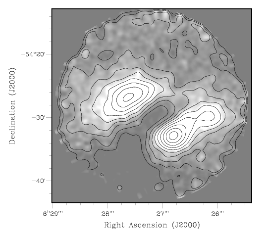
Figure 2: The exposure corrected combined image from MOS1 and MOS2 detectors after removing point sources and smoothing with a Gaussian kernel of width 17.5^′′. Overlaid contours are logarithmically distributed between $1.72\times 10^{-6}-8.78\times 10^{-6}$ counts s^-1arcsec^-2.

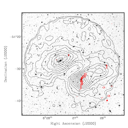
Figure 3: A3395 image from the SuperCOSMOS survey in the $B_{J}$ band with overlaid X-ray contours from Figure 2 (shown with black) and ATCA 1348 MHz radio continuum contours (shown with red; levels are at 0.005 times 1, 2, 4, 8, 16, and 32 Jy beam^-1).

The MOS1 and MOS2 images were combined together using the SAS tasks merge and evselect to increase the signal-to-noise ratio of the sources and reach fainter flux levels. Only those events that were spread over less than 4 pixels (i.e., pattern =0-12) were selected for producing the combined image. Point source extraction was done simultaneously on the MOS1, MOS2 combined image and the PN detector image using the SAS task edetect_chain which is a combination of several SAS tasks viz. eboxdetect (in local mode), esplinemap, eboxdetect (in map mode), and emldetect. When run in local mode eboxdetect produced source lists by collecting source counts in the cells of $5\times 5$ pixels and using a value of 8 for the minimum detection likelihood (eboxl_likemin) (i.e. a value of e^-8 for the minimum value of the probability of the Poissonian random fluctuation of the counts in the detection cell which would result in the observed number of source counts). Then esplinemap was used to generate background maps by using the source list generated by eboxdetect (in local mode) to remove point sources from the original merged image. Then eboxdetect (in map mode) uses these background maps to generate a new point source list (with fainter sources included). A total of 258 point sources were thus detected. Each of these detected sources was checked for each of the detectors and spurious sources (sources that did not look like actual sources in the individual detector images) were removed. Finally 77 sources for MOS1, 67 for MOS2, and 44 sources for PN were detected. Of these, 22 sources were found to be common in MOS1 and MOS2 and 13 were common in all three detectors. These detected sources were then removed from individual MOS1, MOS2 and PN images to create the cheesed images. The cheesed MOS1 and MOS2 images were combined using the procedure described in Snowden et al. (2008). A contour map of diffuse X-ray emission from A3395 using the combined MOS1 and MOS2 image after the removal of point sources and after applying the smoothing function is shown in Figure 2. Contours of the smoothed X-ray emission are also overlaid on the optical image of A3395 from the SuperCOSMOS survey in the $B_{J}$ band and shown in Figure 3. The optical image shows both the bright central galaxies (BCGs) for the NE and SW regions. The position of the BCG for the NE region coincides with the X-ray emission peak for the NE region whereas the BCG for the SW region is offset from the X-ray emission peak for the SW region by about $\sim 16.5^{\prime\prime}$ which is equivalent to $\sim 16$ kpc at the redshift of the cluster.

3.2 Chandra X-ray Observatory

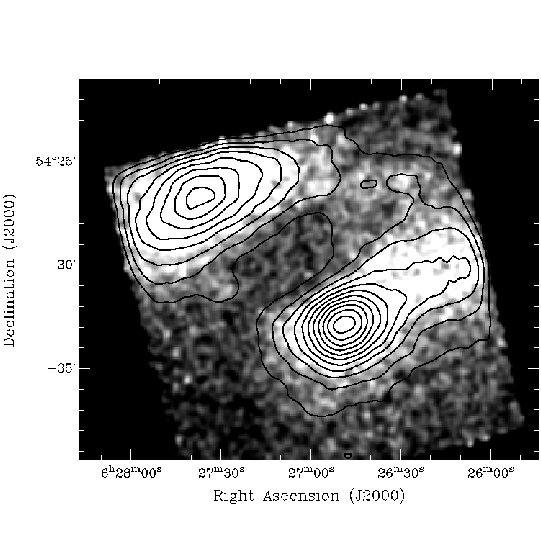
Figure 4: Exposure-corrected Chandra ACIS image of A3395 in the 0.3-7.0 keV band (after point source removal and smoothing with a Gaussian kernel of width 8^′′). The overlaid X-ray emission contours are at 2, 4, 6, 8, 10, 12 , 14, 16, 18, 20, 22, and 24 times $\sigma=1.16\times 10^{-8}$ counts cm^-2s^-1pixel^-1 level above the mean background level (=$4.67\times 10^{-8}$ counts cm^-2s^-1pixel^-1).

A3395 was observed with Chandra on 2004 July 11 (ObsID 4944) with ACIS-I detector for 22.2 ks (Table 1). The raw Chandra ACIS image is shown in Fig. 1. The data were analyzed with the CIAO version 4.3 and CALDB version 4.4.0. No reprocessing of data and time-dependent corrections were required as the ASCDSVER (keyword that stores the processing version information) is DS 7.6.7.2 and time-dependent corrections have become a part of standard data processing after DS 7.3.0. The standard Charge Transfer Inefficiency (CTI) corrections have been applied. Point sources were detected using the CIAO task wavdetect with the detection threshold fixed to the default value $10^{-6}$. A total of 47 bright sources were detected; 16 of these sources were common with the sources detected in the MOS 2 detector image, discussed in the previous section. The smoothed, point-source-removed and exposure-corrected Chandra image of the cluster in the 0.3-7.0 keV band is shown in Figure 4.

3.3 Australia Telescope Compact Array

A3395 was observed by A.D. Reid and R.W. Hunstead with ATCA on 1995 January 09. The pointing centre was 06^h 26^m 58.0^s, $-$54^d 31^′ 12.0^′′ (J2000) and centre frequencies were 1348 and 2374 MHz with bandwidths of 128 MHz. The array was in the 6A configuration, with baselines ranging from 337 to 5939 metres. The total integration time was 5.6 hours, consisting of multiple cuts spread over a wide range of hour angles. Primary flux density calibrator was B1934$-$638 and the phase calibrator was B0647$-$475.

Data reduction was carried out in MIRIAD (see Sault et al. 1995) using standard techniques. The restored beams were 11.0$\times$8.9 arcsec² along PA=$-$30.5^∘ at 1348 MHz, and 6.2$\times$5.0 arcsec² PA $-$32.5^∘ at 2374 MHz. The rms noise is 1.4 mJy beam^-1 in the 1348 MHz image and 1.3 mJy beam^-1 in the 2374 MHz image. A contour map of the 1348 MHz ATCA radio emission has been overlaid on the image from the SuperCOSMOS survey in the $B_{J}$ band and is shown in Fig. 3.

4 Analysis and Results

4.1 X-ray Morphology

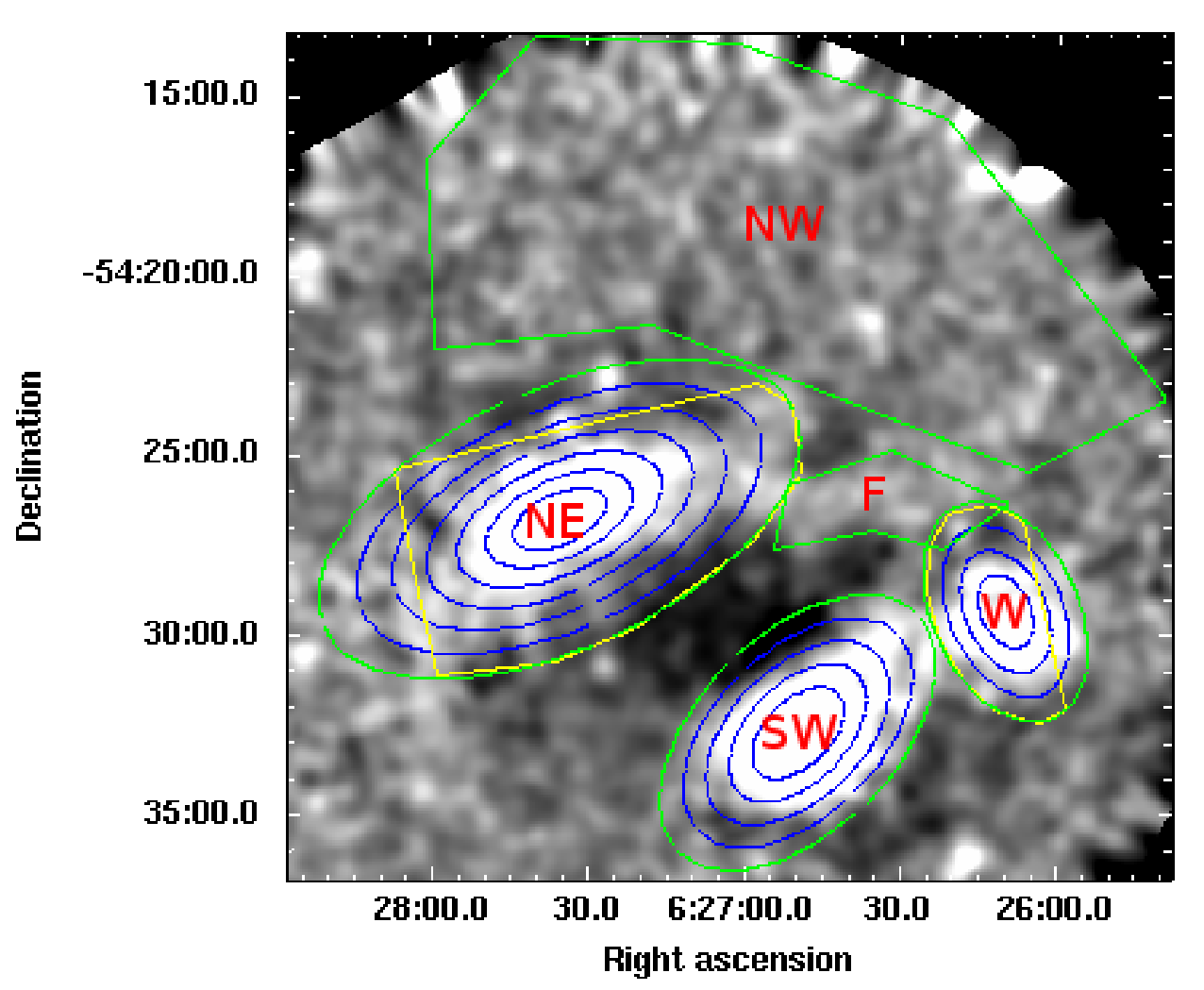
Figure 5: The unsharp-masked image of A3395 from the combined MOS1 and MOS2 detectors (produced by subtracting a large scale (100^′′) smoothed image from a small scale (15^′′) smoothed image) showing the four principal regions of emission : NE, SW, W, the filament connecting NE to W region (marked with an ’F’) and the NW region (reported by (Tittley & Henriksen, 2001)) used for extraction of spectra using XMM-Newton MOS1, MOS2 and PN detectors in section §4.3 with green. For extraction of spectra using Chandra data polygon shaped approximations (yellow) were made for the NE and W regions as Chandra did not cover these parts sufficiently, while regions used for the SW and filament regions were kept same. All the annuli regions, shown with green plus blue ellipses in all three subclusters were used in the azimuthally averaged spectral analysis using XMM-Newton and Chandra data in §4.4.1 and §4.4.2. Only the innermost 4 annuli in the NE and innermost 2 annuli in the W region were used for Chandra data.

Figure 5 shows the unsharp-masked image produced from the combined MOS1, MOS2 detector image, by subtracting a large scale (100^′′) smoothed image from a small scale (15^′′) smoothed image. Five distinct regions can be seen: the A3395 NE, A3395 SW, A3395 W, A3395 NW and a filament joining the NE region to the W region. The W region is a small and relatively faint subclump of diffuse emission visible towards the west of the SW region. Only two main X-ray peaks NE and SW, could be seen in the earlier X-ray images and are believed to be subclusters. Figs. 2 and 4 show a strong gradient in the surface-brightness in the southeast part of the SW component evident from the compression of X-ray contours in this part, indicating that the SW component is moving along the southeast direction. It appears that the small clump in the W region may also be a subcluster participating in the merger process. The Chandra image of the cluster (Fig. 4) does not fully cover the NE and W regions. None of the three regions in A3395 cluster show a circular symmetry. Therefore, for the analyses that follow, we have made elliptical approximations for them. The NE, SW, and W regions have been approximated as ellipses with semi-major-axis lengths 432.0^′′, 280.8^′′, and 194.4^′′, ellipticities 0.87, 0.81, and 0.78, and major-axis position angles $115^{\circ}$, $135^{\circ}$, and $25^{\circ}$ respectively, measured from the North in an anti-clockwise direction (shown with the green ellipses in Fig. 5). A3395 NW can be seen as a region of weak X-ray emission towards the north and northwest of the cluster in Fig.5. This excess emission was first reported by Tittley & Henriksen (2001). The optical image of A3395 NW shows a clustering of galaxies, however, its X-ray emission is very diffuse and does not seem to clump. The mean velocity of the group of galaxies associated with the NW, from the velocity data given in Teague, Carter, & Gray (1990) is $14540\pm 70$ km s^-1, while the same calculated from the velocity data given in Donnelly et al. (2001) is $15110\pm 130$ km s^-1. The data by Donnelly et al. put this group at almost the redshift of the NE and SW subclusters. Considering that A3395 NW lies along the filament joining the clusters A3395 and A3391 (Tittley & Henriksen 2001), it appears to be a part of the supercluster network.

4.2 X-ray Surface Brightness Profiles

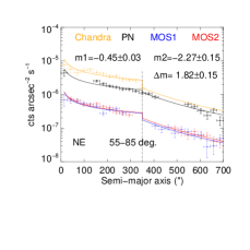
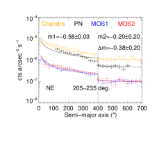
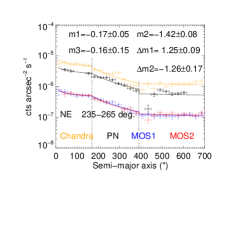
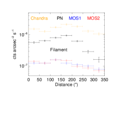
Figure 6: Surface brightness profiles from three sectors in the NE subcluster (Figures 6, 6 and 6) made by using MOS1 (Blue), MOS2 (Red), PN (Black) and Chandra ACIS (Orange) raw images after removing point sources, obtained from 25 elliptical annuli, each divided into 12 sectors. The profiles have been fitted with single or multiple powerlaws which are shown using solid lines and the positions of discontinuities are shown with dotted lines. The SW subcluster shows uniformly decreasing surface brightness profiles in all sectors (not shown here). The surface brightness profiles of the W region from the full $0^{\circ}-360^{\circ}$ range using 5 elliptical annuli and the filament from 8 rectangular regions approximately parallel to the length of the filament have been shown in Figures 6 and 6 respectively. Points affected by point source removal, individual CCD overlaps in a detector, and those lying within MOS1 CCD5 and MOS1 CCD6 have been removed. All angles are measured from the North and in the anti-clockwise direction.

Merging clusters like A3395 can host both shock and cold fronts which can be confirmed by surface-brightness and temperature discontinuities. The discontinuities are seen by a change in the slope of the profile. In order to search for these features, surface-brightness profiles for the NE, SW, and W regions were made. We have used the raw MOS1, MOS2, PN detector images (without any smoothing applied but with the point sources removed by applying the cheese masks generated by the $\textquoteleft$cheese$\textquoteright$ task) and the point-source-removed raw Chandra ACIS detector image to derive the surface-brightness profiles. We used 25 annuli in the NE, 10 annuli in the SW, and 9 annuli in the W regions centred at the intensity peaks in each of the NE, SW, and W regions, which were further divided into 12 sectors of $30\,^{\circ}$ each. The ellipses are such that the $n^{\rm th}$ ellipse for the NE region has a semi-major axis of $n\times 28.0^{\prime\prime}$, the SW region has a semi-major axis of $n\times 28.1^{\prime\prime}$, and the W region has a semi-major axis of $n\times 21.6^{\prime\prime}$. The major-axis position angles and ellipticities for the ellipses in NE, SW, and W regions were the same as given in section §4.1 and the $30^{\circ}$ sectors have been arranged symmetrically about the major-axes. To analyze the surface-brightness in the region between NE and SW subclusters, (which is not covered by the green ellipses in Fig. 5) and also to avoid overlaps between the three subclusters, the area spanned by the ellipses in the NE subcluster is larger, whereas that for the ellipses in the SW and W subclusters is almost same as compared to the green ellipses in Fig. 5. In the SW region, certain sectors had holes (due to point source removal) at the centre. Also, in the NE region, a few outermost annuli in the sectors with position angles from $55^{\circ}$ to $145^{\circ}$ had no MOS1 data (because of the missing CCD6 in MOS1), and with position angles from $295^{\circ}$ to $205^{\circ}$ had no Chandra data. In addition to this, the raw images had spurious discontinuities at the positions where the individual CCDs in a detector overlap. Points from all affected annular sectors were removed from the plots, but the resulting gaps made it more difficult to identify discontinuities. Surface-brightness profiles for all four detectors for each and every sector were obtained and were fitted by using single or multiple (for profiles showing more than one discontinuity) power laws. In order to make confident detections of discontinuities, we focused only on those discontinuities which are seen in all four detectors. All sectors in the NE and SW regions, in general, show a fairly uniform decreasing profile, except for a few sectors that show a change in the slope. The surface-brightness profiles of all sectors in the W region show a nearly constant profile. Only those surface-brightness profiles that show evidence for a significant change in slope are shown in Figure 6.

The $55^{\circ}$-$85^{\circ}$ sector (Figure 6) in the NE region shows a discontinuity at semi-major axis of $\sim 350^{\prime\prime}$. The sectors $205^{\circ}$-$235^{\circ}$ (Figure 6), and $235^{\circ}$-$265^{\circ}$ (Figure 6), in the NE region, show a flattening of the slope in all four detectors at a semi-major axis of $\sim 400^{\prime\prime}$. Starting from the centre of the NE component, this discontinuity is found at $\sim 3/4$ times the distance between the centres of the NE and SW regions ($d_{NE-SW}\sim 540^{\prime\prime}$). The observed flatness or increase in the surface-brightness in a region between the NE and SW subclusters is found to be due to the co-addition of the emission from the two subclusters. This result was confirmed by analyzing the sum of the $\beta$-models fitted to the surface brightness profiles of the $25^{\circ}-55^{\circ}$ sector in the NE (away from SW) and the $265^{\circ}-295^{\circ}$ sector in SW (away from NE), which showed a similar flatness in the same region between the NW and SW subclusters. A weak discontinuity in the sector $235^{\circ}$-$265^{\circ}$ is also seen at a semi-major axis of $\sim 170^{\prime\prime}$. All the sectors in the SW subcluster show a uniformly decreasing profiles. The surface-brightness profiles in all the sectors of A3395 W show a nearly constant profile. We also obtained the total surface brightness profiles of A3395 W over the full $0^{\circ}-360^{\circ}$ range by using 5 annuli centred at the emission peak of A3395 W and the filament by using 8 rectangular regions parallel to the length of the filament and placed almost symmetrically about it. The surface brightness profile of the W subcluster shows a decreasing profile from the innermost to the outermost annulus with a peak at the centre (Figure 6) while that of the filament shows a significant hump above the background at the centre (Figure 6).

4.3 Global X-ray Spectra

Average spectra of the various components of A3395 were extracted from both the XMM-Newton and Chandra data. For XMM-Newton, these spectra were extracted from elliptical regions for the NE, SW and W components, and from polygon shaped regions for the NW component and the filament. The ellipses were centred on the peaks of the surface-brightness. The ellipse for the NE region had a semi-major axis of 432^′′ and an ellipticity of 0.87, the SW region had a semi-major axis of 281^′′ and an ellipticity of 0.81, and the W region had a semi-major axis of 194^′′ and an ellipticity of 0.78. For the spectral extraction using Chandra data, the regions used for the SW and the filament were the same as those used for XMM-Newton, while for the NE and W, maximum possible areas were picked by using a polygon shaped region, since Chandra field does not cover these regions fully. As the NW region was not covered by Chandra, its spectral analysis was done using only XMM-Newton detectors. All these regions are shown in Figure 5. All spectra were extracted in the energy band 0.5-9.0 keV. For MOS data, events with $\rm PATTERN\leq 12$ were used, whereas for PN data, events with $\rm PATTERN\leq 4$ were selected. For XMM-Newton detectors, the response matrices and effective areas were generated using the tasks rmfgen and arfgen. The neutral hydrogen column density along the line of sight to the cluster (i.e., along $\alpha=06^{\rm h}27^{\rm m}31.1^{\rm s}$, $\delta=-54^{\rm d}23^{\prime}58^{\prime\prime}$) was taken to be $6.3\times 10^{20}$ cm^-2 based on Leiden/Argentine/Bonn (LAB) Galactic HI survey (Kalberla et al. 2005) and redshift was frozen to the value of 0.0498 (SIMBAD astronomical database).

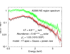
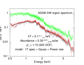
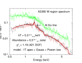
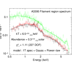
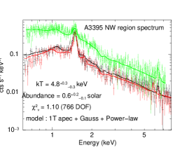
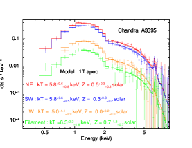
Figure 7: Figure 7 to 7: Average spectra of the A3395 NE, SW, W subclusters, the filament connecting NE to W, and the NW region (reported by (Tittley & Henriksen, 2001)), produced by using the XMM-Newton PN (Green), MOS1 (Black), and MOS2 (Red). Figure 7 : Average spectra of NE, SW, W subclusters and the filament produced using Chandra data. All the spectra have been fitted with wabs*apec model shown as a histogram. The powerlaw and Gaussian components in the XMM-Newton spectra have been added to model the residual soft proton contamination and the instrumental Al line at 1.49 keV. Details of spectral analysis are given in §4.3, and the best fit parameters are shown here as insets.

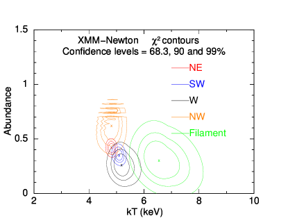
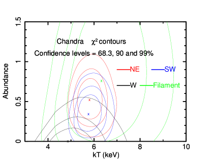
Figure 8: 8 : $\chi^{2}$ contours of the temperature and abundance measurements for the NE (red), SW (blue), W (black) and NW (orange) regions of A3395 and the filament connecting NE to W (green) from the spectral analysis done using XMM-Newton data. 8 : $\chi^{2}$ contours of the temperature and abundance measurements for the NE (red), SW (blue) and W (black) regions and the filament (green) from the spectral analysis done using Chandra data. Details of the spectral analyses are given in §4.3. The confidence levels for the innermost, middle, and outermost contours for each of the 9 sets of contours are at 68.3%, 90% and 99% respectively.

Spectral analyses have been performed using the X-ray spectral fitting package Xspec (version 12.5.1). Spectra extracted from all detectors were fitted using the wabs photoelectric absorption model (Morrison & McCammon 1983) and apec plasma emission model (Smith et al. 2001). The relative elemental abundances used in wabs are as given by Anders & Ebihara (1982). The MOS1, MOS2 and PN spectra for each of the regions were fitted simultaneously using three separate wabs*apec models. The values of abundance, temperature and apec normalizations for the models were linked together but were not frozen. The MOS1, MOS2 and PN spectra of the weak emission regions viz. the NW, the W and the filament showed presence of residual soft proton contamination (shown by prominent residues in the high energy end of the spectra) and the residual instrumental Al K-$\alpha$ line at 1.49 keV. The residual soft proton contamination was modeled by using separate powerlaw models with diagonal RMF files (Snowden et al. 2008) and the instrumental Al K-$\alpha$ line at 1.49 keV was modeled by adding Gaussian components separately for MOS1, MOS2 and PN (Snowden et al. 2008). The powerlaw indices were found to be negative for most cases and hence were frozen to the value of 0.3 (i.e. the minimum recommended in Snowden et al. 2008), while the powerlaw normalizations were left as free parameters. The centre position and the widths of the Gaussian components were frozen to 1.49 keV and 0.02 keV respectively in all the spectra and their normalizations were left as free parameters. The resulting spectra, along with the histograms of best fit model spectra are shown in Figure 7 and the best fit values of the temperature, abundance and apec normalizations from the XMM-Newton and Chandra spectral analyses are given in Tables 2 and  3 respectively. The confidence contours at the 68.3%, 90% and 99% confidence levels for the free parameters are shown in Figure 8.

From the confidence contours produced from the spectral analysis using XMM-Newton, it can be seen that the values of the temperatures and abundances for the NE and the SW regions; the NE and W regions and the NW and W regions are different only at a confidence level of 68.3%. However, the temperature and abundance values for the SW and W regions hardly differ. The temperature and abundance values for the filament appear to be distinct from the values for all other components except for the W region, which are distinct only at a confidence level of 68.3%. The best fit parameters from Chandra have errors much larger than those from XMM-Newton because of fewer counts and hence, all four sets of confidence contours have large overlaps. While the results for all other regions are in agreement with those from XMM-Newton (within errors), the results from Chandra for the NE region show a temperature slightly higher than that from XMM-Newton. This is possibly because the part of NE which is not covered by Chandra has a lower than average temperature, as is indicated by the temperature map produced from XMM-Newton data in §4.5. This was also confirmed by using the same polygon shaped region for the extraction of spectrum from the NE with MOS1, MOS2 and PN, as was used for Chandra spectral analysis, and the results were in mutual agreement. The background systematic errors (assuming 10%) do not affect the results significantly.

4.4 Azimuthally Averaged spectrally determined radial profiles of thermodynamic quantities

We also produced azimuthally averaged profiles of temperature, density, entropy, and pressure for the cluster by extracting spectra in elliptical annuli using both XMM-Newton and Chandra data. The NE, SW, and W subclusters were divided into 7, 5 and 4 elliptical annuli respectively (shown in Figure 5). The centres of the ellipses were at the peak of the X-ray emission for all three regions. Ellipses in the NE regions had semi-major axis lengths of 84^′′, 132^′′, 184^′′, 240^′′, 300^′′, 364^′′, and 432^′′. Similarly, ellipses in the SW region had semi-major axis lengths of 93.6^′′, 140.4^′′, 187.2^′′, 234^′′, and 280.8^′′ and W region had semi-major axis lengths of 64.8^′′, 108^′′, 151.2^′′, and 194.4^′′. Spectra were extracted from all the annuli for all three detectors of XMM-Newton. However, for Chandra data, only the innermost 4 annuli in the NE and innermost two annuli in the W region were used as Chandra did not cover the NE and W parts completely, while for the SW subcluster, spectra were extracted from all 5 annuli. All the spectra were extracted in the energy band of 0.5-9.0 keV. Both the projected and deprojected profiles of temperature, density, entropy, and pressure were obtained.

4.4.1 2-D Projected Profiles

The details of spectral analyses performed are the same as given in §4.3 except that the elemental abundances were fixed to the respective average abundance value obtained from the spectral fitting of the NE, SW, and W regions using XMM-Newton data i.e., 0.42, 0.35, and 0.3 times the solar value ($Z_{\odot}$) (Table 2.) respectively, for the annuli belonging to the respective region. The temperature profile was obtained directly from the spectral analysis and was used to derive the density, entropy, and pressure profiles. To derive the electron density n_e, we used the apec normalization, K$=$10^-14EI/(4$\pi$[D_A(1+z)]²) (expressed in units of cm^-5 in cgs system), where EI is the emission integral $\int\rm n_{\rm e}\rm n_{\rm p}$dV. We assume $\rm n_{\rm p}=0.855\rm n_{\rm e}$ (Henry et al. 2004), which under the assumption of constant density within each ellipsoidal shell gives, EI$=0.855\rm n_{\rm e}^{2}$V, where V$=$volume of ellipsoidal shell. For the volume estimation of the ellipsoidal shells we have assumed oblate ellipsoids (i.e., line of sight axis = major-axis of the ellipse). Then the volume of a shell, V$=(4\pi/3)(\rm a_{\rm out}^{2}\rm b_{\rm out}-\rm a_{\rm in}^{2}\rm b_{\rm in})$, where $\rm a_{\rm out}$ and $\rm b_{\rm out}$ are the semi-major and semi-minor axis of the outer shell and $\rm a_{\rm in}$ and $\rm b_{\rm in}$ are those of the inner shell. From the commonly adopted definition, entropy is given by S$=\rm kTn_{\rm e}^{-2/3}$ and electron pressure P$=\rm n_{\rm e}\rm kT$ (Gitti et al. 2010). If the ions have the same temperature as that of the electrons then the total pressure is twice as large. We admit that the volume estimates may introduce errors $\sim 20\%$ (Finoguenov et al. 2004, and references therein; Henry et al. 2004), but even these errors are quite small as compared to the errors in temperatures obtained from the deprojection analysis because of poor statistics of the data. For confirmation we also estimated the entropy and pressure for prolate ellipsoidal shells (i.e., line of sight axis = minor-axis of the ellipse) but the differences were very small ($\sim 20\%$).

4.4.2 Deprojected Profiles

Projection effects along the line of sight can smooth out the variations in the measured quantities. To correct for this we have performed the deprojection analysis on the same annular regions shown in Fig. 5 by using the Xspec projct model, which estimates the parameters in 3-D space from the 2-D projected spectra of ellipsoidal shells, using the wabs*apec model. The model calculates the geometrical weighting factor according to which the emission is redistributed amongst the projected annuli. The elemental abundances for the annuli belonging to the NE, SW, and W regions were fixed to 0.42, 0.35, and 0.3 times the solar value ($Z_{\odot}$), same as in §4.4.1. The residual soft proton contamination and instrumental Al lines were modeled by adding powerlaws and Gaussian components to the models as described in §4.3 with the only difference that a single model for all MOS1, MOS2 and PN was used. This was because the projct model requires all the spectra belonging to the same annulus to be part of the same group and therefore have to be modeled using the same model. Electron density n_e, entropy (S), and electron pressure (P) have been calculated using the same relations as given in §4.4.1.

The resulting projected and deprojected temperature and density profiles are shown in Figure 9, and the projected and deprojected entropy and pressure profiles are shown in Figure 10. Best fit parameters and the derived values of other dependent parameters are given in Tables 4- 7. The projected spectral analysis resulted in a nearly constant temperature profile for all three subclusters, while the projected density, entropy, and pressure profiles show a uniform decrease, increase, and decrease respectively for all three subclusters from the innermost to the outermost annulus. The deprojected temperatures, entropies and pressures of all the three subclusters show a nearly uniform profile. The deprojected density profiles from all three regions show a uniform decrease except for the outermost annulus where a slight increase in the density is seen. This is a common artifact of deprojection analysis because the excess emission from shells with radii larger than that of the outermost annulus, gets added to the outermost annulus. The projected profiles from Chandra and XMM-Newton are in complete agreement with each other although the former has larger errors as compared to the latter. For the deprojected profiles also, there is a good agreement in the results between XMM-Newton and Chandra with a few anomalies. For example, the deprojected density for the innermost annulus in the NE region from Chandra is greater while the density in the second annulus in the W region from Chandra is lower as compared to those from XMM-Newton. However, the higher deprojected density and pressure from Chandra in the fourth annulus (outermost annulus for Chandra) in NE as compared to those from XMM-Newton can easily be explained as the artifact of deprojection described earlier in this section.

4.5 Spectrally determined 2-D projected thermodynamic maps at a higher resolution

We have made projected temperature, abundance, density, entropy, and pressure maps of A3395, using box shaped regions for spectral analysis to improve the spatial resolution of the spectral parameters and to look for anisotropy in their spatial distribution. To make the results more robust, both XMM-Newton and Chandra data have been used and the whole cluster was divided into 139 boxes for XMM-Newton and only 42 boxes for Chandra. The number of boxes used for Chandra were less because of fewer counts and also because Chandra did not cover the outer parts of the cluster significantly due to smaller FOV. The sizes for the boxes were chosen adaptively to get sufficient counts in each region. For XMM-Newton, large size boxes ($\sim 3.1^{\prime}\times 1.4^{\prime}$ or $\sim 1.6^{\prime}\times 2.9^{\prime}$) for the outermost parts, small size boxes ($\sim 47^{\prime\prime}\times 43^{\prime\prime}$) for the innermost brightest parts, and medium sized boxes ($\sim 1.6^{\prime}\times 1.4^{\prime}$) for the regions in between were made to get more than 700 total counts from all three detectors in each box. For Chandra, large size boxes ($\sim 3.1^{\prime}\times 1.6^{\prime}$) for outer parts and small size boxes ($\sim 1.6^{\prime}\times 1.6^{\prime}$) for the inner parts were made to get more than 700 counts in each box. Hence, spatial resolution of the thermodynamic maps obtained with XMM-Newton is better than that from Chandra. Spectra from all boxes were fitted using wabs*apec model with fixed Galactic absorption. The residual soft proton contamination and instrumental Al lines were modeled by adding powerlaws and Gaussian components to the models as described in §4.3. For the boxes where MOS1 data could not be used (i.e., boxes lying in regions of MOS1 missing CCD6 and anomalous CCD5), only MOS2 and PN spectra were used. The electron density, entropy, and electron pressure were calculated using the same relations as in §4.4.1. The volume calculation for the box regions, however, was not as straightforward as in the case of ellipsoidal shells. We had to assume spherical geometry which can be justified because the volumes considered here are very small as compared to those for the ellipsoidal shells. We assumed the 139 box regions as projections of parts of spherical shells (centred at the X-ray intensity peak of the subcluster nearest to the box) with inner and outer radii (R_in, R_out) equal to the smallest and largest distance from the centre of their respective spheres. The volume for each box region was estimated as D${}_{\rm A}^{3}\rm\Omega(\rm\theta_{\rm out}^{2}-\rm\theta_{\rm in}^{2})^{1/2}$ (Ehlert et al. 2010; Henry et al. 2004), where $D_{A}$ is the angular diameter distance and $\rm\Omega$ is the solid angle subtended by the region. $\rm\theta_{\rm in}$ and $\rm\theta_{\rm out}$ are equal to the distances R_in and R_out expressed in angular units respectively.

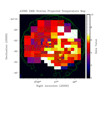
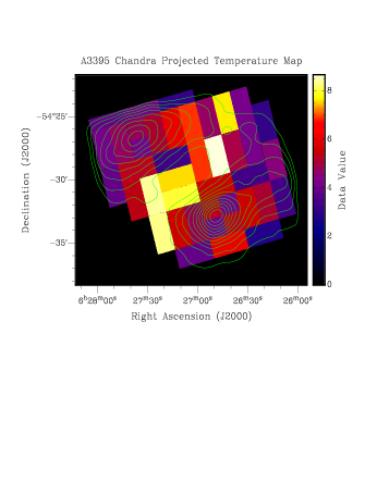
Figure 11: Projected temperature maps from 139 box regions using XMM-Newton data (top) and 42 box regions using Chandra data (bottom) with overlaid X-ray surface-brightness contours having levels same as in Figs. 2 and 4 respectively. The scales are expressed in keV units shown in the bars alongside. Details of the spectral fittings are provided in §4.5.

The temperature, density, entropy, and pressure maps produced (from both XMM-Newton and Chandra) are shown in Figures 11,  12,  13, and  14 respectively. Maps obtained from Chandra had larger errors as compared to those from XMM-Newton, and in all the maps fainter regions had larger errors. The errors range from as low as $\sim$15% for the innermost regions of NE and SW subclusters to as high as $\sim$60% for the extreme outermost box regions and the highest temperature regions in the NW and towards the southeastern edge of the SW. Abundance values had large errors in the maps obtained from both XMM-Newton and Chandra and for most of the boxes only upper limit of abundance could be obtained, hence the abundance maps have not been shown. Maps from both XMM-Newton and Chandra show a high temperature and high entropy region where the NE and SW regions meet. The SW, on an average shows a temperature slightly higher than the average temperature of the NE and even more higher temperature regions are seen in the W component, the region joining the NE and SW parts and the filament regions. The NE and SW components have similar average entropies and the W component has slightly higher average entropy. The filament and the region between the NE and SW components have even higher entropies. The highest temperatures and entropies are seen at the south-eastern edge of the SW subcluster and in a few regions in the NW component lying above the filament, to the west of the NE subcluster. Although, the single apec model provided a good fit for the source spectra of all the regions, for some of the regions (for e.g., the region between the NE and SW) they could also be very well fitted using powerlaw model (in addition to the fixed index powerlaws used for modeling the residual soft proton contamination), thus pointing towards a completely non-thermal emission from shock accelerated particles. None of the two models seemed to be statistically preferred. Fitting the spectra with apec+power-law or two apec models resulted in the values of the free parameters being insensitive to the fits. In addition, the normalizations of the non-thermal (power-law) components in the apec+power-law fits were found to be negligible as compared to those of the thermal (apec) components.

4.6 Radio sources

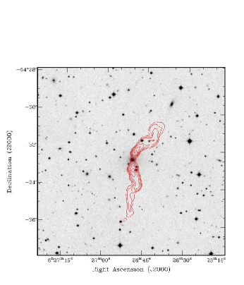
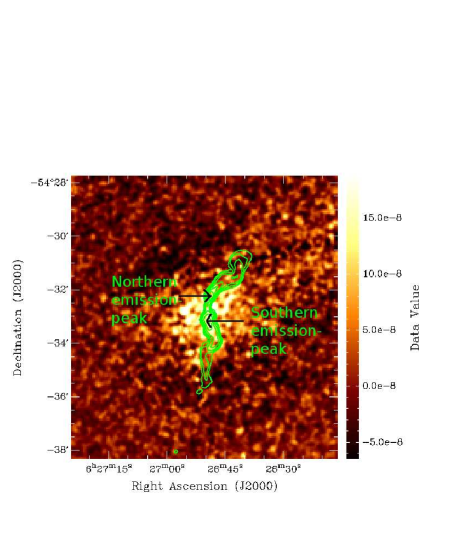
Figure 15: 15 : Optical image from the SuperCOSMOS survey in the $B_{J}$ band of the region surrounding the WAT source in A3395 SW overlaid by ATCA 1348 MHz radio continuum contours. Contour levels are at 0.005 times 1, 2, 4, 8, 16, and 32 Jy beam^-1. 15 : Chandra unsharp-masked image produced by subtracting a large scale (80^′′) smoothed image from a small scale (4^′′) smoothed image of the same region as 15 overlaid by the same ATCA 1348 MHz radio continuum contours (green). Positions of the northern and southern emission peaks have also been shown. The colour scale shown as a bar is expressed in units of counts s^-1arcsec^-2.

The ATCA images at 1348 and 2374 MHz show that the most prominent source in the field is the wide-angle tailed (WAT) source PKS B0625$-$545 (MRC B0625$-$545) which is identified with an elliptical galaxy at a redshift of 0.05174 (Teague, Carter, & Gray 1990) (Figure 15). Both the oppositely-directed jets bend initially towards the west and then again bend sharply further down the flow at $\sim$90 kpc from the host galaxy so that the emission is approximately along the north-south axis. Douglass et al. (2008) have observed similar bends in the WAT source in Abell 562 and have interpreted the bends further down the flow as the regions where the effects of buoyancy become important. Figure 15 shows the unsharp-masked Chandra image of the cluster (zoomed in to show the WAT source) produced by subtracting a large scale (80^′′) smoothed image from a small scale (4^′′) smoothed image, overlaid with the 1348 MHz radio continuum contours. It may be worth noting that there is no evidence of X-ray cavities associated with the regions of radio emission.

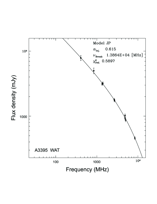
Figure 16: The radio spectrum of the complete WAT source in A3395 SW, as described in the text. The flux density measurements have been fitted for the (Jaffe & Perola, 1973) model using the SYNAGE package ((Murgia et al., 1999)).

The flux densities of the WAT galaxy at a number of frequencies from low-resolution observations are listed in Table 8, including the values listed by Burgess & Hunstead (2006), and estimates from the ATCA images presented in this paper. The flux density estimated from the ATCA image at 1348 MHz is very close to the measurement at 1410 MHz, suggesting that the interferometric observations at this frequency have not missed any significant amount of flux density. However the expected flux density at 2374 MHz from the derived spectrum using the high-frequency points ($>$800 MHz) is higher than our measured value by $\sim 20\%$. Although the high-frequency points are consistent with a straight spectrum with a spectral index of $\sim$1.05, a good fit to the spectrum is obtained for the Jaffe & Perola (1973) model using the SYNAGE package (Murgia et al. 1999). Excluding the ATCA estimate at 2374 MHz where some flux density is missing, the spectrum is well fitted with an injection spectral index of 0.62 and a break frequency of $\sim$13.9 GHz (Figure 16). Higher frequency observations would be useful to determine this more reliably.

Besides the WAT galaxy, there is a head-tail (HT) source located at RA(J2000): $06^{\rm h}25^{\rm m}56.7^{\rm s}$ and Dec.(J2000): $-54^{\rm d}27^{\prime}50^{\prime\prime}$ which is associated with a galaxy at a redshift of 0.05955 (Teague, Carter, & Gray 1990) and is shown in Figure 3. The extent of the HT galaxy is smaller than the WAT, with an angular size of $\sim 80^{\prime\prime}$ including the diffuse emission, which corresponds to a linear size of $\sim$90 kpc at the redshift of the galaxy. The peak and total flux densities of the HT source at 1348 MHz are 25 mJy beam^-1 and $\sim$150 mJy. The tail is not as well imaged at 2374 MHz where the peak and total flux densities are 8 mJy beam^-1 and $\sim$70 mJy respectively. MOST observations show that the peak and total flux densities of the HT source are 135 mJy beam^-1 and 299 mJy respectively at 843 MHz (Reid 2000). The HT galaxy is located at the periphery of the W region of A3395. HT galaxies are often detected in non-relaxed cluster but can also be found in the periphery of clusters and near regions of enhanced X-ray emission (cf. Klamer, Subrahmanyan & Hunstead 2004; Mao et al. 2009, and references therein).

In addition, Reid (2000) lists two radio sources towards the NE region, namely J0627$-$5425 (RA (J2000): $06^{\rm h}27^{\rm m}18.8^{\rm s}$, Dec.(J2000): $-54^{\rm d}25^{\prime}10^{\prime\prime}$) identified with a dumbbell system at a redshift of 0.04512 (Teague, Carter & Gray 1990), and J0627$-$5426 (RA (J2000): $06^{\rm h}27^{\rm m}44.9^{\rm s}$ and Dec (J2000): $-54^{\rm d}26^{\prime}46^{\prime\prime}$), associated with a galaxy at a redshift of 0.04348. Both sources have been shown in Figure 3. The peak and total flux densities estimated from the ATCA image at 1348 MHz are 14 mJy beam^-1 and 46 mJy respectively for J0627$-$5425. The corresponding values for J0627$-$5426 are 6.9 mJy beam^-1 and 17 mJy respectively. The redshifts of these sources are much below the average redshifts (z=$\overline{\rm v}/c$) of the main components of A3395, hence these sources are most probably not cluster members.

4.7 X-ray Luminosity estimates

X-ray luminosities for the NE, SW, W, NW and the filament regions using XMM-Newton and for the NE, SW, and W and the filament regions using Chandra in the energy range 0.5-9.0 keV were estimated from the flux values obtained from the spectral analysis of these regions described in §4.3. The fluxes ($\rm F_{\rm X}$) were estimated by convolving the model used in §4.3 with the Xspec convolution model, cflux after freezing the apec normalization. The X-ray luminosities ($\rm L_{\rm X}$) were then obtained from the fluxes using the formula:

$$\rm L_{\rm X}=4\pi\rm D_{\rm L}^{2}\rm F_{\rm X}$$ (1)

where $\rm D_{\rm L}$ is the luminosity distance to the source. The luminosities (L_x), derived from the flux values obtained from the spectral analysis done using XMM-Newton and Chandra data are given in Tables 2 and  3 respectively. We also obtained the bolometric luminosities of the NE, SW, W and NW components. For this purpose, we fitted the $0^{\circ}-360^{\circ}$ surface brightness profiles of the NE, SW and W subclusters using $\beta$-profiles and the average count rates were obtained from the same regions as in §4.3. For the NW component the average count rate was obtained from an elliptical region (an approximation to the polygon shaped region used for the NW in section §4.3) with semi-major and semi-minor axis lengths of $11.11^{\prime}$ and $4.45^{\prime}$ respectively. By using the HEASARC tool Web Portable, Interactive, Multi-Mission Simulator (WebPIMMS), these count rates were converted to fluxes in the energy range of 0.01-100 keV from which bolometric X-ray luminosities were obtained using the relation given above in this section. The results obtained from the $\beta$-model fitting along with the estimated X-ray bolometric luminosities of the NE, SW, W and NW components have been given in Table 9. Xue and Wu (2000) obtained the L_X-kT relations based on 274 clusters and 66 groups as $\rm L_{X}=10^{-0.032\pm 0.065}T^{2.79\pm 0.08}$ and $\rm L_{X}=10^{-0.27\pm 0.05}T^{5.57\pm 1.79}$ for clusters and groups of galaxies respectively, where L_X is in units of 10⁴³ ergs s^-1 and T is in units of keV. On comparing the bolometric X-ray luminosities and temperatures of the NE, SW, W and NW components of A3395 with those obtained from these relations, we find that the NE, SW and W subclusters have bolometric X-ray luminosities within a factor of 1.5-2 of each other, and are close to the L_X-kT relation for the rich clusters obtained by Xue and Wu (2000). The temperatures of these regions are almost twice those of the rich clusters of similar luminosities. However, the NW component is sub-luminous by about an order of magnitude, as compared to the rich clusters of similar temperatures and is hotter as compared to the isolated groups of similar luminosities. From these observations, it seems highly probable that all the components of the cluster have been heated up due to the ongoing merger processes.

4.8 Gas Mass

The projected gas densities obtained from §4.4.1 for different annuli in the NE, SW, and W regions were fitted using a $\beta$-model i.e.,

$$\rm n_{\rm e}(\rm r)=\rm n_{\rm e}\left(0\right)\left(1+\frac{\rm r^{2}}{\rm r_{\rm c}^{2}}\right)^{(3/2)\rm\beta},$$ (2)

where $\rm n_{\rm e}(0)$ is the central density and $\rm r_{\rm c}$ is the core radius. The gas mass $\rm M_{\rm gas}(r)$ out to radii 0.5 Mpc and 1 Mpc for the NE, SW, and W regions were obtained by using the following formula (see Donnelly et al. 2001) :

$$\rm M_{\rm gas}(\rm r)=4\pi\rho_{0}\int_{0}^{\rm r}\rm s^{2}\left[1+\left(\frac{\rm s}{\rm r_{\rm c}}\right)^{2}\right]^{(3/2)\rm\beta}ds$$ (3)

where $\rho_{0}=\rm\mu\rm n_{\rm e}(0)\rm m_{\rm p}$ ; $\rm m_{\rm p}$ is the mass of a proton, and $\mu$= 0.609 is the average molecular weight for a fully ionized gas (Gu et al. 2010). The values of $\rm\beta$, $\rm r_{\rm c}$, $\rm\rho_{0}$, and $\rm M_{\rm gas}$ based on fitting the density profiles with the above model are listed in Table 10. The deprojected densities have not been used for determining the gas masses as they had very poor $\beta$-model fits, even after ignoring the outermost annuli densities, which were mostly an overestimate. The results, therefore, had large errors, especially for the W subcluster. A rough estimate for the gas mass of the NW component was also made by assuming a constant density in an oblate ellipsoid made from the ellipse used for the NW region in §4.7. The density was derived from the apec normalization obtained from the spectral analysis of NW region in §4.3 using the relation given in §4.4.1 and the gas mass was estimated to be $\sim(1.1\pm 0.2)\times 10^{12}$ M_⊙.

4.9 Cooling time

Using the central gas temperatures ($\rm T_{\rm g}$) and densities (n) derived from the deprojection analysis in §4.4.2 using XMM-Newton data and by using the equations from Sarazin (1988), we calculate the cooling times for the three regions NE, SW, and W of A3395, assuming them to be subclusters, as :

$$\rm t_{\rm cool}=8.5\times 10^{10}\rm yr\left[\frac{\rm n}{10^{-3}\rm cm^{-3}}\right]^{-1}\left[\frac{\rm T_{\rm g}}{10^{8}K}\right]^{1/2}$$ (4)

The cooling times for the NE, SW, and W subclusters are $2.9\times 10^{10}$y, $2.7\times 10^{10}$y, and $4.3\times 10^{10}$y respectively, which are much longer than the Hubble time. This shows that none of the subclusters has any ongoing cooling flow in it.

5 Discussion

The present X-ray observations of A3395 show that the cluster morphology is much more complex than the simple bimodal structure reported earlier. We identify four distinct regions of strong diffuse X-ray emission, namely, the NE, SW, W, and the filament connecting the W to the NE part of the cluster. In addition, a fifth component A3395 NW is seen as a weak excess emission in the northwest of the cluster, which was also detected by Tittley & Henriksen (2001) and is most probably a part of the supercluster filament connecting the clusters A3395 and A3391. Because of a larger FOV, better sensitivity, and larger energy band coverage of the XMM-Newton, we have been able to better constrain the values of the X-ray temperature and luminosities for the NE and SW subclusters, as compared to their values from earlier observations that used ROSAT and ASCA data. The temperatures determined by us for the NE ($4.8\pm 0.1$ keV) and SW ($5.1\pm 0.1$ keV) subclusters are very close (within uncertainties) to the values reported earlier by Markevitch et al. (1998) ($\sim$5.8$\pm$0.8 keV for the NE and $\sim 5.5\pm 0.8$ keV for the SW subcluster) based on ASCA data. We have estimated the X-ray luminosities of all the components of the cluster in the energy range of 0.5-9.0 keV and the values are given in Tables 2 and 3. A3395 NE is clearly the dominant subcluster with the highest X-ray luminosity and extent of emission. Our estimates of the bolometric X-ray luminosity for the NE subcluster is equal to, while that for the SW subcluster is slightly higher than, those from Donnelly et al. (2001), who estimated the bolometric X-ray luminosity within 1 Mpc of the NE and SW subcluster cores based on the surface brightness profiles using ROSAT data. In addition to the previously identified SW subcluster, there are strong indications for a separate clump W in the west that is either a clump of gas stripped-off the SW subcluster or is probably a separate subcluster merging with the A3395 SW. This W region is particularly delineated in the unsharp-masked MOS2 image shown in Fig. 5. Note that, in contrast to Donnelly et al. (2001), our estimate of the luminosity for the SW subcluster does not include the W region.

We now examine whether the W clump of X-ray emission represents a smaller group of galaxies in the process of merging in A3395.

5.1 Subclustering Analysis

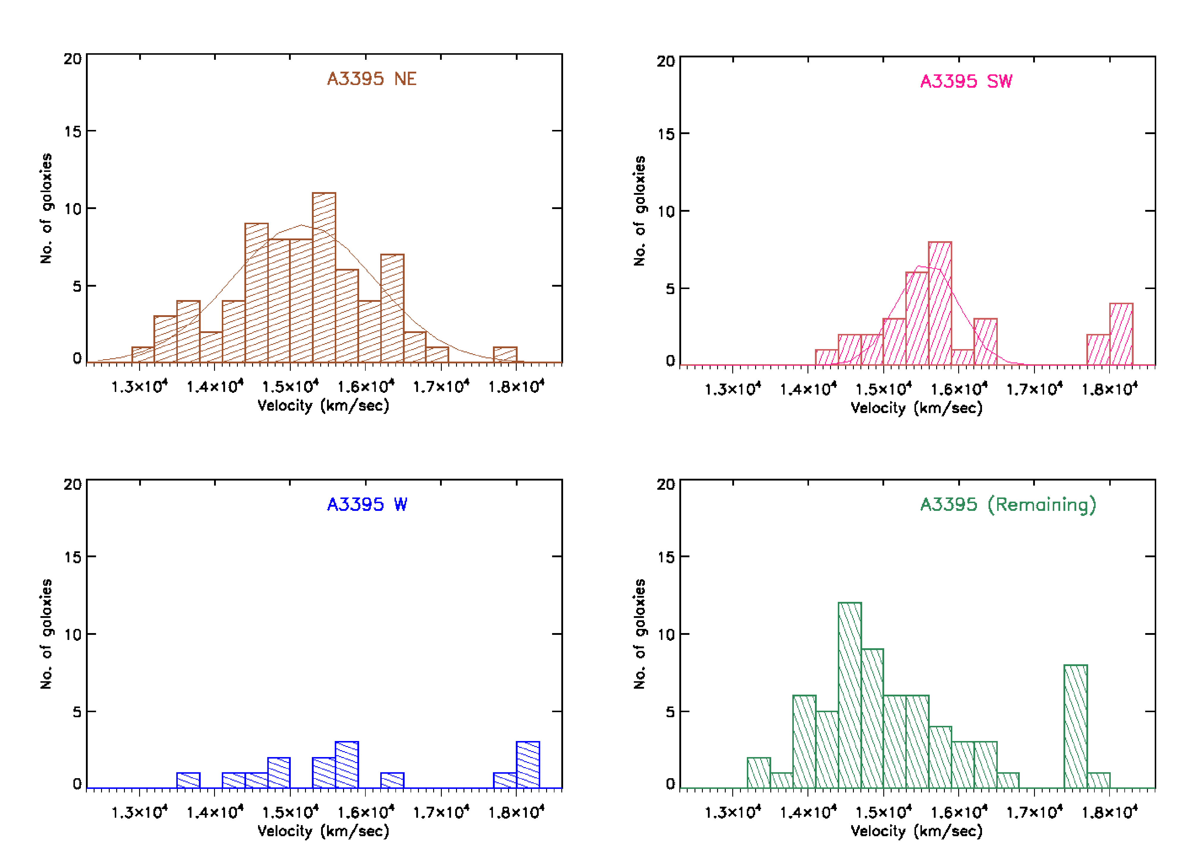
Figure 17: Velocity histograms of the galaxies belonging to the NE, SW, W subclusters, and the remaining set of galaxies that did not belong to any of the subclusters. Bins are 300 km s^-1 wide. Overlaid are the Gaussian fits to the velocity distribution of the NE and SW subclusters.

A3395 W appears to be a distinct region of X-ray emission (Figs. 2 to 5). The detection of an HT source at the periphery of the W subcluster, which is indicative of enhanced X-ray emission and a deep potential well, points towards a distinct atmosphere of the W subcluster. The surface brightness profile of the W subcluster (Fig. 6) which shows a peak at the centre, also strengthens the idea of a distinct identity of the W subcluster. We have also re-examined the galaxy velocity sample for A3395 from Donnelly et al. 2001, which had velocity information for 157 cluster member galaxies to look for dynamical evidence for A3395 W being a separate group. We divided the galaxies into the three subclusters by considering ellipses with major axes 0.4, 0.3, and 0.2 times $R_{180}$ (=34.6^′) for the NE, SW, and W subclusters respectively and counting the number of galaxies in these regions. The major-axis position angles and ellipticities for the ellipses in NE, SW, and W regions were the same as given in section §4.1. This led to 71 galaxies in the NE, 32 galaxies in the SW, and 15 galaxies in the W subcluster, leaving 69 galaxies which could not be clearly identified as belonging to any particular subcluster. Also, there were some slight overlaps in the three sets of galaxies. For example, NE and SW subclusters had 13 galaxies in common ; NE and W subclusters had 9 galaxies in common, and SW and W subclusters had 12 galaxies in common. The velocity histograms obtained for the four sets are shown in Figure 17, where the bin-size was chosen to be 300 km $\mathrm{s}^{-1}$ wide. Donnelly et al. (2001) had reported a high velocity hump in A3395. From Fig. 17, we observe that the galaxies in this hump belong to either the SW or the W parts or to none of the subclusters. The average subcluster velocities and their dispersions were obtained by fitting Gaussians to their velocity distributions and are given in Table 11. The velocity data in the W region shows a very flat and wide distribution and is not sufficient for fitting a Gaussian. In addition, the galaxies in the W subcluster seem to follow the velocity distribution of the SW subcluster.

Though the velocity distribution of the W subcluster had a very poorly fitted Gaussian, we have force-fitted a Gaussian to it for getting an estimate for the velocity dispersion and a lower limit of the virial mass used in the bound system analysis in §5.1.1. We estimated the virial mass for each of the subclusters assuming that the galaxies included in each subcluster are bound and the velocity dispersions are isotropic. We used the following formula (see Beers, Geller, & Huchra (1982)):

$$\rm M_{\rm virial}=\frac{3\pi}{\rm G}\sigma_{\rm r}^{2}\left\langle\frac{1}{\rm r_{\rm p}}\right\rangle^{-1}$$ (5)

where $\sigma_{\rm r}$ is the velocity dispersion along the line of sight and $\langle 1/\rm r_{\rm p}\rangle^{-1}$ is the harmonic mean projected separation between galaxy pairs. The mean velocity ($\bar{\rm v}$), velocity dispersion ($\sigma_{\rm v}$), and the virial masses of the three subclusters thus estimated, are given in Table 11. Compared with Donnelly et al. (2001), our estimate of the virial mass for the NE subcluster ($=8.1\pm 1.1\times 10^{14}\rm M_{\odot}$) is slightly larger, while that for the SW subcluster ($=1.4\pm 0.4\times 10^{14}\rm M_{\odot}$) is almost equal (see §2) within uncertainties. A possible reason for a higher mass estimate for the NE region than Donnelly et al. is that our area for including subcluster member galaxies in the NE region ($\sim 1$Mpc²) is $\sim$25% larger than the area used by them ($\sim 0.8$Mpc²), which leads to a larger velocity dispersion and harmonic mean distance between galaxy pairs.

Application of wavelet transform techniques to the positions of galaxies in A3395 by Flin & Krywult (2006) led to the detection of two subclusters which most probably correspond to the bimodal structure of the cluster at a scale of $\sim$527 kpc. It should be noted that if the W component is indeed a possible subcluster then its length scale is only $\sim$250 kpc. However, considering the velocity distribution of galaxies in the W region, the W component is most probably either a clump that has been stripped-off the SW subcluster by the ram pressure or a subcluster that has merged and relaxed into the SW subcluster (also see §5.2).

5.1.1 Bound System Analysis

In this section, we have tested whether the NE, SW, and W subclusters (pairwise) make a bound system or not. From simple Newtonian energy considerations for a bound system (see Donnelly et al. 2001):

$$\rm V_{\rm r}^{2}\rm R_{\rm p}\leq\rm 2GM\rm\sin^{2}\alpha\rm\cos\alpha$$ (6)

where $\rm V_{\rm r}$ is the relative radial velocity between the two subclusters (the difference in mean velocities of the two subclusters from Table 12), $\rm R_{\rm p}$ is the projected separation between the centres of the two subclusters, M is the sum of the masses of the two subclusters (we used the lower limit of the sum of the two masses), and $\alpha$ is the projection angle from the plane of the sky. The values of $\rm V_{\rm r}$ and $\rm R_{\rm p}$ for the NE-SW, SW-W, and NE-W subcluster pairs are given in Table 12. Plots are shown in Figure 18. The hyperbolic curve represents the quantity (2GM$\rm\sin^{2}\alpha\rm\cos\alpha/\rm R_{\rm p}$)^1/2 while the horizontal dashed line represents V_r (with its 68% confidence region shown with the cross hatching). All orbit solutions below the hyperbolic curve are bound while those above it are unbound. Thus, all three pairs of subclusters are most probably bound systems.

5.2 Evidence for Mergers

Amongst the three regions, the NE region is the most luminous and most massive (Tables 2, 3, 10 and 11). The region A3395 W is connected to A3395 NE via a filamentary structure which is at an average temperature of $6.5^{+0.8}_{-0.6}$ keV. The 2-D thermodynamic maps show a high temperature of $\sim 7.5^{+2.2}_{-1.2}$ keV in a region between the NE and SW components along with a high entropy. As the surface brightness profiles of the NE and SW subclusters did not show any abrupt discontinuity, direct evidence for any shock heating could not be obtained. Possibly, the high temperature is not due to shock heating but due to viscous dissipation, which has also been invoked as the possible reason for heating in the merging binary cluster A115 by Gutierrez & Krawczynski (2005). The temperature map also shows high temperature regions in the W component. A part of the NW component just above the filament shows the highest temperature and entropy in the 2-D thermodynamic maps. Also, from §4.7, we find indications of a possible heating of all the components of the cluster due to the ongoing mergers. Taking into account the facts that non-detection of the shock front can also be due to projection effects and that some of the high temperature regions could also be fitted by purely non-thermal models, the possibility of X-ray emission in these regions being purely non-thermal from shock accelerated particles can not be ignored.

Two different merging scenarios for the cluster A3395 are possible. If the W region is indeed a separate subcluster, it is possible that the cluster is going through its first merger and SW and W subclusters are most probably falling and merging with the more massive and luminous NE subcluster. However, under this assumption, the origin of the filament joining the W to the NE subcluster can not be explained. Another possibility is that the two main subclusters NE and SW have already gone through their first merger and the filament and the W region are likely results of two different phases of ram-pressure stripping from the SW subcluster. The observed strong gradient in the surface-brightness profile of the SW subcluster along the southeast direction is possibly due to an orbital motion of the SW subcluster around the NE subcluster. Under this assumption, the outer hot and diffuse layers of the SW subcluster were perhaps stripped off by the cooler and denser gas of the NE subcluster during the first phase of ram-pressure stripping, resulting in the formation of the filament and the W region was stripped off in a later (more recent) phase of ram-pressure stripping where a relatively colder clump of the SW subcluster was stripped off the main subcluster by the hotter surrounding gas. Randall et al. (2008) have analyzed a similar merging scenario of the M86 galaxy with the ICM of the Virgo cluster in which a hotter tail and a colder plume were formed in two different phases of ram-pressure stripping.

Clusters hosting a WAT with bent lobes are known to be the sites of ongoing mergers. Thus, the bent lobes of the WAT source in A3395 SW are consistent with its being a merging cluster. The WAT sources in merging clusters have been known to show some additional interesting characteristics, viz., the offset of the X-ray centroid from the position of the bright central galaxy hosting the WAT (Sakelliou & Merrifield, 2000). In A3395 SW, we have found an offset of about $\sim 16$ kpc ($\sim$16.5^′′) between the WAT hosting BCG and the X-ray centroid. Merging clusters hosting a WAT also show an elongation of the ICM distribution along the line that bisects the WAT (Gómez et al. 1997), which we don’t find in the ICM distribution of the SW subcluster. Following these observations we propose a scenario where the subclusters SW and W are falling into and merging with the subcluster A3395 NE, although the actual merger geometries seem to be much more complex.

5.3 Radio and X-ray comparison

5.3.1 WAT Radio galaxy

The radio properties of the WAT radio galaxy have been well determined over a large frequency range. We estimate the equipartition magnetic field and the minimum energy densities in the northern and southern peaks of emission which are closest to the core of the WAT radio galaxy, by assuming a value of unity for the particle to electron energy density ratio and also for the filling factor of the relativistic plasma. The formulae used to calculate the equipartition magnetic field (B(U${}_{\rm min})$) and the minimum energy densities (U_min) are (see Moffet 1975, p. 211):

$$\rm B(\rm U_{\rm min})=2.3(\rm aAL/V)^{2/7}$$ (7)

and

$$\rm U_{\rm min}=0.5(\rm aAL)^{4/7}V^{3/7}$$ (8)

respectively, where,

$$\rm A=\frac{\rm C_{1}^{1/2}}{\rm C_{2}}\frac{2\alpha+2}{2\alpha+1}\frac{\nu_{2}^{\alpha+1/2}-\nu_{1}^{\alpha+1/2}}{\nu_{2}^{\alpha+1}-\nu_{1}^{\alpha+1}}$$ (9)

$$\rm L=4\pi\rm D_{\rm L}^{2}\rm S$$ (10)

$\rm C_{1}=6.266\times 10^{18}$ and $\rm C_{2}=2.368\times 10^{-3}$ in cgs units, L is the total luminosity calculated from the total flux S, (obtained by integrating the flux density ($\rm S_{\nu}\propto\nu^{-\alpha}$) from $\nu_{1}=10$MHz to $\nu_{2}=100$MHz), $\alpha$ is the radio spectral index, V is the volume of the source region used, a is the ratio of the total particle energy to the energy in the electrons (assumed to be 1), and $\rm D_{\rm L}$ is the luminosity distance to the source. The spectral index of the northern emission peak of the WAT is $\sim$0.7 and its deconvolved size has been estimated to be $\sim$16$\times$8 arcsec² from two-dimensional Gaussian fits using the AIPS task JMFIT. Assuming a cylindrical geometry, the equipartition magnetic field is $\sim$20 $\mu$G and the minimum energy density is $\sim$3.8$\times$10^-11 erg cm^-3, implying a pressure of $\sim$1.3$\times$10^-11 dynes cm^-2. For the southern feature, $\alpha$ is again $\sim$0.7, and for a deconvolved size of $\sim$26$\times$12 arcsec², the equipartition magnetic field is 14$\mu$G and the minimum energy density is $\sim$1.9$\times$10^-11 erg cm^-3, implying a pressure of $\sim$0.6$\times$10^-11 dynes cm^-2. The deprojected pressure near the centre of the SW subcluster is $\sim$4$\times$10^-11 dynes cm^-2. Although an estimate of the volume will also be affected by projection effects, a change in the volume by $\sim$20% will affect the pressure by only $\sim$8%. Although the X-ray pressure appears somewhat larger than the internal pressure of the emission peaks of radio-emitting plasma, a ratio of particle to electron energy of 50 will increase the energy density and pressure by a factor of $\sim$9.4. If this is the case the northern emission peak would be overpressured, while the southern emission peak would approximately be in pressure equilibrium with its environment. The pressure of the emission-peaks would also increase if the radiating particles extend to lower energies and hence lower frequencies than have been assumed here.

We also estimate an average value of the equipartition magnetic field and pressure for the whole source with similar assumptions. The total length of the WAT radio source along its ridge line is $\sim 6^{\prime}$, and the average deconvolved width is $\sim 16^{\prime\prime}$, although this varies significantly along the axis of the source. Here, the radio spectrum has been integrated from 10 MHz to 1 GHz using the injection spectral index of 0.62, and from 1 to 100 GHz using an estimated value of 1.05 for the high-frequency spectral index resulting from the steepening of spectra due to aging. A cylindrical geometry has been assumed. This yields an equipartition magnetic field of $\sim$6$\mu$G, which indicates a minimum energy density of 3$\times$10^-12 erg cm^-3 and a minimum pressure of $\sim$10^-12 dynes cm^-2. Again, a contribution from heavier particles and/or integration to lower energies appears necessary to achieve pressure balance with the external environment where the deprojected pressure drops to $\sim$10^-11 dynes cm^-2 at a distance of $\sim 3^{\prime}$. As suggested by O’Sullivan et al. (2010), a possible source of additional pressure could be provided by the gas entrained and heated by the jets, which are mostly found in FRI jets (Worrall 2009). For a field strength of 5.7 $\mu$G, a spectral break at $\sim$13.9 GHz as suggested by SYNAGE (Murgia et al. 1999) fit for the Jaffe & Perola (1973) model, the spectral age of the WAT is $\sim$10 Myr.

There appear to be no cavities in the X-ray maps near the location of the WAT radio source (Figure 15). This is either because the observations are not deep enough to detect the cavities or because the surrounding hot thermal plasma has had time to leak into and fill the cavities.

5.3.2 HT galaxy

The properties of the HT source are less well determined compared with the WAT. Such HT sources are produced by galaxies moving at a high relative velocity into a high density of the ICM. The integrated flux densities discussed earlier suggest a rather steep spectral index of $\sim$1.4. Although there are considerable uncertainties in this value, the equipartition magnetic field with the same assumptions as those for the WAT is $\sim$4 $\mu$G, while the minimum energy density is $\sim$1.6$\times$10^-12 erg cm^-3, implying a pressure of $\sim$0.5$\times$10^-12 dynes cm^-2. This is again smaller than the deprojected pressure of the W subcluster where the pressure is $\sim$1.5$\times$10^-11 dynes cm^-2. The deprojected electron density in the central region of the W subcluster is close to 2$\times$10^-3 cm^-3, indicating a ram pressure, $\sim\rho\rm v_{\rm g}^{2}$ where $\rm v_{\rm g}$ is the velocity of the host galaxy relative to the ICM, of $\sim$3$\times$10^-11 dynes cm^-2. Considering the galaxies in the W subcluster, the HT host galaxy is moving at $\sim$2000 km s^-1 relative to the median velocity of this group (Figure 17) as would be expected for the tails to be bent by ram pressure of the ICM.

6 Summary

X-ray observations of the cluster A3395 have revealed five main components in its X-ray morphology: the NE, SW, W subclusters, the NW region and a filament connecting the NE subcluster to the W subcluster. The surface brightness profiles of the various components of the subcluster do not show any shock fronts in the cluster. The 2-D thermodynamic maps of the cluster, however, provide evidence for high temperature regions at the interfaces of the various components of the cluster. The very high temperature and entropy regions in the NW component, which is most probably a part of the supercluster filament connecting the clusters A3395 and A3391, point to the merging environment in A3395 possibly being affected by a much larger supercluster network. The X-ray bolometric luminosities of the NE, SW and W components, and the NW component are similar to those of the rich clusters and the isolated groups of galaxies respectively. However, the temperatures of all the components of A3395 are unusually higher as compared to those of the rich clusters and groups of galaxies and suggest a possible heating of the whole cluster resulting from the ongoing mergers. None of the NE, SW, and W subclusters shows any cooling flows, as it is very likely that the cooling flows have been disrupted by the mergers in the cluster. The galaxy velocity distributions of the NE and SW subclusters have well defined Gaussian fits and hence are confirmed as well defined subclusters in the process of merging. Although the morphology, the surface brightness profile and the presence of an HT galaxy in the W region show it as a separate subcluster, the galaxy velocity distribution of A3395 W could not be fitted with a Gaussian because of very few galaxies in it. Another possibility is that the cluster may have already gone through its first merger and the filament and the W components have been stripped off the SW subcluster in two different phases of ram-pressure stripping. However, if the W component is indeed a separate subcluster, it is possible that the SW and W subclusters are falling into and merging with the more massive and luminous NE subcluster.

We have estimated the equipartition magnetic field and the minimum energy pressure for the WAT and the HT source seen in the ATCA radio images near the centre of the SW subcluster and at the periphery of the W subcluster respectively. Neither source shows any cavities associated with it in the unsharp masked X-ray images, which could be either because the observations are not deep enough to detect the cavities or because the hot thermal plasma has leaked into and filled the cavities. Although the minimum energy pressure of both the radio sources is somewhat less than the external X-ray pressure, pressure equilibrium can be achieved by considering a larger contribution from heavier particles, integration to much lower energies, and additional pressure due to gas entrained and heated by the jets. From the spectral analysis of the source based on various radio observations, we have estimated a spectral age of $\sim 10$Myr for the WAT source.

Deeper and higher resolution X-ray observations are required to properly understand the merging scenario and the geometry of the cluster, to quantify the structure of the shock fronts between the subclusters, and to understand the filamentary region in detail. Deeper radio observations of the HT source are required to better constrain the results from the imaging and spectral analysis of the source. Also, deeper radio observations at low frequencies ($\sim$300-500 MHz) are required to look for the extended sources of diffuse radio emission such as radio halos which are mostly found in merging clusters. The galaxy velocity distribution of the W region requires observations of redshifts from a larger sample of galaxies in this region and its surroundings in order to derive the velocity dispersion and mass estimates with better precision, and to confirm the distinct identity of the W subcluster. Pointed observations from XMM-Newton in the NW region and also along the filament between the clusters A3391 and A3395 (discussed in Tittley & Henriksen 2001) can help in a better understanding of the merging environment of A3395 and its connection with the supercluster network.

7 Acknowledgement

The data for this research have been obtained from the High Energy Astrophysics Science Archive Research Center (HEASARC), provided by NASA’s Goddard Space Flight Center. This work is based on observations obtained with XMM-Newton, an ESA science mission with instruments and contributions directly funded by ESA Member States and the USA (NASA). We have also made use of data from the Chandra X-ray Observatory, managed by NASA’s Marshall Center. We thank the XMM helpdesk for their assistance on XMM-Newton data analysis. Data were also obtained from the Australia Telescope Compact Array which is a part of the Australia Telescope National Facility, funded by the Commonwealth of Australia for operation as a National Facility managed by CSIRO. We would like to thank Keith Arnaud for his help on various issues related to XSPEC. Finally, we thank the anonymous referee for his detailed comments and suggestions, which have helped us in improving the analyses and the presentation.

Table 1: X-ray Observations table for A3395

Satellite	Detector	$\alpha$ (J2000)	$\delta$ (J2000)	Observation ID	Date of Obs.	Exp. time
XMM-Newton	MOS1, MOS2, PN	06 27 11	-54 29 06	0400010301	2007 Jan 24	29.9 ks
Chandra	ACIS-I	06 26 50	-54 32 35	4944	2004 Jul 11	22.2 ks

Table 2: Best fit parameters obtained from the spectral analysis of the full NE, SW, W and NW regions plus the filament connecting the NE and W regions using XMM-Newton data (all regions as shown in Fig. 5). The spectra for each of the regions are fitted with a single-temp apec model for a fixed Galactic absorption. The residual soft proton contamination and the instrumental Al line at 1.49 keV have been modeled by adding powerlaws and Gaussians respectively (separately for MOS1, MOS2 and PN) to the models. Best fit values for the temperature (kT), elemental abundance relative to the solar values, normalization of the apec model, X-ray luminosity (L_x), and minimum reduced $\chi^{2}_{\nu}$ are given along with the degrees of freedom (DOF).

Region	kT	Abundance	apec norm.	Lx	$(\chi^{2}_{\nu})_{min}$ (DOF)
				(0.5-9.0 keV)
	(keV)	(relative to solar)	($10^{-3}$ cm-5)	( $10^{43}$ ergs s-1)
NE	$4.8\pm 0.1$	$0.42\pm 0.05$	$5.55\pm 0.07$	$4.15\pm 0.05$	1.03 (1015)
SW	$5.1\pm 0.1$	$0.35\pm 0.05$	$4.47\pm 0.07$	$3.35\pm 0.04$	1.15 (922)
W	$5.2\pm 0.3$	$0.3\pm 0.1$	$1.81\pm 0.05$	$1.33\pm 0.03$	1.19 (421)
NW	$4.8^{+0.3}_{-0.3}$	$0.6^{+0.2}_{-0.1}$	$3.5\pm 0.1$	$2.7\pm 0.1$	1.10 (766)
Filament	$6.5^{+0.8}_{-0.6}$	$0.3\pm 0.2$	$0.61\pm 0.04$	$0.48\pm 0.02$	1.11 (227)

• All errors are quoted at 90% confidence level based on $\chi^{2}_{min}$+2.71.

Table 3: Best fit parameters obtained from the spectral analysis of the full NE, SW, and W regions plus the filament connecting the NE and W regions using Chandra data (all regions as shown in Fig. 5 and covered in Fig. 4). The spectra for each of the regions are fitted with the wabs*apec model for a fixed Galactic absorption. Best fit values for the temperature (kT), elemental abundance relative to the solar values, normalization of the apec model, X-ray luminosity (L_x), and minimum reduced $\chi^{2}_{\nu}$ are given along with the degrees of freedom (DOF).

Region	kT	Abundance	apec norm.	Lx	$(\chi^{2}_{\nu})_{min}$ (DOF)
				(0.5-9.0 keV)
	(keV)	(relative to solar)	($10^{-3}$ cm-5)	( $10^{43}$ ergs s-1)
NE	$5.8^{+0.6}_{-0.8}$	$0.5\pm 0.3$	$5.9\pm 0.4$	$4.6\pm 0.2$	0.97 (55)
SW	$5.8^{+0.6}_{-0.5}$	$0.3^{+0.3}_{-0.2}$	$4.6\pm 0.3$	$3.4\pm 0.1$	1.37 (55)
W	$5.0^{+1.1}_{-0.9}$	$0.0^{+0.2}_{-0.0}$	$1.38\pm 0.07$	$0.84\pm 0.07$	1.48 (49)
Filament	$6.3^{+2.2}_{-1.6}$	$0.7^{+1.3}_{-0.7}$	$0.5\pm 0.1$	$0.45\pm 0.06$	1.20 (55)

• All errors are quoted at 90% confidence level based on $\chi^{2}_{min}$+2.71.

Table 4: Best fit parameters obtained from the spectral analysis of elliptical annuli in the NE, SW, and W regions using XMM-Newton data. The spectra for all the annuli were fitted using the model wabs*apec for a fixed value of Galactic absorption and with elemental abundances set to the value of 0.42, 0.35, and 0.3 times the solar values for NE, SW, and W regions respectively. The residual soft proton contamination and the instrumental Al line at 1.49 keV have been modeled by adding powerlaws and Gaussians respectively (separately for MOS1, MOS2 and PN) to the models. Annulus number represents the position of the annulus from the innermost to the outermost annuli in increasing order. Values of temperature (kT), electron density (n_e), pressure (P), and entropy (S) are listed.

Region	Annulus Number	kT	ne	P	S
		(keV)	($10^{-4}$ cm-3)	($10^{-12}$ dyn cm-2)	(keV cm2)
NE	1	$5.1\pm 0.3$	$33.7\pm 0.3$	$27.6^{+2.5}_{-3.0}$	$228^{+19}_{-24}$
	2	$4.4^{+0.5}_{-0.4}$	$22.0\pm 0.2$	$15.6^{+2.0}_{-1.6}$	$262^{+32}_{-26}$
	3	$4.7\pm 0.4$	$16.9\pm 0.1$	$12.8\pm 1.2$	$335\pm 30$
	4	$4.4^{+0.4}_{-0.3}$	$13.3\pm 0.1$	$9.4^{+0.9}_{-0.7}$	$363^{+35}_{-27}$
	5	$4.5\pm 0.4$	$10.5\pm 0.1$	$7.6\pm 0.7$	$438\pm 41$
	6	$4.3^{+0.4}_{-0.3}$	$8.8\pm 0.1$	$6.0^{+0.6}_{-0.5}$	$467^{+46}_{-36}$
	7	$4.8\pm 0.4$	$6.7\pm 0.1$	$5.2\pm 0.5$	$629\pm 57$
SW	1	$4.9^{+0.3}_{-0.5}$	$33.8\pm 0.3$	$26.4^{+1.9}_{-3.0}$	$218^{+15}_{-24}$
	2	$5.1^{+0.3}_{-0.4}$	$20.3\pm 0.2$	$16.7^{+1.1}_{-1.5}$	$321^{+21}_{-27}$
	3	$5.2^{+0.4}_{-0.5}$	$15.1\pm 0.2$	$12.5^{+1.1}_{-1.3}$	$392^{+33}_{-41}$
	4	$6.0^{+0.4}_{-0.7}$	$11.7\pm 0.1$	$11.3^{+0.9}_{-1.4}$	$541^{+40}_{-67}$
	5	$5.8^{+0.9}_{-0.8}$	$9.3\pm 0.1$	$8.7^{+1.5}_{-1.3}$	$613^{+100}_{-90}$
W	1	$5.2^{+0.9}_{-1.0}$	$30.0\pm 0.6$	$25.2^{+4.8}_{-5.3}$	$252^{+47}_{-51}$
	2	$5.2^{+1.0}_{-1.1}$	$19.2\pm 0.4$	$16.1^{+3.4}_{-3.7}$	$338^{+69}_{-76}$
	3	$5.4\pm 0.9$	$14.4\pm 0.2$	$12.5\pm 2.3$	$423\pm 75$
	4	$6.1^{+1.4}_{-1.2}$	$11.8\pm 0.3$	$11.5^{+2.9}_{-2.5}$	$547^{+133}_{-116}$

• All errors are quoted at 90% confidence level based on $\chi^{2}_{min}$+2.71.

Table 5: Best fit parameters obtained from the spectral analysis of elliptical annuli in the NE, SW, and W regions using Chandra data. The spectra for all the annuli were fitted using the model wabs*apec for a fixed value of Galactic absorption and with elemental abundances set to the value of 0.42, 0.35, and 0.3 times the solar values for NE, SW, and W regions respectively. Annulus number represents the position of the annulus from the innermost to the outermost annuli in increasing order. Values of temperature (kT), electron density (n_e), pressure (P), and entropy (S) are listed.

Region	Annulus Number	kT	ne	P	S
		(keV)	($10^{-4}$ cm-3)	($10^{-12}$ dyn cm-2)	(keV cm2)
NE	1	$4.2^{+0.9}_{-0.6}$	$35.6\pm 0.9$	$24.0^{+5.5}_{-4.0}$	$181^{+40}_{-28}$
	2	$5.0^{+1.2}_{-0.8}$	$22.1\pm 0.5$	$17.5^{+4.5}_{-3.2}$	$293^{+73}_{-52}$
	3	$5.7^{+1.1}_{-0.8}$	$17.1\pm 0.3$	$15.7^{+3.2}_{-2.5}$	$402^{+80}_{-60}$
	4	$4.9^{+0.8}_{-0.7}$	$13.6\pm 0.3$	$10.7^{+2.0}_{-1.7}$	$403^{+71}_{-60}$
SW	1	$5.0^{+0.7}_{-0.6}$	$35.3\pm 0.7$	$28.1^{+4.5}_{-4.0}$	$215^{+33}_{-29}$
	2	$4.7^{+0.8}_{-0.6}$	$20.9\pm 0.5$	$15.8^{+3.0}_{-1.8}$	$289^{+53}_{-35}$
	3	$5.0^{+0.9}_{-0.7}$	$15.3\pm 0.3$	$12.2^{+2.5}_{-2.1}$	$377^{+74}_{-61}$
	4	$5.5^{+1.3}_{-0.9}$	$11.4\pm 0.3$	$10.0^{+2.6}_{-1.8}$	$500^{+124}_{-86}$
	5	$6.6^{+1.8}_{-1.3}$	$9.1\pm 0.2$	$9.5^{+2.8}_{-2.2}$	$702^{+203}_{-155}$
W	1	$3.2^{+1.0}_{-0.7}$	$27.6\pm 1.6$	$14.4^{+5.2}_{-4.0}$	$165^{+57}_{-43}$
	2	$5.1^{+1.8}_{-1.3}$	$18.3\pm 0.7$	$14.9^{+5.9}_{-4.2}$	$341^{+131}_{-92}$

• All errors are quoted at 90% confidence level based on $\chi^{2}_{min}$+2.71.

Table 6: Best fit parameters obtained from the deprojected spectral analysis of elliptical annuli in the NE, SW, and W regions using XMM-Newton data. The spectra for all annuli in each region were fitted together using the model projct(wabs*apec) for a fixed Galactic absorption and with elemental abundances set to the value of 0.42, 0.5, and 0.3 times the solar values for NE, SW, and W regions respectively. The residual soft proton contamination and the instrumental Al line at 1.49 keV have been modeled by adding powerlaws and Gaussians respectively to the models. Annulus number represents the position of the annulus from the innermost to the outermost annuli in increasing order. Values of temperature (kT), electron density (n_e), pressure (P), and entropy (S) are listed.

Region	Annulus Number	kT	ne	P	S
		(keV)	($10^{-4}$ cm-3)	($10^{-12}$ dyn cm-2)	(keV cm2)
NE	1	$4.5^{+2.0}_{-1.2}$	$23.0\pm 1.3$	$16.4^{+8.3}_{-5.5}$	$255^{+124}_{-81}$
	2	$4.4^{+2.4}_{-1.4}$	$20.6\pm 1.2$	$14.6^{+8.7}_{-5.4}$	$272^{+157}_{-95}$
	3	$3.6^{+3.5}_{-1.0}$	$16.6\pm 0.8$	$9.6^{+9.8}_{-3.0}$	$256^{+258}_{-77}$
	4	$4.6^{+0.9}_{-1.3}$	$16.2\pm 0.5$	$11.9^{+2.7}_{-3.9}$	$334^{+72}_{-105}$
	5	$3.5^{+3.0}_{-0.7}$	$12.7\pm 0.5$	$7.1^{+6.4}_{-1.7}$	$297^{+263}_{-68}$
	6	$3.4^{+1.4}_{-0.7}$	$11.8\pm 0.5$	$6.3^{+2.9}_{-1.6}$	$300^{+135}_{-71}$
	7	$4.6\pm 0.6$	$14.8\pm 0.3$	$10.9\pm 1.6$	$355\pm 50$
SW	1	$4.3^{+1.7}_{-1.0}$	$28.6\pm 1.0$	$19.7^{+8.2}_{-5.2}$	$214^{+87}_{-54}$
	2	$5.5^{+1.6}_{-1.7}$	$20.6\pm 0.8$	$18.1^{+6.0}_{-6.2}$	$339^{+108}_{-112}$
	3	$4.2^{+1.7}_{-0.9}$	$18.1\pm 0.7$	$12.0^{+5.3}_{-3.2}$	$280^{+118}_{-70}$
	4	$4.8^{+1.9}_{-2.3}$	$12.8\pm 0.7$	$9.9^{+4.4}_{-5.2}$	$407^{+175}_{-206}$
	5	$5.0^{+1.7}_{-0.7}$	$18.8\pm 0.5$	$15.0^{+5.5}_{-2.4}$	$326^{+117}_{-51}$
W	1	$3.8^{+3.9}_{-1.8}$	$19.0\pm 2.1$	$11.5^{+13.2}_{-6.6}$	$245^{+274}_{-132}$
	2	$6.7^{+6.1}_{-3.6}$	$18.8\pm 1.3$	$20.0^{+19.6}_{-12.1}$	$438^{+419}_{-254}$
	3	$3.2^{+2.7}_{-1.4}$	$11.7\pm 1.1$	$6.1^{+5.6}_{-3.2}$	$292^{+258}_{-146}$
	4	$5.4^{+2.6}_{-1.1}$	$21.4\pm 0.7$	$18.4^{+9.4}_{-4.4}$	$323^{+161}_{-74}$

• All errors are quoted at 90% confidence level based on $\chi^{2}_{min}$+2.71.

Table 7: Best fit parameters obtained from the deprojected spectral analysis of elliptical annuli in the NE, SW, and W regions using Chandra data. The spectra for all annuli in each region were fitted together using the model projct(wabs*apec) for a fixed Galactic absorption and with elemental abundances set to the value of 0.42, 0.35, and 0.3 times the solar values for NE, SW, and W regions respectively. Annulus number represents the position of the annulus from the innermost to the outermost annuli in increasing order. Values of temperature (kT), electron density (n_e), pressure (P), and entropy (S) are listed.

Region	Annulus Number	kT	ne	P	S
		(keV)	($10^{-4}$ cm-3)	($10^{-12}$ dyn cm-2)	(keV cm2)
NE	1	$3.6^{+3.4}_{-1.4}$	$30.0\pm 2.6$	$17.3^{+1.8}_{-8.3}$	$174^{+172}_{-78}$
	2	$3.2^{+2.6}_{-1.0}$	$23.3\pm 1.9$	$11.9^{+1.1}_{-4.8}$	$182^{+157}_{-69}$
	3	$13.7^{+12.1}_{-7.8}$	$16.6\pm 2.5$	$36.4^{+20.2}_{-26.2}$	$981^{+972}_{-655}$
	4	$5.0^{+0.7}_{-0.6}$	$27.7\pm 0.5$	$22.0^{+3.3}_{-3.0}$	$252^{+36}_{-33}$
SW	1	$5.1\pm 1.4$	$30.7\pm 1.6$	$25.0^{+8.0}_{-8.0}$	$241\pm 73$
	2	$4.3\pm 1.2$	$21.9\pm 1.5$	$15.2^{+5.4}_{-5.4}$	$256\pm 85$
	3	$4.5\pm 1.1$	$19.0\pm 1.1$	$13.6^{+4.0}_{-4.0}$	$291\pm 81$
	4	$4.3^{+3.4}_{-1.2}$	$13.1\pm 1.1$	$9.1^{+7.9}_{-3.2}$	$361^{+306}_{-118}$
	5	$6.4\pm 1.2$	$18.6\pm 0.5$	$19.1^{+4.2}_{-4.1}$	$423^{+89}_{-88}$
W	1	$2.4^{+0.8}_{-0.5}$	$19.5\pm 1.5$	$7.5^{+3.1}_{-2.3}$	$155^{+60}_{-43}$
	2	$5.2^{+2.0}_{-1.2}$	$15.0\pm 0.6$	$12.4^{+5.4}_{-3.4}$	$395^{+166}_{-102}$

• All errors are quoted at 90% confidence level based on $\chi^{2}_{min}$+2.71.

Table 8: Flux densities of the WAT source.

Frequency	Flux density	Refs.
(MHz)	(mJy)
408	$7860\pm 680$	a
843	$5000\pm 500$	b
1348	$3128\pm 156$	P
1410	$3200\pm 160$	c
2374	$1651\pm 83$	P
2650	$1800\pm 90$	c
2700	$1730\pm 72$	d
4850	$931\pm 47$	e
4850	$1021\pm 54$	f
5000	$870\pm 44$	d
8400	$460\pm 23$	g

a: (Large et al., 1981); flux density estimated from the integrated flux ratio in the Molonglo Transit Catalogue ((Burgess & Hunstead, 2006)); b: integrated flux density at 843 MHz, measured with the Volume program from a MOST CUTS image as listed in Burgess & Hunstead (2006); Jones & McAdam (1992) quote a somewhat higher value of 5610$\pm$505 mJy; c: (Gardner et al., 1969); d: (Wall et al., 1975); e: (Gregory et al., 1994); f: (Wright et al., 1994); g: PKS Catalogue 1990, as listed in NED ((Wright & Otrupcek, 1990)), errors of $\sim$5% have been assumed.; P: Present paper; ATCA observations. The 2374 MHz observation is missing flux and has not been used in the spectrum plot in Fig. 16.

Table 9: Results of $\beta$-model fitting of the surface-brightness profiles for the components of A3395 and their bolometric X-ray luminosities.

Region	$\beta$	$r_{c}$	$\rm F_{\rm x}(0)$	$\rm L^{\rm b}_{\rm X}$
		($10^{-2}$ Mpc)	($10^{-13}$ erg cm-2 s-1)	($10^{44}$ erg s-1)
NE	$0.71\pm 0.02$	$3.02\pm 0.08$	$7.2\pm 0.2$	$1.32\pm 0.03$
SW	$0.43\pm 0.01$	$1.12\pm 0.06$	$8.7\pm 0.5$	$1.59\pm 0.08$
W	$0.43\pm 0.08$	$1.4\pm 0.4$	$4.4\pm 0.7$	$0.88\pm 0.14$
NW	–	–	–	$0.17\pm 0.01$

• Errors are quoted at 68% confidence level (1$\sigma$) based on $\chi^{2}_{min}$+1.00.

• $\rm F_{\rm x}(0)$ $=$ X-ray flux at the centre, $\beta$ $=$ $-1/3$(slope-0.5) and $\rm r_{\rm c}$ $=$ core radius.

• The bolometric X-ray luminosity for the NW region has been estimated by assuming a constant surface-brightness in an oblate ellipsoid with semi-major and semi-minor axes lengths equal to $11.11^{\prime}$ and $4.45^{\prime}$ respectively.

Table 10: Mass of hot gas for different regions of A3395.

Region	$\beta$	$r_{c}$	$\rho_{0}$	r	$\rm M_{\rm gas}(r)$
		($10^{-2}$ Mpc)	($10^{13}$ $\rm M_{\odot}$ Mpc-3)	(Mpc)	($10^{13}$ $\rm M_{\odot}$)
NE	$0.36\pm 0.01$	$6.0\pm 0.6$	$6.8\pm 0.4$	0.5	$0.54\pm 0.07$
				1.0	$2.1\pm 0.3$
SW	$0.55\pm 0.06$	$11.4\pm 2.2$	$4.7\pm 0.6$	0.5	$0.4\pm 0.1$
				1.0	$1.1\pm 0.5$
W	$0.36\pm 0.07$	$7.4\pm 2.2$	$3.9\pm 0.4$	0.5	$0.4\pm 0.2$
				1.0	$1.6\pm 0.8$
NW	–	–	–	–	$0.11\pm 0.02$

• Errors are quoted at 68% confidence level (1$\sigma$) based on $\chi^{2}_{min}$+1.00.

• The gas mass for the NW region was calculated by assuming a constant density (derived from the apec normalization obtained from the spectral analysis of the NW region in §4.3) in an oblate ellipsoid with semi-major and semi-minor axes lengths equal to $11.11^{\prime}$ and $4.45^{\prime}$ respectively.

Table 11: Velocities and virial mass values for A3395 regions/subclusters

Region/Subcluster	No. of galaxies	$\bar{\rm v}$	$\sigma_{\rm v}$	$\rm M_{\rm virial}$
		(km s-1)	(km s-1)	($10^{14}$ $\rm M_{\odot}$)
NE	71	$15170\pm 64$	$948\pm 64$	$8.1\pm 1.1$
slide SW	32	$15582\pm 55$	$405\pm 55$	$1.4\pm 0.4$
W	15	$15298\pm 330$	$842\pm 330$	$3.5\pm 2.7$
NW	17	$15110\pm 130$	–	–
	10	$14540\pm 70$	–	–

• Errors are quoted at 68% confidence level (1$\sigma$) based on $\chi^{2}_{min}$+1.00.

• The two values quoted for the mean velocity of the NW region are obtained, first one is from the velocity data given in Donnelly et al. (2001) while second one is from (Teague et al., 1990). Results for all other regions are from Donnelly et al. (2001) alone.

Table 12: Parameters from the bound system analysis of A3395 subcluster pairs

pair	$R_{p}$	$V_{r}$
	(kpc)	(km s-1)
NE-SW	469	$412\pm 118$
SW-W	386	$283\pm 384$
NE-W	690	$129\pm 393$

• Errors are quoted at 68% confidence level (1$\sigma$) based on $\chi^{2}_{min}$+1.00.

$\begin{array}[]{cc}\includegraphics[width=252.94499pt,height=252.94499pt]{f1a.png}\includegraphics[width=252.94499pt,height=252.94499pt]{f1b.png}\\ \includegraphics[width=252.94499pt,height=252.94499pt]{f1c.png}\includegraphics[width=238.49121pt,height=238.49121pt]{f1d.png}\end{array}$

Figure 1: Raw images from XMM-Newton MOS1 (top left), MOS2 (top right) and PN (bottom left) detectors and from Chandra ACIS detector (bottom right). Note that, the MOS1 image is missing two CCDs viz. CCD# 5 and CCD# 6 due to enhanced background at E $<$ 1keV and meteorite hit respectively.

$\begin{array}[]{ccc}\hskip 17.07182pt\includegraphics[width=108.405pt]{f9a1.pdf}&\includegraphics[width=108.405pt]{f9a2.pdf}&\includegraphics[width=108.405pt]{f9a3.pdf}\\ \hskip 17.07182pt\includegraphics[width=108.405pt]{f9a4.pdf}&\includegraphics[width=108.405pt]{f9a5.pdf}&\includegraphics[width=108.405pt]{f9a6.pdf}\\ \end{array}$

$\begin{array}[]{ccc}\includegraphics[width=108.405pt]{f9b1.pdf}&\includegraphics[width=108.405pt]{f9b2.pdf}&\includegraphics[width=108.405pt]{f9b3.pdf}\\ \includegraphics[width=108.405pt]{f9b4.pdf}&\includegraphics[width=108.405pt]{f9b5.pdf}&\includegraphics[width=108.405pt]{f9b6.pdf}\\ \end{array}$

Figure 9: Projected and deprojected, temperature (kT) (9) and electron density (9) (n_e) profiles from the spectral analysis done using XMM-Newton (Red) and Chandra (Blue) data on elliptical annuli (shown in Fig. 5) of NE, SW, and W regions. For projected spectral analysis, the spectra for all annuli in each of the regions were fitted using the model wabs*apec while for deprojected spectral analysis the spectra for all annuli in each of the regions were fitted together using the model projct(wabs*apec) for a fixed Galactic absorption. Powerlaw and Gaussian components were also added to model the residual soft proton contamination and the instrumental Al line at 1.49 keV. Temperature, and apec normalizations were left as free parameters and the best fit values of the apec normalizations were used for deriving the n_e.

$\begin{array}[]{ccc}\hskip 17.07182pt\includegraphics[width=108.405pt]{f10a1.pdf}&\includegraphics[width=108.405pt]{f10a2.pdf}&\includegraphics[width=108.405pt]{f10a3.pdf}\\ \hskip 17.07182pt\includegraphics[width=108.405pt]{f10a4.pdf}&\includegraphics[width=108.405pt]{f10a5.pdf}&\includegraphics[width=108.405pt]{f10a6.pdf}\\ \end{array}$

$\begin{array}[]{ccc}\includegraphics[width=108.405pt]{f10b1.pdf}&\includegraphics[width=108.405pt]{f10b2.pdf}&\includegraphics[width=108.405pt]{f10b3.pdf}\\ \includegraphics[width=108.405pt]{f10b4.pdf}&\includegraphics[width=108.405pt]{f10b5.pdf}&\includegraphics[width=108.405pt]{f10b6.pdf}\end{array}$

Figure 10: Projected and deprojected, entropy (10) and pressure (P) (10) profiles from the spectral analysis done using XMM-Newton (Red) and Chandra (Blue) data on elliptical annuli (shown in Fig. 5) of NE, SW, and W regions. For projected spectral analysis, the spectra for all annuli in each of the regions were fitted using the model wabs*apec while for deprojected spectral analysis the spectra for all annuli in each of the regions were fitted together using the model projct(wabs*apec) for a fixed Galactic absorption. Powerlaw and Gaussian components were also added to model the residual soft proton contamination and the instrumental Al line at 1.49 keV. Best fit values of the temperature, and apec normalizations were used for deriving the entropy and pressure.

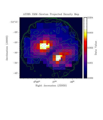
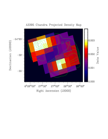
Figure 12: Projected density maps from 139 box regions using XMM-Newton data (top) and 42 box regions using Chandra data (bottom) with overlaid X-ray surface-brightness contours having levels same as in Figs. 2 and 4 respectively. The scales are expressed in units of cm^-3 shown in the bars alongside. Details of the spectral fittings are provided in §4.5.

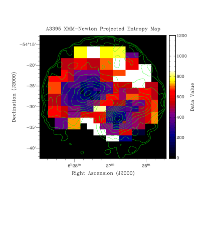
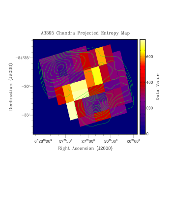
Figure 13: Projected entropy maps from 139 box regions using XMM-Newton data (top) and 42 box regions using Chandra data (bottom) with overlaid X-ray surface-brightness contours having levels same as in Figs. 2 and 4 respectively. The scales are expressed in units of keV cm² shown in the bars alongside. Details of the spectral fittings are provided in §4.5.

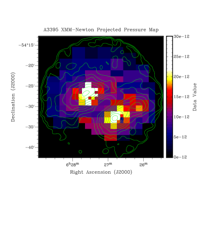
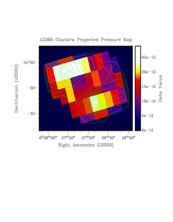
Figure 14: Projected pressure maps from 139 box regions using XMM-Newton data (top) and 42 box regions using Chandra data (bottom) with overlaid X-ray surface-brightness contours having levels same as in Figs. 2 and 4 respectively. The scales are expressed in units of erg cm^-3 shown in the bars alongside. Details of the spectral fittings are provided in §4.5.

$\begin{array}[]{ccc}\includegraphics[width=166.2212pt]{f18a.pdf}&\includegraphics[width=166.2212pt]{f18b.pdf}&\includegraphics[width=166.2212pt]{f18c.pdf}\end{array}$

Figure 18: Plots of the Newtonian energy binding conditions as a function of measured relative velocity ($V_{r}$) and projection angle from the plane of the sky ($\alpha$). The hyperbolic curve is the limiting case for bound systems i.e., all orbit solution above it are unbound while those below it are bound. The horizontal dashed line indicates the measured relative velocities of the subcluster pair and the cross-hatching shows its 68% confidence region.

References

- Abell et al. (1989) Abell, G. O., Corwin, H. G., Jr., & Olowin, R. P. 1989, ApJS, 70, 1
- Anders & Ebihara (1982) Anders, E., & Ebihara, M. 1982, Geochimica et Cosmochimica Acta, 46, 2363
- Angrick & Bartelmann (2011) Angrick, C., & Bartelmann, M. 2011, arXiv:1102.0458
- Beers et al. (1982) Beers, T. C., Geller, M. J., & Huchra, J. P. 1982, ApJ, 257, 23
- Blanton et al. (2003) Blanton, E. L., Gregg, M. D., Helfand, D. J., Becker, R. H., & White, R. L. 2003, AJ, 125, 1635
- Burgess & Hunstead (2006) Burgess, A. M., & Hunstead, R. W. 2006, AJ, 131, 100
- Burgett et al. (2004) Burgett, W. S., Vick, M. M., Davis, D. S., et al. 2004, MNRAS, 352, 605
- Burns (1981) Burns, J. O. 1981, MNRAS, 195, 523
- Burns et al. (1994) Burns, J. O., Rhee, G., Owen, F. N., & Pinkney, J. 1994, ApJ, 423, 94
- Carter & Read (2007) Carter, J. A., & Read, A. M. 2007, A&A, 464, 1155
- Domainko et al. (2005) Domainko, W., Kapferer, W., Schindler, S., et al. 2005, Advances in Space Research, 36, 685
- Donnelly et al. (2001) Donnelly, R. H., Forman, W., Jones, C., et al. 2001, ApJ, 562, 254
- Douglass et al. (2008) Douglass, E. M., Blanton, E. L., Clarke, T. E., Sarazin, C. L., & Wise, M. 2008, ApJ, 673, 763
- Dressler & Shectman (1988) Dressler, A., & Shectman, S. A. 1988, AJ, 95, 985
- Ehlert et al. (2011) Ehlert, S., Allen, S. W., von der Linden, A., et al. 2011, MNRAS, 411, 1641
- Eilek et al. (1984) Eilek, J. A., Burns, J. O., O’Dea, C. P., & Owen, F. N. 1984, ApJ, 278, 37
- Fabian (1994) Fabian, A. C. 1994, ARA&A, 32, 277
- Finoguenov et al. (2004) Finoguenov, A., Henriksen, M. J., Briel, U. G., de Plaa, J., & Kaastra, J. S. 2004, ApJ, 611, 811
- Flin (2003) Flin, P. 2003, Astronomical and Astrophysical Transactions, 22, 841
- Flin & Krywult (2006) Flin, P., & Krywult, J. 2006, A&A, 450, 9
- Forman & Jones (1990) Forman, W., & Jones, C. 1990, Clusters of Galaxies, 257
- Gardner et al. (1969) Gardner, F. F., Morris, D., & Whiteoak, J. B. 1969, Australian Journal of Physics, 22, 79
- Geller & Beers (1982) Geller, M. J., & Beers, T. C. 1982, PASP, 94, 421
- Gitti et al. (2010) Gitti, M., O’Sullivan, E., Giacintucci, S., et al. 2010, ApJ, 714, 758
- Girardi et al. (1997) Girardi, M., Escalera, E., Fadda, D., et al. 1997, ApJ, 482, 41
- Gregorini et al. (1994) Gregorini, L., de Ruiter, H. R., Parma, P., et al. 1994, A&AS, 106, 1
- Gregory et al. (1994) Gregory, P. C., Vavasour, J. D., Scott, W. K., & Condon, J. J. 1994, ApJS, 90, 173
- Gomez et al. (1997) Gomez, P. L., Pinkney, J., Burns, J. O., et al. 1997, ApJ, 474, 580
- Gu et al. (2010) Gu, L.-Y., Wang, Y., Gu, J.-H., et al. 2010, Research in Astronomy and Astrophysics, Volume 10, Issue 10, pp. 1005-1012 (2010)., 10, 1005
- Gutierrez & Krawczynski (2005) Gutierrez, K., & Krawczynski, H. 2005, ApJ, 619, 161
- Henry et al. (2004) Henry, J. P., Finoguenov, A., & Briel, U. G. 2004, ApJ, 615, 181
- Henriksen & Jones (1996) Henriksen, M., & Jones, C. 1996, ApJ, 465, 666
- Jaffe & Perola (1973) Jaffe, W. J., & Perola, G. C. 1973, A&A, 26, 423
- Jones & Forman (1992) Jones, C., & Forman, W. 1992, NATO ASIC Proc. 366: Clusters and Superclusters of Galaxies, 49
- Jones & Forman (1999) Jones, C., & Forman, W. 1999, ApJ, 511, 65
- Jones & McAdam (1992) Jones, P. A., & McAdam, W. B. 1992, ApJS, 80, 137
- Kalberla et al. (2005) Kalberla, P. M. W., Burton, W. B., Hartmann, D., et al. 2005, A&A, 440, 775
- Kauffmann & White (1993) Kauffmann, G., & White, S. D. M. 1993, MNRAS, 261, 921
- Kellogg et al. (1972) Kellogg, E., Gursky, H., Tananbaum, H., Giacconi, R., & Pounds, K. 1972, ApJ, 174, L65
- Klamer et al. (2004) Klamer, I., Subrahmanyan, R., & Hunstead, R. W. 2004, MNRAS, 351, 101
- Kriessler & Beers (1997) Kriessler, J. R., & Beers, T. C. 1997, AJ, 113, 80
- Large et al. (1981) Large, M. I., Mills, B. Y., Little, A. G., Crawford, D. F., & Sutton, J. M. 1981, MNRAS, 194, 693
- Mao et al. (2009) Mao, M. Y., Johnston-Hollitt, M., Stevens, J. B., & Wotherspoon, S. J. 2009, MNRAS, 392, 1070
- Mao et al. (2010) Mao, M. Y., Sharp, R., Saikia, D. J., et al. 2010, MNRAS, 406, 2578
- Markevitch et al. (1998) Markevitch, M., Forman, W. R., Sarazin, C. L., & Vikhlinin, A. 1998, ApJ, 503, 77
- Markevitch & Vikhlinin (2007) Markevitch, M., & Vikhlinin, A. 2007, Phys. Rep., 443, 1
- Maurogordato et al. (2011) Maurogordato, S., Sauvageot, J. L., Bourdin, H., et al. 2011, A&A, 525, A79
- McNamara & Nulsen (2007) McNamara, B. R., & Nulsen, P. E. J. 2007, ARA&A, 45, 117
- Mitchell et al. (1979) Mitchell, R. J., Dickens, R. J., Burnell, S. J. B., & Culhane, J. L. 1979, MNRAS, 189, 329
- Moffet (1975) Moffet, A. T. 1975, Galaxies and the Universe, 211
- Morrison & McCammon (1983) Morrison, R., & McCammon, D. 1983, ApJ, 270, 119
- Murgia et al. (1999) Murgia, M., Fanti, C., Fanti, R., et al. 1999, A&A, 345, 769
- Nakamura et al. (1995) Nakamura, F. E., Hattori, M., & Mineshige, S. 1995, A&A, 302, 649
- O’Donoghue et al. (1990) O’Donoghue, A. A., Owen, F. N., & Eilek, J. A. 1990, ApJS, 72, 75
- O’Sullivan et al. (2010) O’Sullivan, E., Giacintucci, S., David, L. P., Vrtilek, J. M., & Raychaudhury, S. 2010, MNRAS, 407, 321
- Owers et al. (2011) Owers, M. S., Randall, S. W., Nulsen, P. E. J., et al. 2011, ApJ, 728, 27
- Randall et al. (2008) Randall, S., Nulsen, P., Forman, W. R., et al. 2008, ApJ, 688, 208
- Reid (2000) Reid, A. D. 2000, PASA, 17, 285
- Richstone et al. (1992) Richstone, D., Loeb, A., & Turner, E. L. 1992, ApJ, 393, 477
- Roettiger et al. (1996) Roettiger, K., Burns, J. O., & Loken, C. 1996, ApJ, 473, 651
- Sakelliou & Merrifield (2000) Sakelliou, I., & Merrifield, M. R. 2000, MNRAS, 311, 649
- Sarazin (1988) Sarazin, C. L. 1988, Cambridge Astrophysics Series, Cambridge: Cambridge University Press, 1988,
- Sault et al. (1995) Sault, R. J., Teuben, P. J., & Wright, M. C. H. 1995, Astronomical Data Analysis Software and Systems IV, 77, 433
- Schuecker et al. (2001) Schuecker, P., Böhringer, H., Reiprich, T. H., & Feretti, L. 2001, A&A, 378, 408
- Smith et al. (2001) Smith, R. K., Brickhouse, N. S., Liedahl, D. A., & Raymond, J. C. 2001, ApJ, 556, L91
- Snowden et al. (2008) Snowden, S. L., Mushotzky, R. F., Kuntz, K. D., & Davis, D. S. 2008, A&A, 478, 615
- Strüder et al. (2001) Strüder, L., Briel, U., Dennerl, K., et al. 2001, A&A, 365, L18
- Teague et al. (1990) Teague, P. F., Carter, D., & Gray, P. M. 1990, ApJS, 72, 715
- Tittley & Henriksen (2001) Tittley, E. R., & Henriksen, M. 2001, ApJ, 563, 673
- Turner et al. (2001) Turner, M. J. L., Abbey, A., Arnaud, M., et al. 2001, A&A, 365, L27
- Wall et al. (1975) Wall, J. V., Shimmins, A. J., & Bolton, J. G. 1975, Australian Journal of Physics Astrophysical Supplement, 34, 55
- Weratschnig (2010) Weratschnig, J. 2010, Mem. Soc. Astron. Italiana, 81, 163
- Worrall (2009) Worrall, D. M. 2009, A&A Rev., 17, 1
- Wright et al. (1994) Wright, A. E., Griffith, M. R., Burke, B. F., & Ekers, R. D. 1994, ApJS, 91, 111
- Wright & Otrupcek (1990) Wright, A., & Otrupcek, R. 1990, PKS Catalog (1990), 0
- Xue & Wu (2000) Xue, Y.-J., & Wu, X.-P. 2000, ApJ, 538, 65