Measuring Expansion Velocities in Type II-P Supernovae

Abstract

We estimate photospheric velocities of Type II-P supernovae using model spectra created with SYNOW, and compare the results with those obtained by more conventional techniques, such as cross-correlation, or measuring the absorption minimum of P Cygni features. Based on a sample of 81 observed spectra of 5 SNe, we show that SYNOW provides velocities that are similar to ones obtained by more sophisticated NLTE modeling codes, but they can be derived in a less computation-intensive way. The estimated photopheric velocities ($v_{model}$) are compared to ones measured from Doppler-shifts of the absorption minima of the H$\beta$ and the Fe ii $\lambda 5169$ features.

Our results confirm that the Fe ii velocities ($v_{Fe}$) have tighter and more homogeneous correlation with the estimated photospheric velocities than the ones measured from H$\beta$, but both suffer from phase-dependent systematic deviations from those. The same is true for comparison with the cross-correlation velocities. We verify and improve the relations between $v_{Fe}$, $v_{H\beta}$ and $v_{model}$ in order to provide useful formulae for interpolating/extrapolating the velocity curves of Type II-P SNe to phases not covered by observations. We also discuss the implications of our results for the distance measurements of Type II-P SNe, and show that the application of the model velocities is preferred in the Expanding Photosphere Method.

1 Introduction

Type II-P supernovae (SNe) are core-collapse (CC) induced explosions that eject massive hydrogen-rich envelope. These SNe show a nearly constant-luminosity plateau in their light curve. The plateau phase lasts for $\sim$100 days, and finally ends up in a rapid decline of the luminosity as the expanding ejecta becomes fully transparent.

CC SNe and their progenitors play important role in understanding the evolution of the most massive stars. Extensive searches for SN progenitors showed that the progenitors of Type II-P SNe are stars with initial masses between $\sim$ 8 and 17 M_⊙ (Smartt et al., 2009). The lower value is roughly in agreement with the prediction of current theoretical evolutionary tracks, but the upper limit is somewhat lower than expected. The fate of the more massive (M $\geq$ 20 M_⊙) stars is controversial. They are thought to be the input channel for Type Ib/c SNe (Gaskell et al, 1986), but this has not been confirmed directly by observations yet (Smartt, 2009).

Any observational study of the physics of SNe and their progenitors (and, obviously, all astronomical objects) depends heavily on the knowledge of their distances. Because distance is such a crucial parameter, strong efforts have been devoted to the development of distance measurement techniques that are applicable for Type II-P SNe.

The Expanding Photosphere Method (EPM) (Kirshner & Kwan, 1974), a variant of the Baade-Wesselink method, uses the idea of comparing the angular and the physical diameter of the expanding SN ejecta. The input quantities are fluxes, temperatures and velocities observed at several epochs during the photospheric phase. Thus, EPM requires both photometric and spectroscopic monitoring of SNe throughout the plateau phase. A clear advantage of EPM is that it does not require external calibration via SNe with known distances. Another interesting property is that EPM is much less sensitive to uncertainties in the interstellar reddening and absorption toward SNe. As Eastman, Schmidt & Kirshner (1996) (hereafter E96) have shown, 1 mag uncertainty in $A_{V}$ results in only $\sim 8$ % error in the derived distance. However, the assumption that the SN atmosphere radiates as a blackbody diluted by electron scattering raised some concerns. These led to the development of the applications of full NLTE model atmospheres, like the PHOENIX code in the “Spectral-fitting Expanding Atmosphere Method” (SEAM) (Baron et al., 2004), or the CMFGEN code by Dessart & Hillier (2005a); Dessart & Hillier (2005b). The drawback of these approaches is that the building of tailored model atmospheres can be very time-consuming and needs much more computing power. Also, in order to compute reliable models, the input observed spectra need to have sufficiently high S/N and spectral resolution.

The more recently developed Standardized Candle Method (SCM) (Hamuy & Pinto, 2002; Hamuy et al., 2003) relies on the empirical correlation between the measured expansion velocity and the luminosity in optical (Nugent et al., 2006; Poznanski et al., 2009) or in NIR (Maguire et al., 2010a) bands in the middle of plateau phase, at +50 days after explosion. This method requires less extensive input data, but needs a larger sample of Type II SNe with independently known distances in order to calibrate the empirical correlation. Because this is basically a photometric method which compares apparent and absolute magnitudes, SCM is more sensitive to interstellar reddening than EPM/SEAM, as mentioned above.

Beside photometry, both EPM/SEAM and SCM need information on the expansion velocity at the photosphere ($v_{phot}$). At first, EPM seems to be more challenging, because it requires multi-epoch observations, while SCM needs only the velocity at a certain epoch, at +50 days after explosion ($v_{50}$). However, direct measurement of $v_{50}$ is possible only in the case of precise timing of the spectroscopic observation, which is rarely achievable.

The correct determination of $v_{phot}$ is not trivial. As SNe expand homologously ($v\sim r$, where $v$ is the velocity of a given layer and $r$ is its distance from the center), in most cases it is difficult to derive a unique velocity from the observed spectral features. The most frequently followed approach relies on measuring the Doppler-shift of the absorption minimum of certain spectral features (mostly Fe ii $\lambda 5169$ or H$\beta$). Another possibility is the computation of the cross-correlation between the SN spectrum and a set of spectral templates, consisting of either observed or model spectra, with known velocities. The third method is building a full NLTE model (like PHOENIX or CMFGEN) for a given SN spectrum, and adopting the theoretical $v_{phot}$ from the best-fitting model.

The aim of this paper is to present a similar, but less computation-demanding approach to assign velocities to observed SN spectra. We apply the simple parametrized code SYNOW (Fisher, 1999; Hatano et al., 1999) to model the observed spectra with an approximative, but self-consistent treatment of the formation of lines in the extended, homologously expanding SN atmosphere. To illustrate the applicability of SYNOW, we construct and fit parametrized models to a sample of five well-observed, nearby Type II-P SNe that have a series of high S/N spectra publicly available. We also check and re-calibrate some empirical correlations between velocities derived from various methods. The description of the observational sample is given in §2. In §3 we first review the different velocity measurement techniques for SNe II-P, then we present the details of the application of SYNOW models (§3.4). The results are collected and discussed in §4 and §5, while the implications of the results for the distance measurements are in §6. We draw our conclusions in §7.

2 Data

Our sample contains 81 plateau phase–spectra of five objects, SNe 1999em, 2004dj, 2004et, 2005cs and 2006bp, respectively. All five SNe are well-observed objects, they have been studied in detail, and show a wide variety in their physical properties (see Table 1).

Table 1: The physical properties of the supernovae used in this paper.

SN	t0	Distance	cz	E(B-V)	$M_{Ni}$	$M_{prog}$	References
	(JD-245000)	(Mpc)	(km s-1)	(mag)	($10^{-2}$ M⊙)	(M⊙)
SN 1999em	1477.0	7.5 – 12.5	717	0.10	2.2 – 3.6	$<$15	1,2,3,4,5,6,7,8
SN 2004dj	3187.0	3.2 – 3.6	131	0.07	1.3 – 2.2	12 – 20	9,10,11,12,13,14,15
SN 2004et	3270.5	4.7 – 6.0	48	0.41	5.6 – 6.8	9, 15 – 20	16,17,18,19,20,21,22
SN 2005cs	3549.0	7.1 – 8.9	463	0.05	0.3 – 0.8	6 – 13	23,24,25,26,27,28,29
SN 2006bp	3835.1	17.0 – 18.3	987	0.40	–	12 – 15	26,30

• ¹ NED, http://nedwww.ipac.caltech.edu/

• ² References: (1) Hamuy et al. (2001), (2) Leonard et al. (2002), (3) Smartt et al. (2002), (4) Leonard et al. (2003), (5) Elmhamdi et al. (2003), (6) Baron et al. (2004), (7) Dessart & Hillier (2006), (8) Utrobin (2007), (9) Maíz-Apellániz et al. (2004), (10) Kotak et al. (2005), (11) Wang et al. (2005), (12) Chugai et al. (2005), (13) Zhang et al. (2006), (14) Vinkó et al. (2006), (15) Vinkó et al. (2009), (16) Li et al. (2005), (17) Sahu et al. (2006), (18) Misra et al. (2007), (19) Utrobin & Chugai (2009), (20) Poznanski et al. (2009), (21) Maguire et al. (2010b), (22) Crockett et al. (2011), (23) Maund, Smartt & Danziger (2005), (24) Pastorello et al. (2006), (25) Takáts & Vinkó (2006), (26) Dessart et al. (2008), (27) Eldridge, Mattila & Smartt (2007), (28) Utrobin & Chugai (2008), (29) Pastorello et al. (2009), (30) Immler et al. (2007)

SN 1999em was discovered on 29th October 1999 by Li (1999) in NGC 1637 at a very early phase. It is a very well-observed, well-studied object The explosion date was determined as $2451477.0\pm 2$ JD (Leonard et al., 2002; Hamuy et al., 2001; Dessart & Hillier, 2006). We used the spectra of Leonard et al. (2002) and Hamuy et al. (2001) downloaded from the SUSPECT database. Our sample contains 22 spectra, covering the first 80 days of the plateu phase.

SN 2004dj was discovered on 31st July 2004 by Itagaki (Nakano et al., 2004) in a young, massive cluster Sandage-96 of NGC 2403, about 1 month after explosion. We used the spectra taken by Vinkó et al. (2006). Due to the lack of observed spectrophotometric standards, the flux-calibration of those spectra was inferior, but this is not a major concern when only velocities are to be determined. We included 12 spectra taken between +47 and +100 days after explosion in our sample.

SN 2004et was discovered by Moretti (Zwitter, Murani & Moretti, 2004) on 27th September 2004 in NGC 6946. The spectra of Sahu et al. (2006) (downloaded from SUSPECT) and Maguire et al. (2010b) were used, together with 6 previously unpublished early-phase spectra taken with the 1.88-m telescope at DDO (see the Appendix A). The 22 spectra cover the period of $+$11 to $+$104 days after explosion.

SN 2005cs was discovered on 29th June 2005 by Kloehr (2005) in M51. Due to its very early discovery and proximity, this object is very well-sampled and studied in detail. It is a underluminous, low-energy, Ni-poor SN that had a low-mass progenitor (see Table 1 for references). 14 spectra of Pastorello et al. (2006) and Pastorello et al. (2009) were used, which were obtained between days +3 and +61.

SN 2006bp was discovered on 9th April 2006 by (Nakano & Itagaki, 2006) in NGC 3953, also in a very early phase. We used 11 spectra of Quimby et al. (2007), downloaded from SUSPECT, covering the period between $+$5 and $+$72 days.

3 The issue of measuring expansion velocities in SNe

During the photospheric phase the homologously expanding Type II-P SN ejecta consist of two parts: the outer, partly transparent atmosphere where the observable spectral features are formed, and an optically thick inner part, which emits most of the continuum radiation as a “diluted” blackbody (e.g. E96). Because the inner part is mostly ionized, the major source of the total opacity is electron scattering. Thus, the instantaneous photosphere is located at the depth where the outgoing photons are last scattered, i.e. where the electron-scattering optical depth is $\tau_{e}\sim 2/3$ (Dessart & Hillier, 2005a, hereafter D05). This is presumed to occur in a thin, spherical shell at a certain radius $r_{phot}$, and the homologous expansion gives this a unique velocity $v_{phot}=v_{ref}\cdot r_{phot}/r_{ref}$, where $r_{ref}$ is the radius of an (arbitrary) reference layer and $v_{ref}$ is its expansion velocity. As the ejecta expands and dilutes, the photosphere migrates inward, toward the inner layers of the ejecta that expand slower, thus, $v_{phot}$ continuously declines in time.

The issue of measuring $v_{phot}$ comes from the fact that no measurable spectral feature is connected directly to $v_{phot}$. As previously mentioned in §1, there exist several observational/theoretical approaches to estimate $v_{phot}$ from observed spectra. In the followings we briefly review these methods, summarizing their advantages/drawbacks.

3.1 P Cygni lines

The most widely used method is to measure the velocity represented by the minimum flux of the absorption component of an unblended P Cygni line profile (sometimes referred to as “maximum absorption”, $v_{abs}$, Dessart & Hillier, 2005b). This is motivated by the theory of P-Cygni line formation (e.g. Kasen et al., 2002), which predicts that the minimum flux in a P-Cygni line occurs at the velocity of the photosphere. Strictly speaking, this is only true for an optically thin line formed by pure scattering. In most cases the Fe ii $\lambda 5169$ feature is used for measuring $v_{abs}$, for which Dessart & Hillier (2005b) pointed out that it can represent the true $v_{phot}$ within 5 – 10 % accuracy. However, Leonard et al. (2002) showed that using weaker, unblended features one can get $\sim 10$ % lower velocities than from the Fe ii $\lambda 5169$ feature. This raises the question of whether the measurable lines were indeed optically thin and unblended, and which one represented the true $v_{phot}$. Moreover, Dessart & Hillier (2005b) also revealed that $v_{abs}$ can either over- or underestimate $v_{phot}$, depending on various physical conditions, like the density gradient and the excitation/ionization conditions for the particular transition within the ejecta.

While the Fe ii $\lambda 5169$ feature can be relatively easily identified and measured in Type II-P SNe spectra obtained later than $\sim 20$ days after explosion (which is undoubtedly a major advantage of this method), this is not so for earlier phases. In early-phase spectra only the Balmer-lines and maybe He i features (mostly the $\lambda 5876$ feature) can be identified. These features are less useful for measuring $v_{phot}$, because none of them are optically thin, and the He i $\lambda 5876$ feature can sometimes be blended with Na i D. Moreover, their line profile shapes often make the location of the minimum of absorption component difficult to determine (Dessart & Hillier, 2005b, 2006).

Also, in spectra having less signal-to-noise, the weaker Fe ii features are often buried in the noise, making them inappropriate for velocity measurement. In these cases several authors attempted to use the stronger features, especially $H\beta$. Although Dessart & Hillier (2005b) pointed out that $v_{H\beta}$ is certainly less tightly connected to $v_{phot}$ than the weaker Fe ii $\lambda 5169$ feature, Nugent et al. (2006) have shown that the ratio $v_{H\beta}/v_{Fe}$ is $\sim 1.4$ below $v_{H\beta}=6000$ km s^-1, and it is linearly decreasing for higher velocities. Recently this correlation was revised by Poznanski, Nugent & Filippenko (2010) by revealing an entirely linear relation between $v_{H\beta}$ and $v_{Fe}$, but restricting the analysis only for velocities measured between +5 and +40 days after explosion. The uncertainty of estimating $v_{Fe}$ from $v_{H\beta}$ is $\sim 300$ km s^-1 (Poznanski et al., 2010). It is emphasized that these empirical relations are more-or-less valid between the velocities of two observable features, but both of them may be systematically off from the true $v_{phot}$. Indeed, Dessart & Hillier (2005b) found that $v_{H\beta}$ can be either higher or lower than $v_{phot}$ with an overall scattering of $\pm 15$ %. For velocities below 10,000 km s^-1 $v_{H\beta}$ is usually higher than $v_{phot}$, in accord with the empirical correlations with $v_{Fe}$, but above 10,000 km s^-1 it can be lower than $v_{phot}$.

3.2 Cross-correlation

Figure 1: Model spectra of a Type II-P SN in early-phase (top left) and late-phase (top right), and the resulting CCFs (bottom panels) after cross-correlating the spectra with their identical models but having 2000 km s^-1 higher $v_{phot}$. The arrows mark the peak location of the CCFs, while the true relative velocity difference $\Delta v_{phot}$ is indicated by the dotted vertical line. The peak of the CCF underestimates $\Delta v_{phot}$ in both cases.

Motivated by the uncertainties of measuring the Doppler-shift of a single, weak feature in a noisy spectrum, several authors proposed the usage of the cross-correlation technique, which is a powerful method for measuring Doppler-shifts of stellar spectra containing many narrow spectral features. This method predicts the Doppler-shift of the entire spectrum by computing the cross-correlation function (CCF) between the observed spectrum and a template spectrum with a-priori known velocity $v_{templ}$. The resulting velocity is $v_{cc}=v_{rel}+v_{templ}$, where $v_{rel}$ is the velocity where the CCF reaches its maximum (i.e. the relative Doppler-shift between the observed spectrum and the template).

However, the applicability of cross-correlation for SN spectra is not obvious, because of the physics of P Cygni line formation in SN atmospheres. If $v_{phot}$ is higher, then the center of the absorption component gets blueshifted, while the center of the emission component stays close to zero velocity. Thus, cross-correlating two spectra with different $v_{phot}$, the relative velocity will underestimate the true velocity difference between the two spectra. This is illustrated in Fig. 1, where we determined the CCF between two Type II-P SN model spectra (computed with SYNOW, see below) that were identical except their $v_{phot}$ which differed by $\Delta v_{phot}=2000$ km s^-1. The cross-correlation was computed only in the 4500 - 5500 Å  interval to exclude the $H\alpha$ feature. This was done for an early-phase spectrum containing only H and He features (Fig. 1 left panel) and a later-phase spectrum with more developed metallic lines (Fig. 1 right panel). It is visible in the bottom panels that the maximum of the CCF (i.e. $v_{rel}$) is shifted toward lower velocities with respect to the true $\Delta v_{phot}$ (indicated by a dotted vertical line in the CCF plot) for both spectra. The systematic offset of $v_{rel}$ from $\Delta v_{phot}$ is $\sim 200$ km s^-1 for the later-phase spectrum that contains many narrower absorption features, and it reaches $\sim 700$ km s^-1 for the early-phase spectrum that are dominated by broad Balmer lines with stronger emission component. These simple tests are in very good agreement with the results of Hamuy et al. (2001) and Hamuy (2002), who applied the cross-correlation technique using model spectra of E96 with a-priori known $v_{phot}$ as templates. They pointed out that $v_{rel}$ usually underestimates $\Delta v_{phot}$ so that $\Delta v_{phot}/v_{rel}\sim 1.18$, with the scatter of $\sim 900$ km s^-1.

Another variant of the CCF method was proposed by Poznanski et al. (2009), and it was also applied by D’Andrea et al. (2010) and Poznanski et al. (2010). They took their template spectra from the library of the SuperNova IDentification code SNID (Blondin & Tonry, 2007) that contains high S/N observed spectra of many SNe, but used only those templates that showed well-developed Fe ii $\lambda 5169$ feature. The reason for their choice was that they wanted to estimate $v_{Fe}$ at +50 days after explosion ($v_{50}$), which is an input parameter in SCM. This template selection caused the well-known issue of template mismatch that further biases the cross-correlation results. As D’Andrea et al. (2010) concluded, this template mismatch can result in significant underestimate of $v_{Fe}$ by $\sim 1500$ km s^-1 for spectra obtained at $t<20$ days, and is also present in later-phase specta, although being less pronounced, $\sim 300-400$ km s^-1. To overcome this problem, in a subsequent paper Poznanski et al. (2010) suggested the application of their $v_{Fe}$ vs. $v_{H\beta}$ relation to estimate $v_{Fe}$ by measuring $v_{H\beta}$ for these early-phase spectra and then propagate the resulting velocity to day +50. Nevertheless, the two groups presented velocities that were different by $200$ to $1000$ km s^-1 for the same set of SNe spectra from the SDSS-II survey. This underlines that although cross-correlation seems to be an easy and robust method that gives reasonable velocities even for low S/N spectra, the results may be heavily biased, especially at early phases, when the SN spectra contain only a few, broad features.

3.3 Tailored modeling

Tailored modeling of the whole observed spectrum via NLTE models were invoked e.g. by Baron et al. (2004) using the code PHOENIX, and Dessart & Hillier (2006) and Dessart et al. (2008) with the code CMFGEN. Here $v_{phot}$ is determined implicitly by requiring an overall fit of the entire observed spectrum by a synthetic spectrum from a full NLTE radiation-hydrodynamics model. In these models the location of the photosphere is usually defined as the layer where the electron scattering optical depth reaches unity or 2/3 (e.g. D05). $v_{phot}$ is then simply determined by the radius $r_{phot}$ and the law of homologous expansion (see above). Although this is probably the best self-consistent method for obtaining SN velocities, building full NLTE models for multiple epochs requires a lot of computing power. Thus, its usage for a larger sample of SNe would be very time-consuming and impractical. Also, in some cases a good global fit to the whole spectrum may not be equally good for individual spectral lines, where lots of physical details play important role in the formation of the given features. This may lead to some uncertainties in the velocities given by the models, which will be illustrated in § 4.

3.4 Using SYNOW

The success of tailored spectrum models to estimate $v_{phot}$ suggests a similar, but much more simplified approach: the usage of parametrized spectrum models that do not contain the computation-intensive details of NLTE level populations or exact radiative transfer calculations, but preserve the basic physical assumptions of an expanding SN atmosphere, and able to reproduce the formation of P Cygni lines in a simplified manner. Such models can be computed either with the SYNOW code (Branch et al., 2002), or the more recently developed SYNAPPS code (Thomas, Nugent, & Meza, 2011) that has a parameter-optimizer routine built-in. In this paper we apply SYNOW to calculate model spectra. Because SYNOW does only spectrum synthesis and has no fitting capabilities, we used self-developed UNIX shell scripts to fine-tune the parameters until a satisfactory fit to the observed spectrum is achieved.

The basic assumptions of SYNOW are the followings: $i)$ the SN ejecta expand homologously; $ii)$ the photosphere radiates as a blackbody; $iii)$ spectral lines are formed entirely above the photosphere; $iv)$ the line formation is due to pure resonant scattering. Level populations are treated in LTE, and the radiative transfer equation is solved in the Sobolev approximation (see also in e.g. Kasen et al., 2002).

When running SYNOW, several parameters must be set. These are the temperature of the blackbody radiation ($T_{bb}$) emitted by the photosphere, the expansion velocity at the photosphere ($v_{phot}$), the chemical composition of the ejecta and the optical depth of a reference line ($\tau_{ref}$) of each compound. For each atom/ion the optical depths for the rest of the lines are calculated assuming Boltzmann excitation governed by the excitation temperature $T_{exc}$. The location of the line-forming region in the atmosphere can be tuned for each compound by setting the velocities of the lower and upper boundary layers, $v_{min}$ and $v_{max}$. The optical depth as a function of velocity (i.e. radius) can be modeled either as a power-law, or an exponential function. We assumed power-law atmospheres, and adjusted the power-law exponent $n$ to reach optimal fitting.

After setting the inital values by hand, several models in a wide range of $v_{phot}$, $n$, and $\tau_{ref}$ were created for a pre-selected set of ions. In order to reduce the number of free parameters, we initially set $T_{bb}$ (which has very little effect on the line shapes) to represent the continuum of the fitted spectrum and kept it fixed during the optimization. Moreover, we applied a single power-law exponent $n$ for all atoms/ions. We also assumed that all spectral features are photospheric, thus, fixing $v_{min}$ well below the photosphere and $v_{max}$ at $\sim 40000$ km s^-1.

The best-fitting model was then chosen via $\chi^{2}$-minimization, and the fitting process was iterated for a few times, each time resampling the parameter grid in the vicinity of the minimum of the $\chi^{2}$ function found in the previous iteration cycle. This way we determined the parameters and the chemical compositions that best describe the observed spectra.

Then, to further refine the estimated photospheric velocity, we fine-tuned only $v_{phot}$ of the best-fitting model, and calculated the $\chi^{2}$ function only in the vicinity of certain lines instead of the whole spectrum. This may reduce the systematic under- or overestimate of $v_{phot}$ produced by false positive fitting to the observed spectrum outside the range of the considered spectral features.

Motivated by the results of Dessart & Hillier (2005b) (see §3.1), we have chosen the Fe ii $\lambda 5169$ feature for this fine-tuning process. When this feature was not present in the observed spectrum (i.e. the early-phase spectra, before $\sim$15 days) we used H$\beta$ (see §3.1) instead. Hereafter we denote the $v_{phot}$ parameter of the best-fitting SYNOW model as $v_{model}$. Errors of $v_{model}$ were estimated by choosing the 90 % confidence interval around the minimum of the $\chi^{2}$ function.

Fig. 2 shows two examples for an early- and a later-phase spectrum of SN 1999em together with the best-fitting model. The right panel zooms in on the region of H$\beta$ and Fe ii $\lambda 5169$. Note that although the final fitting was restricted to the proximity of these lines, the best model describes the entire observed spectrum (except H$\alpha$) very well.

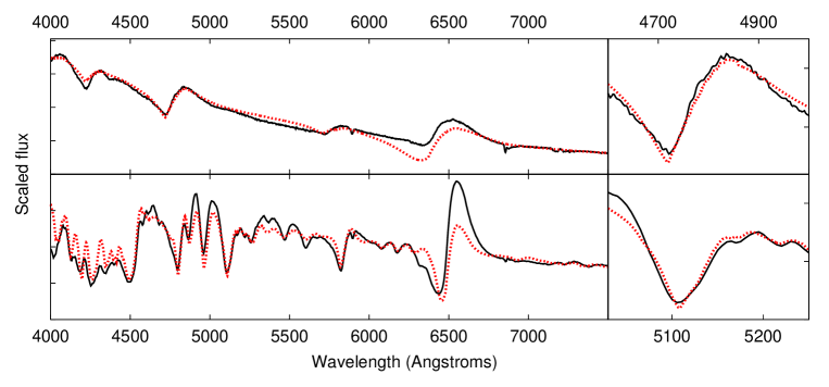
Figure 2: The observed (black solid line) and best-fitting model (red dashed line) spectra of SN 1999em on days $+$9 (top) and $+$41 (bottom). The right panels enlarge the wavelength regions of the fitted lines: H$\beta$ (top) and Fe ii $\lambda 5169$ (bottom).

This velocity measurement method have multiple sources of error. One of them may be the systematic bias due the approximations in the model (LTE, power-law atmosphere, simple source function, etc.). However, the comparison of our results with those from full NLTE CMFGEN models (§4) show no systematic bias in the case of SNe 1999em and 2005cs. The agreement between the velocities from these two very different modeling codes are within $\pm 10$ percent. For SN 2006bp the differences are higher, but it will be shown below that for this SN the CMFGEN models do not describe well the spectral features we use, contrary to the SYNOW models (§4.5).

Another source of error may be the correlation between the parameters. In Fig. 3 we present contour plots of the $\chi^{2}$ hyperspace around its minimum, as a function of $v_{model}$ and several other parameters that can affect the shape of the fitted Fe ii $\lambda 5169$ feature. The thick black contour curve corresponds to 50 % higher $\chi^{2}$ than the minimum value. It is visible that correlation is indeed present (i.e. the contours are distorted) between $v_{model}$ and the power-law exponent $n$ or the optical depth $\tau_{Fe}$. The correlation is much less between $v_{model}$ and $\tau_{ref}$ of Ti ii and Mg i, whose features may blend with Fe ii $\lambda 5169$. However, even for the correlated parameters, selecting $n$ or $\tau_{Fe}$ very far from their optimum value can alter $v_{model}$ only by a few hundred km s^-1. Thus, we conclude that uncertainties in finding the minimum of $\chi^{2}$ do not cause errors in $v_{model}$ that significantly exceed the uncertainty due to the spectral resolution of the observed spectra (which is usually between 200 - 300 km s^-1).

A possible source of uncertainty may be that during the final fitting the wavelength interval around the used spectral feature is chosen somewhat subjectively. However, our tests showed that changing the limits reasonably has negligible effect on the final velocities.

It is emphasized that although the final fitting is restricted to a vicinity of a well-defined spectral line, this method is certainly more reliable than the measurement of only the location of the minimum of the same feature. As it was discussed above, the minimum can be significantly and systematically altered by signal-to-noise, spectral resolution, blending, etc. The fitting of a model spectrum to the entire feature is expected to overcome these difficulties, provided the underlying model is not too far from reality.

Figure 3: Contour plot of the $\chi^{2}$ function around its minimum, as a function of $v_{model}$ and power-law exponent $n$ (a), $\tau_{ref}$ of Fe ii (b), Ti ii (c) and Mg i (d). The thick black contour curve corresponds to 50 % higher $\chi^{2}$ than the minimum value. The parameters plotted in (a) and (b) are definitely correlated, while the correlation is much less between the parameters in the (c) and (d) panels.

4 Comparing the results from different methods

Using SYNOW as described above, we determined the best-fitting parameters of all SNe spectra from Sec. 2. The resulting model velocities are collected in Table 5 in Appendix B. The best-fitting SYNOW parameters, such as $\tau_{ref}$ for each atom/ion, the power-law exponent $n$ and $v_{model}$ together with the chosen $T_{phot}$, can be found in Table 6 in Appendix C. In Table 5 we also list the $v_{Fe}$ and $v_{H\beta}$ velocities. For SNe 1999em, 2005cs and 2006bp, we collected the photospheric velocities from $\tt CMFGEN$ models of Dessart & Hillier (2006) and Dessart et al. (2008). These are included in Table 5 as $v_{nlte}$. Velocities from the cross-correlation technique (Sect. 3.2) were obtained using two sets of template spectra. The first set contained the 22 observed spectra of SN 1999em (set #1), while the second set was based on the $\tt CMFGEN$ models mentioned above (set #2). The velocities of the template spectra were $v_{Fe}$ for set #1 and $v_{nlte}$ for set #2. We cross-correlated all the observed spectra with the two sets separately on the wavelength range of 4500 – 5500 Å, and the resulting velocities are also in Table 5 as $v_{cc}$.

Fig. 4 shows $v_{model}$ against phase for all studied SNe (top left panel), and the ratio of $v_{model}$ to all the other velocities. The calculated velocities all show the expected decline with phase as the photosphere moves deeper and deeper within the ejectra, toward slower expanding layers.

Similar plots containing the ratio $v_{model}/v_{cc}$ and $v_{abs}/v_{cc}$ as functions of phase, are presented in Fig. 5.

In the followings we provide some details of deriving these velocities for each object and discuss some object-specific differences between them.

4.1 SN 1999em

When determining $v_{model}$ with SYNOW, $H\beta$ was fitted for the first 6 spectra, then the Fe ii $\lambda 5169$ feature was used for the remaining 16 spectra. The resulting velocities are between $11000$ and $1800$ km s^-1. As seen in the bottom right panel of Fig. 4, $v_{model}$ and $v_{H\beta}$ are about the same for the early phases (before the appearance of the Fe ii lines), while later $v_{H\beta}$ tends to be higher than $v_{model}$. Also, between day +15 and day +40, $v_{model}$ is a slightly higher than $v_{Fe}$ (Fig. 4 bottom left panel). After day +40 $v_{model}$ drops below $v_{Fe}$ and their ratio increases toward later phases.

The velocities from CMFGEN models of (Dessart & Hillier, 2006) (Fig. 4 top right panel) agree with $v_{model}$. The cross-correlation with set #2 (Fig.5 bottom panels) gave similar results for the first few points, but overestimate $v_{model}$ between days +22 and +80. They mostly fall between $v_{H\beta}$ and $v_{Fe}$, which is expected, since we cross-correlated the range of 4500 – 5500 Å, where these features appear.

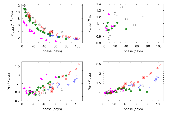
Figure 4: Top left panel: model velocities ($v_{model}$) from SYNOW as functions of phase. Top right panel: the ratio of SYNOW and CMFGEN model velocities ($v_{model}/v_{nlte}$) against phase. Bottom panels: The phase dependence of $v_{Fe}/v_{model}$ (bottom left) and $v_{H\beta}/v_{model}$ (bottom right). Different symbols code the followings: filled circles – SN 1999em; open circles – SN 2006bp; filled triangles – SN 2005cs; open triangles – SN 2004dj; asterisks – SN 2004et.

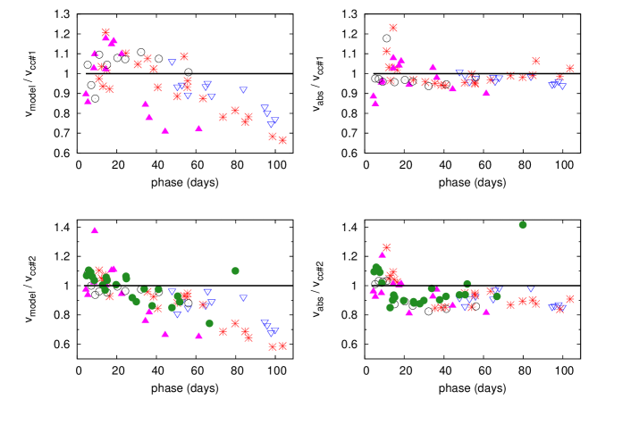
Figure 5: Top panels: Ratio of $v_{model}$ and $v_{abs}$ to $v_{cc}$ from cross-correlating with the observed spectra of SN 1999em (set #1, see text) as functions of phase. Bottom panels: the same as above, but with respect to the template set containing CMFGEN models (set #2). The symbols code the same SNe as in Fig.4.

4.2 SN 2004dj

The SYNOW model velocities of the 11 spectra that cover the second half of the plateau phase are between $\sim$ 3400 and 1700 km s^-1. These are similar to those of SN 1999em at the same phase. Both $v_{Fe}$ and $v_{H\beta}$ are higher than $v_{model}$ at all epochs, especially the latter with a factor of about $1.8$ (Fig. 4).

No CMFGEN model was available for SN 2004dj. Cross-correlation with both template sets gave very similar results. They are only slightly higher than both $v_{model}$ and $v_{Fe}$ (Fig.5).

4.3 SN 2004et

For the first 6 spectra the SYNOW model was optimized for $H\beta$, then for the Fe ii $\lambda 5169$ feature. The resulting model velocities are between 9700 and 1800 km s^-1 (Fig. 4). The $v_{Fe}$ values are similar to $v_{model}$, but their ratio shows slight phase dependence, similar to the other SNe studied here. On the contrary, the values of $v_{H\beta}$ are very different from $v_{model}$. At early phases they are close to $v_{model}$ (except for the first point), but later the $v_{H\beta}$ to $v_{model}$ ratio strongly increases, becoming as high as $2.5$.

Again, there is no CMFGEN model available for this SN. Cross-correlation with set #1 resulted in velocities similar to $v_{H\beta}$ at early phases and to $v_{Fe}$ later. With set #2, cross-correlation gave similar results at early phases, but later it produced systematically higher velocities. This underlines the importance of selecting proper template spectra and template velocities when applying the cross-correlation technique.

4.4 SN 2005cs

We used the H$\beta$ line for fitting the first 3 spectra with SYNOW. The velocities of this SN are very low: they are in the range of 7100 – 1100 km s^-1 and decrease quickly. The velocities from absorption minima are very close to $v_{model}$ for both H$\beta$ and Fe ii $\lambda 5169$. The $v_{Fe}$ values follow the tendency similar to the previous objects: they are somewhat lower than $v_{model}$ at the early phases, but get higher after about day +30. The $v_{H\beta}$ values are much closer to $v_{model}$ than for the other SNe, and the $v_{H\beta}/v_{model}$ ratio stays about the same for all epochs (Fig. 4). The velocities of the CMFGEN models for SN 2005cs are the same as the $v_{model}$ values for all epochs, except for day +9. Cross-correlation with both template sets resulted in velocities close to $v_{Fe}$.

4.5 SN 2006bp

The results for SN 2006bp are controversial. Applying SYNOW, the H$\beta$ line was fitted for the first 4 of the 11 observed spectra, while Fe ii $\lambda 5169$ was used for the rest. The model velocities are between 12000 and 3800 km s^-1. Both $v_{Fe}$ and $v_{H\beta}$ follow the tendency shown by other SNe (Fig. 4).

On the contrary, unlike in the previous two cases, the velocities from the CMFGEN models differ significantly from our $v_{model}$ values. At early epochs this difference is much lower ($\sim 500-700$ km s^-1) being close to zero at day +15. After day +15 it gets higher reaching $\sim 1200$ km s^-1 on day +32. At later phases the difference decreases somewhat, but stays being significant.

Cross-correlating the same spectra with the CMFGEN models using the wavelength range of $4500-5500$ Å  resulted in velocities that are very close to $v_{model}$ (except for day +9). Using the #1 template set, the results agree well with $v_{Fe}$, or $v_{H\beta}$ at early epochs.

To examine the obvious controversy between the velocity of the CMFGEN models and all the others, we plotted the observed spectra and the best-fitting CMFGEN model on day +32 (when the differences are the highest) in Fig. 6. Zooming in on the range of $4500-5500$ Å  clearly shows that the model by Dessart et al. (2008) does not fit these spectral features well, leading to an underestimate of the velocity. Thus, we suspect that the velocity differences we found are probably due to the inferior fitting of the CMFGEN models to the SN 2006bp spectra.

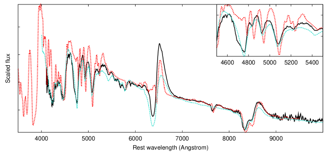
Figure 6: Plot of the CMFGEN (red dotted line) and the SYNOW models (turquoise dashed line) and the observed spectra (black continuous line) of SN 2006bp on day $+$ 32 (see text).

5 Discussion

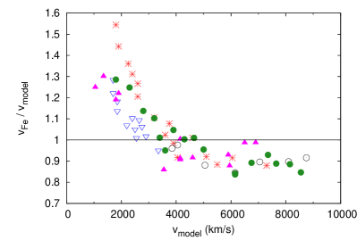
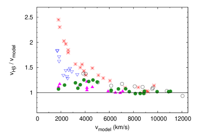
Figure 7: The $v_{Fe}/v_{model}$ (left panel) and $v_{H\beta}/v_{model}$ (right panel) ratio against the model velocities. The symbols have the same meaning as in Fig.4.

As shown in the previous sections, the photospheric velocities of four SNe in our sample evolved similarly. SNe 1999em, 2004et and 2006bp had high velocities at early phases and they decreased quickly, although their decline slopes were different. SN 2004dj probably showed similar evolution, but the lack of the early-phase data prevents a more detailed comparison. On the contrary, SN 2005cs was a very different, low-energy SN II-P as discussed in detail in previous studies. It had lower early velocities and the velocity curve decreased much faster than for all the other SNe.

As expected, the different velocity measurement methods we applied provided somewhat different results. As seen in Fig.5, the velocities obtained from cross-correlation are usually closer to $v_{abs}$ than to $v_{model}$. This is understandable, given that the cross-correlation method is most sensitive to the shapes and positions of the spectral features that may be biased toward lower, or higher velocities. The $v_{model}/v_{cc}$ ratio (Fig.5 top left and bottom left panels) shows the same trend (but plotted upside down) as the $v_{Fe}/v_{model}$ ratio in Fig.4 (bottom left panel), i.e. $v_{model}$ is higher between day 10 and 50, but becoming smaller than $v_{Fe}$ or $v_{cc}$. On the other hand, no such systematic trend can be identified between $v_{model}$ and $v_{nlte}$ (Fig.4, top right panel). These benchmarks suggest that the model velocities, either from SYNOW or CMFGEN are consistent, and they show phase-dependent offsets from the absorption minima, or cross-correlation velocities. The increasing systematic offset is particulary strong for $v_{H\beta}$ (Fig.4 bottom right panel). Thus, the traditional, simple measurement methods seem to underestimate the true photospheric velocities before day 50, but increasingly overestimate them toward later epochs. This should be kept in mind when the true photospheric velocities are needed, e.g. in the application of EPM.

In order to do further testing, we plotted the ratio of $v_{Fe}/v_{model}$ and $v_{H\beta}/v_{model}$ as a function of $v_{model}$ for all SNe, following Dessart & Hillier (2005b) (Fig. 7). The $v_{Fe}/v_{model}$ ratio shows the same trend for all objects: at high velocities (i.e. early phases) the ratio is somewhat lower than 1, then it reaches unity around $\sim 4000$ km s^-1, and below that it keeps rising, reaching $\sim$ 1.6 by the end of the plateau. The $v_{H\beta}/v_{model}$ ratio is more complicated. At high $v_{model}$ values it is around 1, but becomes higher than unity around $v_{model}\approx 7000$ km s^-1. Below that the slope of the rising changes from object to object. In the case of SNe 2005cs and 1999em this ratio stays under $\sim 1.4$, while for the other three SNe it becomes much higher. For SN 2006bp there are no spectra below $v_{model}=3850$ km s^-1, but above that its evolution seems to be similar to that of SN 2004et.

A similar plot was published by Dessart & Hillier (2005b) based on their set of CMFGEN model spectra (see their Fig. 14). The only slight difference is that they plotted the ratio of the velocity measured from the absorption minima of the model spectra to the input velocity of the code, as a function of the input velocities. Although they did not have data below $\sim$ 4000 km s^-1, and we do not have data above $\sim$ 12050 km s^-1, between these limits their plotted values are mostly similar to ours. In their Fig.14 the Fe ii $\lambda$5169 velocities are lower than that of the model for high velocities, and their ratio reaches 1 between 5000 and 4000 km s^-1, just like our data. The situation is somewhat different for H$\beta$. At high velocities the two results are consistent: above $\sim 11000$ km s^-1 the data by Dessart & Hillier (2005b), as well as ours, are around 1. However, their velocity ratio exceeds 1 at $\sim 8000$ km s^-1 and has a highest value of 1.15 for H$\beta$. It is much lower than our results in Fig.7. In the case of SN 2004et, our velocity ratio goes as high as 2.5. It must be noted, however, that the model spectra used by Dessart & Hillier (2005b) were tailored to represent SNe 1987A and 1999em (D05). The latter object is also in our sample, and our $v_{H\beta}$ to $v_{model}$ ratio for that particular SN is similar to the results of Dessart & Hillier (2005b). Thus, it is probable that the lower $v_{H\beta}/v_{model}$ ratio of Dessart & Hillier (2005b) is due to the limited parameter range of their CMFGEN models used to create their plot.

Recently Roy et al. (2011) published a study of velocity measurement for the Type II-P SN 2008gz. They applied a similar technique of using SYNOW to fit Fe ii features around 5000 Å. They also estimated the velocity from the absorption minima of these lines. They got $4200\pm 400$ km s^-1 and $4000\pm 300$ km s^-1 for $v_{model}$ and $v_{Fe}$, respectively, from a $+$87d spectrum. This result is consistent with our findings plotted in Fig. 7: $v_{Fe}$ is practically equal to $v_{model}$ around $4000$ km s^-1.

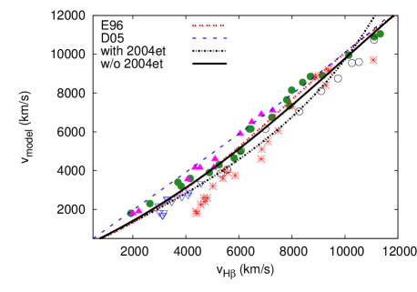
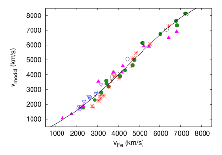
Figure 8: (a) The plot of $v_{model}$ against $v_{H\beta}$. The lines represent the polynomials calculated by Jones et al. (2009) (see text) based on the models of E96 (red dotted line), D05 (blue dashed line). The result from our fitting on all SNe is plotted as a black dotted line line while the fitting omitting SN 2004et is shown by a black solid line. (b) The same fitting as (a) but for $v_{Fe}$ using all SNe. The simbols have the same meaning as in Fig.4. The polynomial coefficients are in Table 2.

5.1 Velocity-velocity relations

Using the synthetic spectra of E96 and D05, Jones et al. (2009) also examined the relation between $v_{H\beta}$ and $v_{model}$. They found that their ratio can be described as

$${v_{H\beta}\over v_{model}}=\sum_{j=0}^{2}a_{j}v_{H\beta}^{j}$$ (1)

where the values of $a_{j}$ are given in Table 2. In Fig. 8 we plotted our data together with these polynomials. The polynomials based on the D05 models overestimate our $v_{model}$ values (rms $\sigma=0.412$), while those from the E96 models provide much better fit for all SNe except SN 2004et (rms $\sigma=0.301$, but $\sigma=0.178$ without the data of SN 2004et).

We fitted Eq.(1) to our data (Fig. 8, black curve). The resulting $a_{j}$ coefficients are in Table 2. Our fit resulted in a much lower rms scatter, $\sigma=0.276$. Repeating the fitting while omitting the data of SN 2004et, the result became very similar to that from the E96 models.

Since $v_{Fe}$ is thought to be a better representative of the velocity at the photosphere than $v_{H\beta}$, it is expected that $v_{model}$ can be predicted with better accuracy by measuring $v_{Fe}$. Indeed, Fig. 7 suggests that the $v_{Fe}/v_{model}$ ratio is almost the same from SN to SN, unlike the $v_{H\beta}/v_{model}$ ratio that can be quite different for different SNe. Thus, we repeated the fitting of Eq.(1) using $v_{Fe}$ instead of $v_{H\beta}$ (Fig. 8). We found the rms scatter of $\sigma=0.111$, which is much lower than in the previous cases. The $a_{j}$ coefficients of this fitting are also included in Table 2.

The tight relation between $v_{Fe}$ and $v_{model}$ in Fig. 8 suggests a possibility to estimate $v_{model}$ from the measured $v_{Fe}$ values. However, it is emphasized that SN-specific differences in the expansion velocities may exist, thus, model building for a particular SN, whenever possible, should always be preferred.

Nugent et al. (2006) found that $v_{Fe}$ evolves as

$$v_{Fe}(t)/v_{Fe}(50\mathrm{d})=(t/50)^{c}$$ (2)

where $c=-0.464\pm 0.017$. After repeating the fitting of Eq.(2) to our data, we found the exponent to be $c=-0.663\pm 0.01$. Then, since the data of SN 2005cs are very different from the rest of the sample, we omitted the velocities of SN 2005cs and repeated the fitting. This resulted in $c=-0.546\pm 0.01$ (Fig. 9). These two exponents marginally differ (at $\sim 1\sigma$) from the value given by Nugent et al. (2006). A possible source of this difference (beside the different velocity measurement techniques applied) may be that our sample covers the phases between +13 and +104 days, while the data by Nugent et al. (2006) are between +9 and +75 days.

We also examined how the SYNOW model velocities evolve in time. Combining Eq.(1) and Eq.(2), the following relation has be derived (again, excluding SN 2005cs from the sample):

$$v_{model}(t)/v_{model}(50\mathrm{d})={(t/50)^{-0.210\pm 0.11}\over\sum_{j=0}^{2}b_{j}(t/50)^{j}}$$ (3)

where $b_{0}=0.467\pm 0.15$, $b_{1}=0.327\pm 0.23$ and $b_{2}=0.174\pm 0.11$. The rms scatter is $\sigma=0.148$ (Fig. 9).

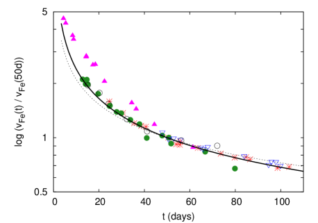
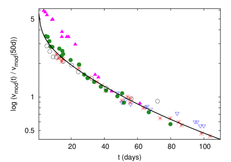
Figure 9: (a) The evolution of $v_{Fe}(t)/v_{Fe}(50\mathrm{d})$ and (b) the same for $v_{model}(t)/v_{model}(50\mathrm{d})$. The dashed line is the result by Nugent et al. (2006), while the solid lines are from our fittings (see text). The data of SN 2005cs (filled triangles) were excluded from the fitting. The color codes are the same as in Fig. 7.

Table 2: Polynomial coefficients for the $v_{H\beta}$ and $v_{Fe}$ to $v_{model}$ ratio (Eq.1).

j	0	1	2	$\sigma$	ref.
$a_{j}$ ($H_{\beta}$) (E96)	1.775	-1.435e-4	6.523e-9	0.30	(1)
$a_{j}$ ($H_{\beta}$) (D05)	1.014	4.764e-6	-7.015e-10	0.41	(1)
$a_{j}$ ($H_{\beta}$)	1.528	-1.551e-5	-3.462e-9	0.27	(2)
$a_{j}$ ($H_{\beta}$) w/o 04et	1.578	-8.573e-5	3.017e-9	0.17	(2)
$a_{j}$ (Fe ii $\lambda 5169$)	1.641	-2.297e-4	1.751e-8	0.11	(2)

• (1) Jones et al. (2009)

• (2) this paper

As was mentioned in §3.1, using SDSS data Poznanski et al. (2010) examined the correlation between velocities measured from the absorption minima of H$\beta$ and Fe ii $\lambda 5169$ lines (see Fig. 10). They found that there is a linear relation given by $v_{Fe}(50\mathrm{d})=a\cdot v_{H\beta}(50\mathrm{d})$, where $a=0.84\pm 0.05$. Using our sample we repeated their fitting. First, we used all epochs where both $v_{H\beta}$ and $v_{Fe}$ were measured. The slope of the fitted line was $a=0.791\pm 0.012$ ($\sigma=0.146$). Then, we kept only the velocities obtained before day 40 (similar to Poznanski et al., 2010). This resulted in $a=0.823\pm 0.015$ ($\sigma=0.102$), which is basically the same as that of Poznanski et al. (2010). Thus, our study fully confirms the results by Poznanski et al. (2010), but extends the validity of the relation toward later phases.

Figure 10: The relation between the measured $v_{Fe}$ and $v_{H\beta}$ values. The empty circles show the data taken after day 40, while the filled circles refer to data taken before day 40. The line shows the fit to the filled circles only.

6 Implications for distance measurements

Improving the accuracy of the velocity measurements has an important aspect in measuring extragalactic distances with SCM or EPM (cf. §1). Both SCM and EPM need velocities, thus, the results of this paper can be significant for both techniques.

SCM was calibrated using $v_{Fe}$ on day +50. However, in many cases getting a spectrum at or around day +50 is not possible. In these cases Eq.(2) can be used to estimate $v_{Fe}(50\mathrm{d})$. We have improved the exponent in Eq.(2) as $-0.546\pm 0.01$, based on more data obtained on wider range of phase than previously. The difference between our result and the previous curve (Nugent et al., 2006) is the highest around day +20 (Fig.9). The new curve may result in better constrained $v_{Fe}(50\mathrm{d})$ when only early-phase spectra obtained around day +20 are available.

However, there are several drawbacks of SCM. For example, the uncertainty in the moment of explosion, i.e. in determining the phase of a particular spectrum can lead to significant error in the distance determination. Moreover, as the example of SN 2005cs shows in Fig.9, some Type II-P SNe can deviate significantly from the average, especially during early phases. Thus, one should be careful when such kind of interpolation or extrapolation is to be applied. The example of SN 2005cs suggests that multi-epoch spectroscopic observations should always be preferred against single-epoch spectra when distance determination is the aim.

The case of EPM is different. Since this method does not require calibration, but needs multi-epoch data, deviations in the measured velocities have higher impact. To show this, we calculated the EPM–distances of all 5 SNe via the method described in Vinkó et al. (2011). We used two sets of velocities for each SNe: $i)$ from the absorption minimum of the Fe $\lambda$5169 line, $ii)$ $v_{model}$ determined in Sec. 3.4.

The resulted distances are in Table 3. The correction factors of D05 were applied for all SNe. Usually the photometric data were interpolated to the epochs of the velocities. However, for SN 2004dj Eq. 2 and Eq. 3 were used to extrapolate the velocity data to the photometric epochs, because of the low number of spectra taken before day +50, i.e. during the expansion of the photosphere.

6.1 SN 1999em

Data on SN 1999em in NGC 1637 were used for distance determination with EPM several times. Hamuy et al. (2001) used cross-correlation velocities (with the model spectra of E96 as the template set) and the correction factors of E96 to obtain the distance of $7.8\pm 0.5$ Mpc. Using absorption minima velocities and the same correction factors, Leonard et al. (2002) determined the distance as $8.2\pm 0.6$ Mpc, while Elmhamdi et al. (2003) obtained $7.8\pm 0.3$ Mpc. On the other hand, Leonard et al. (2003) determined the distance of NGC 1637 using Cepheids as $11.7\pm 1$ Mpc, which is significantly higher. Using the SEAM method, Baron et al. (2004) got $12.5\pm 1.8$ Mpc. With the velocities of their CMFGEN models and and the correction factors of D05, Dessart & Hillier (2006) derived $11.5\pm 1$ Mpc, and with a similar approach to that of Baron et al. (2004) they obtained $12.2\pm 2$ Mpc. Recently Jones et al. (2009) estimated the photospheric velocity from $v_{H\beta}$ (§5.1 Eq. 1), and derived $9.3\pm 0.5$ Mpc by using the correction factors of E96, and $13.9\pm 1.4$ Mpc from the correction factors of D05.

We have repeated the EPM analysis using D05 correction factors and our $v_{model}$ velocities. This resulted in $12.5\pm 1.4$ Mpc, which is in good agreement with the cepheid- and SEAM-distances and that of Dessart & Hillier (2006) using the velocities determined from their CMFGEN models. Instead, applying the $v_{Fe}$ velocities (extrapolating for the first few points using Eq.2), the distance became lower, $9.7\pm 0.8$ Mpc. The disagreement between these two distances is roughly the same as that due to the application of different correction factors (see above). The distance obtained from adopting the $v_{model}$ velocities is in much better agreement with the independent Cepheid-based distance to the host galaxy. It suggests that the application of the proper velocity data is important to obtain more realistic and bias-free distances from Type II-P SNe.

6.2 SN 2004dj

There are many published distances for the host galaxy of SN 2004dj (NGC 2403), but they show large scatter, being between $2.88$ and $6.43$ Mpc, according to the NED database.

In the case of this SN the velocity curve was extrapolated using Eq. 2 and Eq. 3 to the epochs of the photometry of Vinkó et al. (2006) and Tsvetkov et al. (2008). The distances from the two velocity curves agree very well ($D=3.6\pm 0.6$ and $3.7\pm 0.8$ Mpc, respectively, Table 3), and they are also in very good agreement with the result of Vinkó et al. (2006).

6.3 SN 2004et

Similarly, the distances of NGC 6946, the host galaxy of SN 2004et, show large scatter being in the range of $4.7$ and $7.2$ Mpc (NED). $D\sim 4.7$ Mpc was derived recently by Poznanski et al. (2009) using SCM.

Our result supports this shorter value. The EPM-analysis with both $v_{model}$ and $v_{Fe}$ (after extrapolation to the early phases by Eq. 2) gave $4.8$ Mpc (Table 3).

6.4 SN 2005cs

In the case of SN 2005cs the application of $v_{model}$ resulted in a considerably longer distance ($8.6\pm 0.2$ Mpc) than the one using $v_{Fe}$ ($7.5\pm 0.2$ Mpc). This longer distance is in good agreement with a recent study by Vinkó et al. (2011), in preparation, who determined the distance of M51 via EPM by combining the data of SNe 2011dh and 2005cs, and obtained $8.4\pm 0.7$ Mpc. The reason for the slight difference between their result and ours with $v_{model}$ (although both papers used the same photometry, velocities and method) is that, unlike Vinkó et al. (2011), we did not fix the moment of explosion in EPM. Instead, we also optimized that parameter to keep consistency with the analysis of all the other objects in this paper.

6.5 SN 2006bp

For SN 2006bp and its host galaxy, NGC 3953, the distances are between $15.7$ and $21.0$ Mpc (NED). Both of our results fit into this wide range, but with the usage of $v_{model}$ we obtained slightly longer values ($20.7\pm 1.8$ Mpc) than with $v_{Fe}$ ($18.6\pm 1.5$ Mpc), the latter being closer to the distance of Dessart et al. (2008), i.e. $17.1$ and $17.5$ Mpc from SEAM and SCM, respectively.

Table 3: The EPM distances of the 5 SNe using different velocities.

SN	D (Mpc)		Photometry
	with $v_{model}$	with $v_{Fe}$
1999em	12.5 (1.4)	9.7 (0.8)	1,2,3
2004dj	3.6 (0.6)	3.7 (0.8)	4,5
2004et	4.8 (0.4)	4.8 (0.6)	6,7
2005cs	8.6 (0.2)	7.5 (0.2)	8
2006bp	20.7 (1.8)	18.6 (1.5)	9

• ¹ Source of photometry: (1) Hamuy et al. (2001), (2) Leonard et al. (2002), (3) Elmhamdi et al. (2003), (4) Vinkó et al. (2006), (5) Tsvetkov et al. (2008), (6) Maguire et al. (2010b), (6) Sahu et al. (2006), (8) Pastorello et al. (2009), (9) Dessart et al. (2008)

7 Conclusions

In this paper we investigated three methods for estimating photospheric velocities of Type II-P SNe. We focused on building model spectra with SYNOW, and compared the resulting $v_{model}$ velocities with those obtained by cross-correlation or simply measuring absorption minima of P Cygni features. Based on a sample of 81 spectra from 5 SNe, we showed that SYNOW provides very similar photospheric velocities to those derived by more sophisticated modeling codes, but in a faster, less computation-intensive way. This approach may be more extensively applicable, yet it preserves the advantages of using physically consistent model spectra to estimate parameters of SNe non-interactively, and without relying mostly on eye-ball estimates and human decisions.

We illustrated that the cross-correlation- and absorption minimum velocities, i.e. those determined by more conventional methods, suffer from phase-dependent systematic deviations from the model velocities. This has already been known from previous studies (e.g. Dessart & Hillier, 2005b), but we have extended the phase coverage of the modeled spectra, and revealed that such deviations become stronger below $v_{phot}\sim 3000$ km  s^-1, i.e. after day +60. At these late phases $v_{Fe}$ may overestimate $v_{model}$ by 30 - 50 % depending on the atmospheric properties of the particular SN.

Based on these results, we verified and updated the relations between the photospheric velocities and the ones estimated from the Doppler-shifts of the absorption minima of individual spectral lines. It was found that while the $v_{Fe}/v_{model}$ ratio appears to be nearly the same for all SNe studied here, it is not true for the velocities from the H$\beta$ line. We have derived a power-law relation to estimate $v_{model}$ from $v_{Fe}$ and/or $v_{H\beta}$, but due to the possibility of SN-dependent systematic deviations, we recommend the computation of parametrized models, whenever possible.

Using the model velocities, we re-determined the distances of the 5 SNe via EPM, and compared them with the ones calculated by using $v_{Fe}$. The distances obtained from $v_{model}$ are similar or slightly higher than those with $v_{Fe}$. For SN 1999em, which is the most thoroughly studied object in our sample, we were able to show that by using the model velocities the derived distance is more consistent with the Cepheid-based distance to the host galaxy. Although such a comparison was not possible for the other SNe due to the lack of reliable Cepheid distances, this result underlines the importance of the velocity measurement method in SN distance studies.

Despite its numerous advantages, EPM also suffers from caveats. One of them is the need for many photometric data and contemporaneous velocities (i.e. spectra) covering most of the plateau phase. This is hardly achievable for most SNe. A possible solution may be a careful interpolation between the measured data points. Previously, the weakest link was the poorly resolved velocity curve, thus, mainly the light curves were interpolated to the moments of velocity measurements (e.g. Hamuy, 2002). Based on our results in Sec. 4, the interpolation of the velocity curve to the epochs of photometric data via Eq.(3) may also be a possibility, resulting in a better sampled dataset for EPM. We intend to demonstrate the application of this approach for new SNe in a future paper (Takáts et al., in preparation).

Appendix A Early spectra of SN 2004et

Figure 11: Early spectra of SN 2004et

Soon after its discovery (Zwitter et al., 2004), six low-resolution optical spectra of SN 2004et were taken at the David Dunlap Observatory, Canada, with the Cassegrain spectrograph mounted on the 74” telescope. The spectra covered the 4000 - 8000 Å regime with a resolution of $\sim 800$ at 6000 Å(see the details on the data reduction in Vinkó et al., 2006). Due to the fixed North-South slit direction, the spectra could not be taken at the parallactic angle, thus, the slope of the continuum in the blue is affected by differential refraction. Table 4 contains the journal of these observations, and the spectra are plotted in Fig. 11.

Table 4: Journal of spectroscopic observations of SN 2004et

Date	JD-2,450,000	Phase(d)	Airmass	Observer
2004-10-03	3281.6	+11	1.2	JT, TK
2004-10-04	3282.8	+12	2.0	SM, JT
2004-10-05	3283.5	+13	1.1	HD, TK
2004-10-06	3284.9	+14	2.3	HD, JT
2004-10-07	3285.5	+15	1.1	HD, JT
2004-10-08	3286.9	+16	1.7	JT, JG

• ¹ Observers: JT: J. Thomson, TK: T. Koktay, SM: S. Mochnacki, HD: H. DeBond, JG: J. Grunhut

Appendix B SNe velocities measured with different techniques

In Table 5 we present the velocities obtained with SYNOW ($v_{model}$, see §3.4), along with those measured from the absorption minima of H$\beta$ and Fe ii $\lambda 5169$ ($v_{H\beta}$ and $v_{Fe}$), as well as those obtained with cross-correlation method using the observed spectra of SN 1999em as templates ($v_{cc\#1}$) and the CMFGEN models ($v_{cc\#2}$).

Table 5: The velocities (in km s^-1) obtained with different techniques: the photospheric velocities from the best-fitting SYNOW models ($v_{model}$), the Doppler-shift of the absorption minima of H$\beta$ and Fe ii $\lambda 5169$ features ($v_{H\beta}$ and $v_{Fe}$, respectively) and the cross-correlation velocities from templates consisting of the observed spectra of SN 1999em ($v_{cc\#1}$) and the CMFGEN models ($v_{cc\#2}$). The phase (in days) were calculated relative to the date in Table 1.

SN 1999em							SN 2004et
phase	$v_{model}$	$v_{H\beta}$	$v_{Fe}$	$v_{cc\#1}$	$v_{cc\#2}$		phase	$v_{model}$	$v_{H\beta}$	$v_{Fe}$	$v_{cc\#1}$	$v_{cc\#2}$
4.79	11050 (300)	11332	–		10341 (454)		11.10	9700 (450)	11072	–	9951 (153)	8781 (1316)
5.84	10900 (350)	11101	–		9858 (888)		12.30	8900 (250)	8878	–	8605 (86)	8470 (681)
6.84	9950 (250)	10141	–		9112 (878)		13.00	9100 (400)	9386	–	9724 (117)	8786 (1099)
7.64	8900 (200)	9148	–		8383 (832)		14.40	9200 (400)	9375	–	7617 (71)	8570 (482)
8.67	8850 (150)	8697	–		8544 (491)		15.00	8800 (100)	8894	–	8635 (64)	8545 (524)
12.84	8550 (500)	8406	7236		8513 (497)		16.40	8400 (400)	9282	–	9110 (73)	9060 (545)
14.14	7350 (500)	7913	6829		7575 (289)		24.60	7300 (550)	8018	6416	6624 (49)	–
14.67	8150 (350)	7992	7213		7708 (190)		30.60	6050 (300)	7487	5535	5779 (56)	–
15.14	7650 (150)	7802	6793		7380 (187)		35.50	5500 (200)	7091	4861	5112 (43)	5739 (350)
19.67	6750 (200)	7246	6019		6703 (242)		38.60	5100 (400)	6869	4695	4981 (45)	5513 (337)
24.66	6150 (300)	6393	5146		5779 (126)		40.70	4600 (600)	6842	4644	4943 (41)	5448 (256)
24.84	6150 (225)	6450	5172		5866 (194)		50.50	3750 (300)	5859	4040	4236 (49)	4252 (367)
27.84	5000 (200)	6060	4773		5446 (155)		54.00	4050 (200)	5468	3715	3727 (23)	4352 (244)
29.84	4650 (250)	5816	4693		5221 (201)		55.60	3600 (450)	5396	3686	3867 (37)	3895 (408)
33.84	4300 (100)	5251	4312		4394 (215)		55.76	3900 (250)	5578	3840	4048 (37)	4113 (228)
37.84	3900 (100)	4885	4083		4521 (159)		63.50	3200 (400)	5018	3539	3656 (43)	3678 (349)
41.04	3600 (200)	4164	3421		3691 (115)		73.60	2600 (450)	4674	3292	3327 (45)	3793 (217)
47.84	3200 (400)	3822	3528		3765 (163)		79.73	2600 (100)	4807	3133	3192 (31)	3504 (246)
50.74	3400 (150)	3699	3435		3661 (131)		84.79	2400 (200)	4725	3147	3172 (51)	3490 (257)
51.76	2800 (350)	–	3183		3147 (152)		86.50	2250 (200)	4561	3060	2876 (64)	3496 (148)
66.76	2300 (100)	2645	2869		3097 (146)		98.60	1900 (450)	4377	2740	2779 (22)	3268 (131)
79.84	1800 (400)	1928	2313		1634 (100)		103.7	1800 (150)	4412	2779	2708 (33)	3060 (201)
SN 2004dj							SN 2005cs
phase	$v_{model}$	$v_{H\beta}$	$v_{Fe}$	$v_{cc\#1}$	$v_{cc\#2}$		phase	$v_{model}$	$v_{H\beta}$	$v_{Fe}$	$v_{cc\#1}$	$v_{cc\#2}$
47.89	3350 (300)	4569	3183	3154 (40)	3471 (83)		3.44	7100 (200)	7275	–	17105 (1876)	30045 (365)
50.59	2750 (150)	4089	2920	2943 (63)	3401 (172)		4.41	6900 (150)	6848	6814	7703 (109)	7092 (705)
52.89	2900 (150)	4122	2949	3075 (75)	3243 (115)		5.39	6500 (250)	6487	6418	7594 (151)	6945 (586)
55.89	2650 (100)	3849	2897	2967 (72)	3124 (122)		8.43	5900 (300)	6050	5481	5745 (143)	5775 (71)
64.86	2500 (150)	3317	2625	2672 (45)	2887 (114)		8.84	5950 (100)	–	5222	5422 (209)	4337 (193)
65.85	2550 (100)	3282	2573	2678 (47)	2649 (106)		14.36	4150 (300)	5052	4167	4060 (52)	4119 (80)
67.86	2400 (150)	3468	2645	2700 (46)	2689 (118)		14.44	4600 (100)	5099	4213	3908 (43)	4591 (170)
83.89	2200 (200)	2967	2350	2384 (50)	2387 (114)		17.35	4150 (50)	4532	3763	3616 (49)	3757 (129)
94.67	1850 (250)	3010	2101	2222 (67)	2454 (145)		18.42	4150 (100)	4345	3788	3566 (58)	3742 (110)
95.87	1850 (200)	3178	2186	2302 (71)	2535 (161)		22.45	3550 (300)	4069	3049	3232 (51)	3765 (315)
97.87	1700 (150)	3132	2182	2270 (78)	2504 (156)		34.44	1900 (50)	2222	2318	2254 (19)	2505 (126)
99.86	1700 (150)	3118	2075	2208 (86)	2433 (153)		36.40	1800 (100)	2003	2142	2189 (38)	2202 (74)
							44.40	1350 (50)	–	1756	1907 (23)	2036 (182)
							61.40	1050 (50)	–	1311	1459 (24)	1611 (274)
SN 2006bp
phase	$v_{model}$	$v_{H\beta}$	$v_{Fe}$	$v_{cc\#1}$	$v_{cc\#2}$		phase	$v_{model}$	$v_{H\beta}$	$v_{Fe}$	$v_{cc\#1}$	$v_{cc\#2}$
5.30	12050 (400)	11251	–	11537 (138)	11131 (571)		24.26	7050 (200)	8278	6315	6573 (45)	7317 (329)
7.10	10750 (450)	11097	–	11407 (103)	10748 (875)		32.26	6150 (200)	6996	5199	5548 (28)	6308 (330)
9.10	9600 (200)	10526	–	10975(70)	10242 (657)		41.21	5050 (125)	6078	4445	4698 (46)	5281 (181)
11.11	9550 (450)	10265	–	8717 (69)	9941 (521)		56.19	4050 (200)	5562	3952	4022 (40)	4602 (180)
15.10	8750 (250)	9735	8013	8373 (67)	9176 (325)		72.04	3850 (150)	5313	3697	–	–
20.28	8100 (100)	9104	7267	7506 (79)	8147 (184)

Appendix C Parameters of the best-fitting SYNOW models

In Table 6 we present the parameters of the best-fitting SYNOW models, including: $\tau_{ref}$ of the main atoms/ions, the power-law exponent of the optical depth function ($n$), the photospheric temperature ($T_{bb}$) and photospheric velocity ($v_{phot}$) (see §3.4 for details).

Table 6: The SYNOW parameters of the best-fitting models of SN 1999em. The phases were calculated from the assumed moments of explosions listed in Table 1.

SN 1999em
phase	JD-2,451,000	$\tau_{ref}$										n	$T_{bb}$	$v_{phot}$
(days)	(days)	H i	He i	Na i	Si i	Si ii	Ca ii	Sc ii	Ti ii	Fe ii	Ba ii		(kK)	(km s-1)
4.79	481.79	2.80	0.25									3.0	14.2	11050
5.84	482.84	3.50	0.20									3.0	12.0	10900
6.84	483.84	4.90	0.40									3.0	11.0	9950
7.64	484.64	6.30	0.35									3.0	9.5	8900
8.67	485.67	7.30	0.20									3.5	13.6	8850
12.84	489.84	15.80	0.10									5.5	10.0	8550
14.14	491.14	21.10		0.20						0.30		5.0	11.0	7350
14.67	491.67	26.15	0.05	0.10			2.20			0.80	0.35	6.5	11.5	8150
15.14	492.14	20.20		0.10		0.25				0.70		4.5	10.4	7650
19.67	496.67	42.05		0.10			16.0	0.05	0.30	0.95	0.40	5.0	9.0	6750
24.66	501.66	113.50		0.55			131.9	0.25	2.10	1.85		8.0	8.3	6150
24.84	501.84	81.00		0.35			17.6	0.15	1.10	1.60	0.40	7.0	8.3	6150
27.84	504.84	73.95		0.40				0.30	1.80	2.25	0.20	6.0	8.2	5000
29.84	506.84	65.00		0.45				0.15	1.65	4.10		6.0	7.0	4650
33.84	510.84	42.20		1.10	0.01		95.0	0.05	1.20	2.20		4.5	5.2	4300
37.84	514.84	39.60		1.00	0.01	0.10		0.15	1.55	2.25		4.5	5.5	3900
41.04	518.04	57.20	0.20	1.70	0.01	0.35	458.0	0.20	4.05	4.25	0.20	7.0	6.8	3600
47.84	524.84	23.00		1.85	0.01	0.35	200.0	0.45	2.30	2.20	1.00	3.0	4.5	3200
50.74	527.74	30.80		2.05	0.01	0.35	90.0	0.65	3.75	3.35		4.5	5.3	3400
51.76	528.76	36.60		1.95	0.02		212.0	0.20	0.50	2.65	0.25	3.0	6.5	2800
66.76	543.76	16.80		5.65	0.03	0.40		1.25	7.45	6.45		3.5	5.5	2300
79.84	556.84	71.50		13.95	0.02	0.65	969.0	2.35	17.95	13.90	4.70	3.5	6.0	1800
SN 2004dj
phase	JD-2,450,000	$\tau_{ref}$										n	$T_{bb}$	$v_{phot}$
(days)	(days)	H i	He i	Na i	Si i	Si ii	Ca ii	Sc ii	Ti ii	Fe ii	Ba ii		(kK)	(km s-1)
47.89	3234.89	81.0		0.70		0.15		0.30	2.85	2.55	0.85	6.0	7.65	3350
50.59	3237.59	88.0		1.10	0.01			0.70	6.15	6.00	1.00	5.5	6.0	2750
52.89	3239.89	68.0		1.05	0.01	0.40		0.40	3.75	3.05	1.00	5.5	8.0	2900
55.89	3242.89	51.0		1.15	0.02	0.20		0.30	2.75	3.70	0.80	4.5	6.2	2650
64.86	3251.86	72.0		1.95	0.01	0.25		0.75	4.25	4.95	0.50	5.5	8.0	2500
65.85	3252.85	63.0		2.05	0.01	0.20		0.50	4.75	5.15	2.00	5.5	6.0	2550
67.86	3254.86	83.0		2.25	0.02	0.30		0.70	5.45	8.55	0.05	5.5	6.8	2400
83.89	3270.89	85.0		7.10	0.01	0.30		1.00	6.30	7.55	1.60	5.5	8.9	2200
94.67	3281.67	145.0		18.45	0.01	0.10		1.00	7.15	8.80	3.55	5.5	9.7	1850
95.87	3282.87	109.0		24.75	0.02	0.30		1.05	9.55	10.20	2.45	6.0	9.4	1850
97.87	3284.87	185.0		34.30	0.06	0.40		1.40	11.70	14.20	3.00	5.0	9.5	1700
99.86	3286.86	120.0		25.0				0.50	9.00	10.0	0.40	4.5	8.5	1700

• Source of spectra:

• ^a Leonard et al. (2002)

• ^b Hamuy et al. (2001)

Table 7: continued

for SN 2004et. SN 2004et phase JD-2,451,000 $\tau_{ref}$ n $T_{bb}$ $v_{phot}$ (days) (days) H i He i Na i Si i Si ii Ca ii Sc ii Ti ii Fe ii Ba ii (kK) (km s^-1) 11.10 281.60 3.75 0.20 4.5 80.0 9700 12.30 282.80 4.05 0.20 3.0 19.0 8900 13.00 283.50 6.40 0.20 5.0 52.0 9100 14.40 284.90 8.00 0.30 4.0 9.5 9200 15.00 285.50 7.25 0.15 5.0 43.0 8800 16.40 286.90 14.45 0.25 4.0 9.0 8400 24.60 295.10 10.0 0.10 4.00 0.85 0.20 3.0 11.0 7300 30.60 301.10 21.0 0.10 0.40 74.4 0.15 1.20 4.5 7.9 6050 35.50 306.00 41.0 0.10 0.05 97.0 0.85 2.15 0.05 5.5 7.4 5500 38.60 309.10 47.0 0.25 0.01 98.0 0.15 1.45 2.80 0.05 4.0 7.2 5100 40.70 311.20 36.0 0.15 0.05 95.8 0.25 0.75 2.05 0.30 3.5 6.8 4600 50.50 321.00 40.0 0.65 324.0 0.25 1.25 2.35 0.70 3.0 5.4 3750 54.00 324.50 81.7 0.90 0.01 0.75 32.7 0.55 4.60 3.55 6.0 7.6 4050 55.60 326.10 45.0 0.95 0.01 45.0 0.45 3.05 5.05 0.45 3.5 6.8 3600 55.76 326.26 58.8 1.20 0.02 25.0 0.20 2.90 2.50 4.0 7.3 3900 63.50 334.00 31.0 1.15 81.0 0.25 2.0 3.60 2.5 5.0 3200 73.60 344.10 79.0 2.30 100.0 0.60 2.75 5.05 1.10 3.0 4.8 2600 79.73 350.23 79.9 4.90 30.0 1.20 11.9 6.80 4.5 7.1 2600 84.79 355.29 142.0 7.35 0.01 0.50 10.0 0.65 9.15 5.45 3.5 6.2 2400 86.50 357.00 223.0 3.15 0.10 515.0 0.70 7.90 13.1 4.0 5.2 2250 98.60 369.10 72.25 6.05 50.0 0.80 3.10 4.70 1.10 2.5 4.5 1900 103.70 374.20 219.0 32.05 80.0 2.35 37.7 25.3 5.50 4.5 5.5 1800

• Source of spectra:

• ^a This paper.

• ^b Sahu et al. (2006)

• ^c Maguire et al. (2010b)

Table 8: continued

for SN 2005cs. (The second column is JD-2,453,000). SN 2005cs phase JD $\tau_{ref}$ n $T_{bb}$ $v_{phot}$ (days) (days) H i He i N ii Na i Mg i Si i Si ii Ca ii Sc ii Ti ii Fe ii Ba ii (kK) (km s${}^{-1})$ 3.44 552.44 3.90 0.30 0.10 4.0 15.0 7100 4.41 553.41 7.00 0.40 0.10 0.10 4.5 15.0 6900 5.39 554.39 10.6 0.30 0.10 5.5 13.6 6500 8.43 557.43 15.3 0.20 0.50 0.35 5.0 10.6 5900 8.84 557.84 9.00 0.30 0.60 0.45 9.5 9.8 5950 14.36 563.36 81.0 1.50 0.40 0.60 30.0 0.10 0.55 4.25 0.30 8.0 10.2 4150 14.44 563.44 49.0 1.00 0.25 0.35 0.50 27.0 0.20 0.90 1.30 0.35 7.0 9.8 4600 17.35 566.35 124.0 0.60 0.70 0.40 80.0 0.05 1.70 2.05 8.0 8.4 4150 18.42 567.42 168.0 0.90 0.50 0.70 5.00 0.50 1.40 1.50 8.5 9.6 4150 22.45 571.45 36.0 0.30 1.00 0.40 0.70 1.20 1.05 0.90 8.0 7.5 3550 34.44 583.44 52.0 5.10 0.40 0.30 800.0 2.30 6.90 9.0 4.0 5.0 6.5 1900 36.40 585.40 35.0 4.75 0.80 0.30 100.0 1.85 8.85 10.3 1.95 5.0 6.2 1800 44.40 593.40 23.0 23.9 0.01 0.35 200.0 4.75 25.45 24.1 7.85 5.0 6.2 1350 61.40 610.40 15.0 119.9 0.04 0.25 800.0 12.35 73.50 54.4 63.40 5.5 5.7 1050

Table 9: continued

for SN 2006bp SN 2006bp phase JD-2,451,000 $\tau_{ref}$ n $T_{bb}$ $v_{phot}$ (days) (days) H i He i N ii Na i Si ii Ca ii Sc ii Ti ii Fe ii Ba ii (kK) (km s^-1) 5.30 840.30 2.15 0.15 4.0 10.2 12050 7.10 842.10 3.20 0.15 3.5 12.0 10750 9.10 844.10 6.05 0.15 4.5 11.7 9600 11.11 846.11 10.35 0.20 5.5 12.7 9550 15.10 850.10 15.65 0.05 0.04 0.20 0.80 0.35 4.5 10.8 8750 20.28 855.28 26.70 0.03 0.20 0.40 23.0 0.08 0.20 1.30 4.5 9.5 8100 24.26 859.26 20.00 0.10 0.01 0.10 0.10 25.0 0.10 0.80 1.50 0.50 5.5 8.5 7050 32.26 867.26 59.70 1.50 0.55 129.0 0.30 1.65 1.75 0.20 6.0 8.0 6150 41.21 876.21 118.6 2.00 1.25 326.0 0.65 3.50 2.60 0.85 7.0 7.2 5050 56.19 891.19 145.1 1.00 4.65 300.0 0.20 6.40 5.35 0.20 6.0 7.2 4050 72.04 907.14 150.1 18.4 165.0 1.90 10.85 6.75 1.45 5.5 7.0 3850

References

- Baron et al. (2004) Baron, E., Nugent, P. E., Branch, D., Hauschildt, P. H., 2004, ApJ 616, L91
- Blondin & Tonry (2007) Blondin, S., Tonry, J. L., 2007, ApJ 666, 1024
- Branch et al. (2002) Branch, D. et al., 2002, ApJ 566, 1005
- Chugai et al. (2005) Chugai, N. N., Fabrika, S. N., Sholukhova, O. N., Goranskij, V. P., Abolmasov, P. K., Vlasyuk, V. V., 2005, AstL 31, 792
- Crockett et al. (2011) Crockett, R. M., Smartt, S. J., Pastorello, A., Eldridge, J. J., Stephens, A. W., Maund, J. R., Mattila, S., 2011, MNRAS 410, 2767
- D’Andrea et al. (2010) D’Andrea C. B., et al., 2010, ApJ, 708, 661
- D05 (2005a) Dessart, L., Hillier, D. J., 2005, A&A 437, 667
- Dessart & Hillier (2005b) Dessart, L., Hillier, D. J., 2005, A&A 439, 671
- Dessart & Hillier (2006) Dessart, L., Hillier, D. J., 2006, A&A 447, 691
- Dessart et al. (2008) Dessart, L. et al., 2008, ApJ 675, 644
- E96 (1996) Eastman, R. G., Schmidt, B. P., Kirshner, R., 1996, ApJ, 466, 911
- Eldridge et al. (2007) Eldridge, J. J., Mattila, S., Smartt, S. J., 2007, MNRAS 376, L52
- Elmhamdi et al. (2003) Elmhamdi, A. et al., 2003, MNRAS 338, 939
- Fisher (1999) Fisher, A., 1999, PhD thesis, University of Oklahoma
- Gaskell et al (1986) Gaskell, C. M., Cappellaro, E., Dinerstein, H. L., Garnett, D. R., Harkness, R. P., Wheeler, J. C., 1986, Apj, 306, L77
- Hamuy et al. (2001) Hamuy, M. et al., 2001, ApJ 558, 615
- Hamuy (2002) Hamuy, M., 2002, Ph.D thesis, The University of Arizona
- Hamuy et al. (2003) Hamuy, M., 2003, in Marcaide J.-M., Weiler K. W., eds., Proc. IAU Colloq. 192, Cosmic Explosions: On the 10th Anniversary of SN 1993J, Springer, Berlin, p. 535
- Hamuy & Pinto (2002) Hamuy, M., Pinto, P. A., 2002, ApJ 566, L63
- Hamuy et al. (2001) Hamuy, M. et al., 2001, ApJ 558, 615
- Hatano et al. (1999) Hatano, K., Branch, D., Fisher, A., Millard, J., Baron, E., 1999, ApJS 121, 233
- Immler et al. (2007) Immler, S. et al., 2007, ApJ 664, 435
- Jones et al. (2009) Jones, M. I. et al. 2009, ApJ 696, 1176
- Kasen et al. (2002) Kasen D., Branch D., Baron E., Jeffery D., 2002, ApJ, 565, 380
- Kirshner & Kwan (1974) Kirshner, R. P., Kwan, J., 1974 ApJ, 193, 27
- Kloehr (2005) Kloehr, W., Muendlein, R., Li, W., Yamaoka, H., Itagaki, K., 2005, IAU Circ. 8553, 1
- Kotak et al. (2005) Kotak, R., Meikle, P., van Dyk, S. D., Höflich, P. A., Mattila, S., 2005, ApJ 628, L123
- Leonard et al. (2002) Leonard, D. C. et al., 2002, PASP 114, 35
- Leonard et al. (2003) Leonard, D. C., Kanbur, S. M., Ngeow, C. C., Tanvir, N. R., 2003, ApJ 594, L247
- Li (1999) Li W. D., 1999, IAU Circ., 7294, 1
- Li et al. (2005) Li, W., Van Dyk, S. D., Filippenko, A. V., Cuillandre, J.-C., 2005, PASP, 117, 121
- Maguire et al. (2010a) Maguire, K., Kotak, R., Smartt, S. J., Pastorello, A., Hamuy, M., Bufano, F., 2010, MNRAS 403, L11
- Maguire et al. (2010b) Maguire, K. et al. 2010, MNRAS 404, 981
- Maíz-Apellániz et al. (2004) Maíz-Apellániz, J., Bond, H. E., Siegel, M. H., Lipkin, Y., Maoz, D., Ofek, E. O., Poznanski, D., 2004, ApJ 615, L113
- Maund et al. (2005) Maund, J. R., Smartt, S. J., Danziger, I. J. 2005, MNRAS 364, L33
- Misra et al. (2007) Misra, K., Pooley, D., Chandra, P., Bhattacharya, D., Ray, A. K., Sagar, R., Lewin, W. H. G., 2007, MNRAS 381, 280
- Nakano & Itagaki (2006) Nakano S., Itagaki K., 2006, IAU Circ. 8700, 4
- Nakano et al. (2004) Nakano, S., Itagaki, K., Bouma, R. J., Lehky, M., Hornoch, K., 2004, IAU Circ. 8377, 1
- Nugent et al. (2006) Nugent, P. et al. 2006, ApJ, 645, 841
- Pastorello et al. (2006) Pastorello, A. et al., 2006, MNRAS 370, 1752
- Pastorello et al. (2009) Pastorello, A. et al., 2009, MNRAS 394, 2266
- Poznanski et al. (2009) Poznanski, D., et al. 2009, ApJ 694, 1067
- Poznanski et al. (2010) Poznanski, D., Nugent, P. E., Filippenko, A. V., 2010, ApJ 721, 956
- Quimby et al. (2007) Quimby, R. M., Wheeler, J. C., Höflich, P., Akerlof, C. W., Brown, P. J., Rykoff, E. S., 2007, ApJ 666, 1093
- Roy et al. (2011) Roy, R. et al. 2011, MNRAS 414, 167
- Sahu et al. (2006) Sahu, D. K., Anupama, G. C., Srividya, S., Muneer, S., 2006, MNRAS 372, 1315
- Smartt (2009) Smartt, S. J., 2009, ARA&A 47, 63
- Smartt et al. (2002) Smartt, S. J., Gilmore, G. F., Tout, C. A., Hodgkin, S. T., 2002, ApJ 565, 1089
- Smartt et al. (2009) Smartt, S. J., Eldridge, J. J., Crockett, R. M., Maund, J. R., 2009, MNRAS 395, 1409
- Takáts & Vinkó (2006) Takáts, K., Vinkó, J., 2006, MNRAS 372, 1735
- Tsvetkov et al. (2008) Tsvetkov, D. Y., Goranskij, V., Pavlyuk, N., 2008, PZ 28, 8
- Thomas, Nugent, & Meza (2011) Thomas R. C., Nugent P. E., Meza J. C., 2011, PASP, 123, 237
- Utrobin (2007) Utrobin, V. P., 2007, A&A 461, 233
- Utrobin & Chugai (2008) Utrobin, V. P., Chugai, N. N., 2008, A&A 491, 507
- Utrobin & Chugai (2009) Utrobin, V. P., Chugai, N. N., 2009, A&A 506, 829
- Vinkó et al. (2006) Vinkó, J. et al., 2006, MNRAS, 369, 1780
- Vinkó et al. (2011) Vinkó, J. et al., 2011, in prep.
- Vinkó et al. (2009) Vinkó, J. et al., 2009, ApJ, 695, 619
- Wang et al. (2005) Wang, X., Yang, Y., Zhang, T., Ma, J., Zhou, X., Li, W., Lou, Y.-Q., Li, Z., 2005, ApJ 626, L89
- Zhang et al. (2006) Zhang, T., Wang, X., Li, W., Zhou, X., Ma, J., Jiang, Z., Chen, J., 2006, AJ 131, 2245
- Zwitter et al. (2004) Zwitter, T., Munari, U., Moretti, S., 2004, IAU Circ. 8413, 1