Analysis of a method to parameterize planar curves immersed in triangulations

Abstract

We prove that a planar $C^{2}$-regular boundary $\Gamma$ can always be parameterized with its closest point projection $\pi$ over a certain collection of edges $\Gamma_{h}$ in an ambient triangulation, by making simple assumptions on the background mesh. For $\Gamma_{h}$, we select the edges that have both vertices on one side of $\Gamma$ and belong to a triangle that has a vertex on the other side. By imposing restrictions on the size of triangles near the curve and by requesting that certain angles in the mesh be strictly acute, we prove that $\pi:\Gamma_{h}\rightarrow\Gamma$ is a homeomorphism, that it is $C^{1}$ on each edge in $\Gamma_{h}$ and provide bounds for the Jacobian of the parameterization. The assumptions on the background mesh are both easy to satisfy in practice and conveniently verified in computer implementations. The parameterization analyzed here was previously proposed by the authors and applied to the construction of high-order curved finite elements on a class of planar piecewise $C^{2}$-curves.

1 Introduction

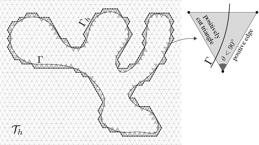
Fig. 1: Illustration of the choice of edges in an ambient triangulation used to parameterize a $C^{2}$-regular boundary. The curve $\Gamma$ is a cubic spline and is immersed in a nonconforming mesh of equilateral triangles. Triangles having one vertex inside the region enclosed by $\Gamma$ and two vertices outside are said to be positively cut and are shaded in gray. The edge of such a triangle joining its two vertices outside is called a positive edge; their union is denoted by $\Gamma_{h}$ and is drawn in dotted black lines. Theorem 5 identifies sufficient conditions for $\pi:\Gamma_{h}\rightarrow\Gamma$ to constitute a parameterization for $\Gamma$, where $\pi$ is its closest point projection. A critical one among these conditions is that a specific angle in each positively cut triangle be strictly acute, namely the one at the vertex of the positive edge closest to $\Gamma$, as illustrated in the triangle on the right.

The purpose of this article is to analyze a method to parameterize planar $C^{2}$-regular boundaries over a collection of edges in a background triangulation. Such a parameterization was introduced by the authors in [14]. The method consists in making specific choices for the edges in the background mesh and for the map from these edges onto the curve. For the edges, we select the ones that have both vertices on one side of the (orientable) curve to be parameterized and belong to a triangle that has a vertex on the other side, as illustrated in Fig. 1. Such edges are termed positive edges. For the map, we select the closest point projection of the curve. In this article, we prove that the closest point projection restricted to the collection of positive edges is a homeomorphism onto the curve and that it is $C^{1}$ on each positive edge (Theorem 5). For this, we have to impose restrictions on the size of a few triangles near the curve and request that certain angles in the background mesh be strictly smaller than $90^{\circ}$. We also compute bounds for the Jacobian of the resulting parameterization for the curve.

It is perhaps common knowledge that a sufficiently smooth curve can be parameterized with its closest point projection over the collection of interpolating edges in an adequately refined conforming triangulation. With Theorem 5, we generalize such an intuitive parameterization to also include nonconforming background meshes. In place of the interpolating edges in a conforming mesh, we pick the collection of positive edges in a nonconforming one, while still adopting the closest point projection to parameterize the curve. However, regularity for the curve and refinement for the mesh do not suffice. We also require certain angles in the mesh to be strictly acute, as depicted in Fig. 1. In practice, such an assumption is both easy to check and satisfy. It is perhaps surprising that a local algebraic condition on angles in triangles near the curve precipitates a global topological result. More so, because the angles required to be acute are irrelevant in the parameterization itself— neither the identification of positive edges nor the mapping onto the curve (the closest point projection) depend on them.

A compelling consequence of Theorem 5 is that any planar smooth boundary can be parameterized with its closest point projection over the collection of positive edges in any sufficiently refined background mesh of equilateral triangles. It is also interesting to note that the theorem does not guarantee the same with a background mesh of right-angled triangles. Such meshes may not satisfy the required assumption on angles, see (2b) in Theorem 5. On a related note, in [13, 14] we describe a way of parameterizing curves over edges and diagonals of meshes of parallelograms, which in particular includes structured meshes of rectangles. See also [3] for a triangulation algorithm with a similar objective.

The parameterization studied is independent of the particular description adopted for the curve, is easy to implement and readily parallelizable. It also extends naturally to planar curves with endpoints, corners, self-intersections, T-junctions and practically all planar curves of interest in engineering and computer graphics applications, see [14] and [13, Chapter 4]. The idea is to construct such curves by splicing arcs of $C^{2}$-regular boundaries and parameterize each arc with its closest point projection.

One of the main motivations behind the parameterization over positive edges is to accurately represent planar curved domains over nonconforming background meshes. For once the curved boundary is parameterized over a collection of nearby edges, we show in [13, Chapter 5] how a suitable collection of triangles in the background mesh can be mapped to curved ones to yield an exact spatial discretization for the curved domain. The construction of such mappings from straight triangles to curved ones and their analysis in the context of high-order finite elements with optimal convergence properties has been the subject of numerous articles; we refer to a representative few [4, 5, 7, 11, 12, 15, 16] for details on this subject. Almost without exception, these constructions have two assumptions in common: (i) a mesh with edges that interpolate the curved boundary and (ii) a (local) parametric representation for the curved boundary. The former entails careful mesh generation while the latter is a strong assumption on how the boundary is described. The parameterization analyzed here enables relaxing both these assumptions.

An outline of the proof of Theorem 5 is given in §3.3. The crux of the proof is demonstrating injectivity of the closest point projection $(\pi)$ over the collection of positive edges $(\Gamma_{h})$. Regularity of the parameterization and estimates for the Jacobian follow easily from regularity of the curve $(\Gamma)$ and some straightforward calculations. We prove injectivity by inspecting the restriction of $\pi$ to each positive edge, then to pairs of intersecting positive edges, and finally to connected components of $\Gamma_{h}$. That certain angles in the mesh be acute has a simple geometric motivation (see Fig. 2) and ensures injectivity over each positive edge (§A, §4). Extending this to the entire set $\Gamma_{h}$ is non-trivial, requiring some careful, albeit simple topological arguments. It entails understanding how and how many positive edges intersect at each vertex in $\Gamma_{h}$, leading us to show in §5 that each connected component of $\Gamma_{h}$ is a Jordan curve. We then show in §6 that the restriction of $\pi$ to each connected component of $\Gamma_{h}$ is a parameterization of a connected component of $\Gamma$. Finally in §7, we establish a correspondence between connected components of $\Gamma$ and $\Gamma_{h}$.

2 Preliminary definitions

In order to state our main result with the requisite assumptions, a few definitions are essential. First, we define the family of planar $C^{2}$-regular boundaries, the curves we consider for parameterization.

Definition 1 ([8, def. 1.2]).

A bounded open set $\Omega\subset{\mathbb{R}}^{2}$ has a $C^{2}$-regular boundary if there exists $\Psi\in C^{2}\left({\mathbb{R}}^{2},{\mathbb{R}}\right)$ such that $\Omega=\left\{x\in{\mathbb{R}}^{2}:\Psi(x)<0\right\}$ and $\Psi(x)=0$ implies $\left|\nabla\Psi\right|\geq 1$. We say that $\Omega$ is a $C^{2}$-regular domain and that $\partial\Omega$ is a $C^{2}$-regular boundary. The function $\Psi$ is called a defining function for $\Omega$.

There are a few equivalent notions of $C^{2}$-regular boundaries (and more generally $C^{k}$-regular boundaries), see [9]. For future reference, we note that each connected component of a $C^{2}$-regular boundary is a Jordan curve with bounded curvature.

We recall the definitions of the signed distance function and the closest point projection for a curve $\Gamma$ that is the boundary of an open and bounded set $\Omega$ in ${\mathbb{R}}^{2}$. The signed distance to $\Gamma$ is the map $\phi:{\mathbb{R}}^{2}\rightarrow{\mathbb{R}}$ defined as $-\min_{y\in\Gamma}d(\cdot,y)$ over $\Omega$ and as $\min_{y\in\Gamma}d(\cdot,y)$ elsewhere. The function $d(\cdot,\cdot)$ is the Euclidean distance in ${\mathbb{R}}^{2}$. The closest point projection $\pi$ onto $\Gamma$ is the map $\pi:{\mathbb{R}}^{2}\rightarrow\Gamma$ given by $\pi(\cdot)=\arg\min_{y\in\Gamma}d(\cdot,y)$.

The following theorem quoted from [8] is a vital result for our analysis. It concerns the regularity of the maps $\phi$ and $\pi$ for a $C^{2}$-regular boundary. The theorem also shows that $\phi$ is a defining function for a $C^{2}$-regular domain. In the statement, the $\varepsilon$-ball centered at $x\in{\mathbb{R}}^{2}$ is the set $B(x,\varepsilon):=\{y:d(x,y)<\varepsilon\}$ and the $\varepsilon$-neighborhood of $A\subset{\mathbb{R}}^{2}$ is the set $B(A,\varepsilon):=\cup_{x\in A}B(x,\varepsilon)$.

Theorem 2 ([8, Theorem 1.5]).

If $\Omega\subset{\mathbb{R}}^{2}$ is an open set with a $C^{2}$-regular boundary, then there exists $r_{n}>0$ such that $\phi:B(\partial\Omega,r_{n})\rightarrow(-r_{n},r_{n})$ and $\pi:B(\partial\Omega,r_{n})\rightarrow\partial\Omega$ are well defined. The map $\phi$ is $C^{2}$ while $\pi$ is a $C^{1}$ retraction onto $\partial\Omega$. The mapping $x\mapsto(\phi(x),\pi(x)):B(\partial\Omega,r_{n})\rightarrow(-r_{n},r_{n})\times\partial\Omega$ is a $C^{1}$-diffeomorphism with inverse $(\phi,\xi)\mapsto\xi+\phi\hat{N}(\xi):(-r_{n},r_{n})\times\partial\Omega\rightarrow B(\partial\Omega,r_{n})$ where $\hat{N}(\xi)$ is the unit outward normal to $\partial\Omega$ at $\xi$. Furthermore, $\phi$ is the unique solution of $|\nabla\phi|=1$ in $B(\partial\Omega,r_{n})$ with $\phi=0$ on $\partial\Omega$ and $\nabla\phi\cdot\hat{N}>0$ on $\partial\Omega$.

In Theorem 2, by saying that $\phi$ and $\pi$ are well defined over $B(\partial\Omega,r_{n})$, we mean that these maps are defined and have a unique value at each point in $B(\partial\Omega,r_{n})$. The following proposition follows from [6, §14.6]. A simple derivation specific to planar curves can be found in [14].

Proposition 3.

Let $\Gamma\subset{\mathbb{R}}^{2}$ be a $C^{2}$-regular boundary with signed distance function $\phi$, closest point projection $\pi$, signed curvature $\kappa_{s}$, and unit tangent $\hat{T}$. If $p\in B(\Gamma,r_{n})$ and $|\phi(p)\kappa_{s}(\pi(p))|<1$, then

$$\nabla\pi(p) =\frac{\hat{T}(\pi(p))\otimes\hat{T}(\pi(p))}{1-\phi(p)\,\kappa_{s}(\pi(p))},$$ (1a)

$$\text{and}\quad\nabla\nabla\phi(p) =-\kappa_{s}(\pi(p))\nabla\pi(p).$$ (1b)

For parameterizing $C^{2}$-regular boundaries, we will consider background meshes that are triangulations of polygonal domains (cf. [10, Chapter 4]). We mention the related terminology and notation used in the remainder of the article. With triangulation ${\cal T}_{h}$, we associate a pairing $(V,C)$ of a vertex list $V$ that is a finite set of points in ${\mathbb{R}}^{2}$ and a connectivity table $C$ that is a collection of ordered $3$-tuples in $V\times V\times V$ modulo permutations. A vertex in ${\cal T}_{h}$ is thus an element of $V$ (and hence a point in ${\mathbb{R}}^{2}$). An edge in ${\cal T}_{h}$ is a closed line segment joining two vertices of a member of $C$. The relative interior of an edge $e_{pq}$ with endpoints (or vertices) $p$ and $q$ is the set $\textbf{ri}\,(e_{pq})=e_{pq}\setminus\{p,q\}$.

A triangle $K$ in ${\cal T}_{h}$, denoted $K\in{\cal T}_{h}$, is the interior of the triangle in ${\mathbb{R}}^{2}$ with vertices given by its connectivity $\hat{K}\in C$. Frequently, we will not distinguish between $K$ and $\hat{K}$ unless the distinction is essential. We refer to the diameter of $K$ by $h_{K}$ and the diameter of the largest ball contained in $\overline{K}$ by $\rho_{K}$. The ratio $\sigma_{K}:=h_{K}/\rho_{K}$ is called the shape parameter of $K$ [10, Chapter 3]. Later, we will invoke the fact that $\sigma_{K}\geq\sqrt{3}$ with equality holding for equilateral triangles.

To consider curves immersed in background triangulations, we introduce the following terminology.

Definition 4.

Let $\Gamma\subset{\mathbb{R}}^{2}$ be a $C^{2}$-regular boundary with signed distance function $\phi$ and let ${\cal T}_{h}$ be a triangulation of a polygon in ${\mathbb{R}}^{2}$.

1. We say that $\Gamma$ is immersed in ${\cal T}_{h}$ if $\Gamma\subset\text{int}\left(\,\cup_{K\in{\cal T}_{h}}\,\overline{K}\,\right)$.

2. A triangle in ${\cal T}_{h}$ is positively cut by $\Gamma$ if $\phi\geq 0$ at precisely two of its vertices.

3. An edge in ${\cal T}_{h}$ is a positive edge if $\phi\geq 0$ at both of its vertices and if it is an edge of a triangle that is positively cut by $\Gamma$.

4. The proximal vertex of a triangle positively cut by $\Gamma$ is the vertex of its positive edge closest to $\Gamma$. When both vertices of the positive edge are equidistant from $\Gamma$, the one containing the smaller interior angle is designated to be the proximal vertex. If the angles are equal as well, either vertex of the positive edge can be assigned the proximal vertex.

5. The conditioning angle of a triangle positively cut by $\Gamma$ is the interior angle at its proximal vertex.

6. Let $K,K^{\text{adj}}\in{\cal T}_{h}$ be such that $K$ is positively cut by $\Gamma$, $K$ has positive edge $e$, $e\cap\Gamma\neq\emptyset$ and $\overline{K}\cap\overline{K^{\text{adj}}}=e$. Then, the angle adjacent to the positive edge of $K$, denoted $\vartheta_{K}^{\text{adj}}$, is defined as the minimum of the interior angles in $K^{\text{adj}}$ at the vertices of $e$.

3 Main result

The main result of this article is the following.

Theorem 5.

Consider a $C^{2}$-regular boundary $\Gamma\subset{\mathbb{R}}^{2}$ with signed distance function $\phi$, closest point projection $\pi$ and curvature $\kappa$. Let $\Gamma$ be immersed in a triangulation ${\cal T}_{h}$. Denote the union of positive edges in ${\cal T}_{h}$ by $\Gamma_{h}$ and the collection of triangles positively cut by $\Gamma$ in ${\cal T}_{h}$ by ${\cal P}_{h}$. For each $K\in{\cal P}_{h}$, let

$$\vartheta_{K} :=\text{conditioning angle of $K$},$$

$$\vartheta_{K}^{\text{adj}} :=\text{angle adjacent to positive edge of $K$ when defined},$$

$$M_{K} :=\max_{\overline{B(K,h_{K})}\cap\Gamma}\kappa\quad\text{and}\quad C_{K}^{h}:=\frac{M_{K}}{1-M_{K}h_{K}}.$$

Assume that for each connected component $\gamma$ of $\Gamma$, $\gamma_{h}:=\{x\in\Gamma_{h}\,:\,\pi(x)\in\gamma\}\neq\emptyset$. If for each $K\in{\cal P}_{h}$, we have

$$h_{K} <r_{n},$$ (2a)

$$\vartheta_{K} <90^{\circ}~{}\,$$ (2b)

$$0<\sigma_{K}C_{K}^{h}h_{K} <\min\left\{\cos\vartheta_{K},\sin\frac{\vartheta_{K}}{2}\right\},$$ (2c)

$$\text{and}\quad C_{K}^{h}h_{K} <\frac{1}{2}\sin\vartheta_{K}^{\text{adj}}\quad\text{whenever}~{}\vartheta_{K}^{\text{adj}}~{}\text{is defined,}$$ (2d)

then

1. each positive edge in $\Gamma_{h}$ is an edge of precisely one triangle in ${\cal P}_{h}$,

2. for each positive edge $e\subset\Gamma_{h}$, $\pi$ is a $C^{1}$-diffeomorphism over $\textbf{ri}\,(e\,)$,

3. if $K=(p,q,r)\in{\cal P}_{h}$ has positive edge $e_{pq}$, then

   $$- C_{K}^{h}h_{K}^{2}<\phi(x)\leq h_{K}\quad\forall x\in e_{pq}.$$ (3)

   The Jacobian $J$ of the map $\pi:\textbf{ri}\,(e_{pq})\rightarrow\Gamma$ satisfies

   $$0<\frac{\sin\left(\beta_{K}-\vartheta_{K}\right)}{1+M_{K}h_{K}}\leq J(x) =\left|\nabla\pi(x)\cdot\frac{(p-q)}{d(p,q)}\right|\leq\frac{1}{1-M_{K}h_{K}}\quad\forall x\in\textbf{ri}\,(e_{pq}),$$ (4)

   $$\text{where}\quad\cos\beta_{K} :=C_{K}^{h}\sigma_{K}h_{K}-\eta_{K},~{}\beta_{K}\in\left[0^{\circ},180^{\circ}\right],$$ (5)

   $$\eta_{K} :=\frac{\min\{\phi(p),\phi(q)\}-\phi(r)}{h_{K}}.$$ (6)

4. The map $\pi:\Gamma_{h}\rightarrow\Gamma$ is a homeomorphism. In particular, $\gamma_{h}$ as defined above is a simple, closed curve.

3.1 Discussion of the statement

With $\Gamma$ and $\Gamma_{h}$ as in the statement, Theorem 5 asserts sufficient conditions under which $\pi:\Gamma_{h}\rightarrow\Gamma$ is a homeomorphism. The statement of the theorem extends also to the case when edges in $\Gamma_{h}$ are identified using the function $-\phi$ instead of $\phi$. This corresponds to selecting the collection of negative edges for parameterizing $\Gamma$. Of course, a different collection of angles are required to be acute. If triangles in the vicinity of the curve are all acute angled, the theorem shows that there are two different collections of edges homeomorphic to $\Gamma$.

We make two important assumptions on the background mesh; we briefly examine them and discuss how they can be satisfied in practice in §3.2. The first assumption is, expectedly, on the size of triangles near $\Gamma$, as conveyed by conditions (2a), (2c) and (2d). For instance, if the mesh size is too large, then $\pi$ may not even be single valued over $\Gamma_{h}$.

Assumption (2b), which we term the acute conditioning angle assumption, is perhaps less intuitive. For once the set $\Gamma_{h}$ has been identified, the angles that positive edges make with other edges in the background mesh ${\cal T}_{h}$ are irrelevant. Rather, the rationale behind (2b) is that it provides a means to control the orientation of positive edges with respect to local normals to the curve. We explain this idea below using a simple example.

It is worth emphasizing that the assumptions on the background mesh in (2) are not very restrictive principally because there is no conformity required with $\Gamma$. Besides, the region triangulated by ${\cal T}_{h}$ can be quite arbitrary and need only contain $\Gamma$ in the sense of definition 4(i). In particular, while considering ambient triangulations of larger sets, the restrictions on the size, quality and angles stemming from (2) apply only to a subset of the collection of triangles intersected by $\Gamma$, namely positively cut triangles and triangles having positive edges that are intersected by $\Gamma$.

Finally, we mention that Theorem 5 guarantees a parameterization for $\Gamma$ provided the collection of triangles positively cut by each of its connected components is non-empty. This is apparent from the fact that all restrictions on the mesh size and angles in (2) apply only to positively cut triangles and triangles having positive edges that are intersected by $\Gamma$. For instance, if a connected component $\gamma$ of $\Gamma$ is a contained in the interior of a triangle in ${\cal T}_{h}$, then no triangle is positively cut by it. Of course, it is possible for the collection of triangles positively cut by $\gamma$ to be empty in a multitude of ways. In principle, sufficient conditions are easily identified to ensure at least one triangle is positively cut by each connected component of $\Gamma$. In practice however, it is much simpler to inspect the sign of $\phi$ at the vertices of triangles and verify the presence of positively cut triangles rather than check such conditions.

3.1.1 The acute conditioning angle assumption

Fig. 2: Illustration to explain the rationale behind the acute conditioning angle assumption. Triangle $K$ is positively cut by $\Gamma$. Although $\beta_{K}>90^{\circ}$, it can be arbitrarily close to $90^{\circ}$ by changing the locations of vertices $b$ and $c$. Requesting $\vartheta_{K}<90^{\circ}$ ensures that $\beta_{K}-\vartheta_{K}>0^{\circ}$ always and hence that $\pi(e_{ab})$ has non-zero length.

Consider a locally straight curve $\Gamma$ as shown in Fig. 2. Triangle $K$ shown in the figure is positively cut by $\Gamma$, has positive edge $e_{ab}$ and proximal vertex $a$. Abusing the definition in (5), we have $\cos\beta_{K}=-\eta_{K}h_{K}/d(a,c)$ as indicated in the figure (the two definitions coincide if the length of the edge $e_{ac}$ is $h_{K}$). The projection of $e_{ab}$ onto $\Gamma$ has length $d(a,b)\sin(\beta_{K}-\vartheta_{K})$. For $\pi$ to be injective over $e_{ab}$, we need to ensure that $0^{\circ}<\beta_{K}-\vartheta_{K}<180^{\circ}$. Even though the angle $\beta_{K}$ depicted in the figure is strictly larger than $90^{\circ}$, it can be made arbitrarily close to $90^{\circ}$ by altering the locations of vertices $a$ and $c$. Therefore, we request that the conditioning angle $\vartheta_{K}$ be smaller than $90^{\circ}$ thereby ensuring $\beta_{K}-\vartheta_{K}>0^{\circ}$. The assumptions $\phi(a)\leq\phi(b)$ and $\vartheta_{K}<90^{\circ}$ together imply that $\beta_{K}-\vartheta_{K}<180^{\circ}$.

We refer to [13, 14] for simple examples where $\pi$ fails to be injective over $\Gamma_{h}$ because the conditioning angle fails to be acute. Of course, (2b) is only a sufficient condition for injectivity. In fact, a simple way to relax assumption (2b) is by defining an equivalence relation $\stackrel{{\scriptstyle\Gamma}}{{\simeq}}$ over the family of triangulations in which $\Gamma$ is immersed. Consider two triangulations ${\cal T}_{h}=(V,C)$ and ${\cal T}^{\prime}_{h^{\prime}}=(V^{\prime},C^{\prime})$. We say ${\cal T}_{h}\stackrel{{\scriptstyle\Gamma}}{{\simeq}}{\cal T}^{\prime}_{h^{\prime}}$ if there is a bijection $\Phi:V\rightarrow V^{\prime}$ such that

1. $(p,q,r)\in C\iff(\Phi(p),\Phi(q),\Phi(r))\in C^{\prime}$,

2. $\phi(v)\geq 0\iff\phi(\Phi(v))\geq 0$,

3. $\phi(v)<0\iff\phi(\Phi(v))<0$,

4. $v\in\Gamma_{h}\Rightarrow\Phi(v)=v$.

The map $\Phi$ can be interpreted as a (constrained) perturbation of vertices in ${\cal T}_{h}$ to yield a new mesh ${\cal T}^{\prime}_{h^{\prime}}$. It is clear from the definition of the equivalence relation that both ${\cal T}_{h}$ and ${\cal T}^{\prime}_{h^{\prime}}$ have exactly the same set of positive edges even though their positively cut triangles can have very different conditioning angles. The key point is that the result of the theorem can be applied to ${\cal T}_{h}$ from merely knowing the existence of a triangulation in its equivalence class that has acute conditioning angle. In light of this observation, the theorem applies even to some families of background meshes that do not satisfy assumption (2b).

With no conformity requirements on the background mesh, the acute conditioning angle assumption (2b) is easy to satisfy in practice. A simple way for example, is to ensure that triangles in the vicinity of $\Gamma_{h}$ in the background mesh are acute angled; even simpler— use background meshes consisting of all acute angled triangles. Such acute triangulations, including adaptively refined ones, are conveniently constructed by tiling quadtrees using stencils of acute angled triangles provided in [2].

3.2 Restrictions on triangle sizes

Conditions restricting the mesh size, namely (2a), (2c) and (2d), were identified by simply tracking the restrictions on the mesh size in the proof of Theorem 5. They are easily checked for a given curve and background mesh and can be used to guide refinement of background meshes near the boundaries of domains. Furthermore, they make transparent what parameters related to the curve and to the mesh influence how much refinement is required. For instance, (2a) shows that a more refined mesh is required if the curve has small features. The requirement that $\sigma_{K}C_{K}^{h}h_{K}$ be positive in (2c) is equivalent to $M_{K}h_{K}<1$, which reveals that smaller triangles are required where the curve has large curvature. More refinement is also needed when conditioning angles are close to $90^{\circ}$, when triangles are poorly shaped as indicated by large values of $\sigma_{K}$ or small values of $\vartheta_{K}^{\text{adj}}$.

Commonly used meshing algorithms usually guarantee shape regularity and bounds for interior angles in triangles with mesh refinement. Consequently, there exist mesh size independent constants $\sigma>0$ and $0^{\circ}<\theta_{\text{min}}\leq\theta_{\text{max}}<180^{\circ}$ such that the shape parameter is bounded by $\sigma$ and interior angles of triangles are bounded between $\theta_{\text{min}}$ and $\theta_{\text{max}}$. As discussed above, conditioning angles can be guaranteed to be acute independent of the mesh size. For example, $\vartheta_{K}=60^{\circ}$ for background meshes of equilateral triangles. Angles in triangulations constructed using stencils in [2] are guaranteed to lie between $36^{\circ}$ and $80^{\circ}$.

It is imperative also to consider if the requirements on the mesh size posed by (2) are too conservative. We check this for a specific example of a circle of radius $R$ immersed in a background mesh of equilateral triangles. In such a case, we have $h_{K}=h$ for each triangle in the mesh, and $\vartheta_{K}=60^{\circ},\sigma_{K}=\sqrt{3},r_{n}=M_{K}=1/R$ and $\vartheta_{K}^{\text{adj}}=60^{\circ}$ (when defined) for each positively cut triangle $K$. Then, satisfying (2) requires $h<h_{0}:=R/(1+2\sqrt{3})\simeq 0.224R$. The a priori estimate $h_{0}=0.224R$ is a reasonable one because it is comparable to $R$. Of course, the estimate will change with the choice of background meshes.

3.2.1 Bound for the Jacobian

Eq.(4) provides an estimate for the Jacobian of the parameterization. Inspecting the lower bound in (4), which is the critical one, shows that $J\geq\sin(\beta_{K}-\vartheta_{K})$ if $M_{K}h_{K}=0$. This is precisely the Jacobian computed for a line, as in figure 2, when the definitions of $\beta_{K}$ in (5) is replaced by that in the figure. The same interpretation of the lower bound holds when $M_{K}\not=0$ but $h_{K}$ is small. In this case, each positive edge parameterizes a small subset of $\Gamma$, which appears essentially straight.

For reasonably large values of $M_{K}h_{K}$, the angle $\beta_{K}$ in (5) can be close to $90^{\circ}$, even acute. Hence $\beta_{K}-\vartheta_{K}$ can be small. In light of this, we mention that a smaller conditioning angle yields a better parameterization, one with $J$ closer to $1$. Finally, with mesh size independent bounds for $\sigma_{K}$ and $\vartheta_{K}$, it is straightforward to demonstrate that the estimates for $J$ in (4) are in turn bounded away from zero independent of the mesh size (specifically, $\beta_{K}-\vartheta_{K}$ and $1\pm M_{K}h_{K}$ appearing in the estimate can be bounded independent of the mesh size).

3.3 Outline of proof

We briefly discuss the outline of the proof of Theorem 5. The critical step is showing that $\pi$ is injective over $\Gamma_{h}$. To this end, we proceed in simple steps by considering the restriction of $\pi$ over each positive edge, then over pairs of intersecting positive edges and finally over connected components of $\Gamma_{h}$.

In Appendix A, we compute bounds for the signed distance function $\phi$ on $\Gamma_{h}$ and for angles between positive edges and local tangents/normals to $\Gamma$. By requiring that size of positively cut triangles be sufficiently small and by invoking assumption (2b), we show that a positive edge is never parallel to a local normal to $\Gamma$ (Proposition 7). From here, we infer that $\pi$ is injective over each positive edge (Lemma 8). The required bounds for the Jacobian in (4) also follow easily from the angle estimates. Part (ii) of the theorem is then a direct consequence of the inverse function theorem.

A logical next step is to show that $\pi$ is injective over each pair of intersecting positive edges (Proposition 16). For this, in §5 we first examine how positive edges intersect. Lemma 13 states that precisely two positive edges intersect at each vertex in $\Gamma_{h}$. This result leads us to conclude that $\Gamma_{h}$ is in fact a collection of simple, closed curves (Lemma 14).

Knowing that (i) $\pi$ is injective over each pair of intersecting positive edges, (ii) each connected component of $\Gamma_{h}$ is a simple, closed curve and (iii) $\pi$ is continuous over $\Gamma_{h}$, we demonstrate (in Lemma 15) that $\pi$ is a homeomorphism over each connected component of $\Gamma_{h}$. What remains to be shown is that precisely one connected component of $\Gamma_{h}$ is mapped to each connected component of $\Gamma$. We do this in §7 by illustrating that the collection of positive edges that map to a connected component of $\Gamma$ is itself a connected set (Lemma 19).

3.4 Assumptions and notation for subsequent sections

In all results stated in subsequent sections, we presume that the (2) in the statement of Theorem 5 hold. In several intermediate results, one or more of these assumptions could be relaxed.

We shall denote the unit normal and unit tangent to $\Gamma$ at $\xi\in\Gamma$ by $\hat{N}(\xi)$ and $\hat{T}(\xi)$ respectively. We assume an orientation for $\Gamma$ such that $\hat{N}=\nabla\phi$ on the curve, and that $\{\hat{T},\hat{N}\}$ constitutes a right-handed basis for ${\mathbb{R}}^{2}$ at any point on the curve. Given distinct points $a,b\in{\mathbb{R}}^{2}$, we denote the unit vector pointing from $a$ to $b$ by $\hat{U}_{ab}$ and define $\hat{U}_{ab}^{\perp}$ such that $\{\hat{U}_{ab},\hat{U}_{ab}^{\perp}\}$ is a right-handed basis.

The following simple calculation establishes the ranges of parameters $\eta_{K}$ and $\beta_{K}$ introduced in the statement of Theorem 5. Furthermore, for each $K\in{\cal P}_{h}$, part (ii) of Proposition 6 together with (2a) implies that $\overline{K}\subset B(\Gamma,r_{n})$. Then Theorem 2 shows that $\pi$ is $C^{1}$ and in particular, well defined over $\overline{K}$. Since any positive edge is an edge of some triangle in ${\cal P}_{h}$, we get that $\Gamma_{h}\subset B(\Gamma,r_{n})$ and hence that $\pi$ is well defined and continuous on $\Gamma_{h}$. We shall frequently use these consequences of the proposition in the remainder of the article, often without explicitly referring to it.

Proposition 6.

Let $K=(a,b,c)\in{\cal P}_{h}$. Then

1. $\overline{K}\cap\Gamma\neq\emptyset$. In particular, $\phi(c)<0\Rightarrow e_{bc}\cap\Gamma\neq\emptyset,e_{ac}\cap\Gamma\neq\emptyset$,

2. $|\phi|\leq h_{K}$ on $\overline{K}$,

3. $\eta_{K}$ defined in (6) satisfies $0<\eta_{K}\leq 1$,

4. $\beta_{K}$ given by (5) is well defined and $\beta_{K}>\vartheta_{K}$.

Proof.

We only show (iv) and the upper bound in (iii), since the others follow directly from the definitions. To this end, assume that $\phi(c)<0$ and $\phi(a),\phi(b)\geq 0$, and consider any $\xi\in e_{ac}\cap\Gamma$. From the definition of $\eta_{K}$ in (6), we have

$$\eta_{K}h_{K}\leq\phi(a)-\phi(c)\leq d(a,\Gamma)+d(c,\Gamma)\leq d(a,\xi)+d(c,\xi)\leq h_{K},$$

which shows that $\eta_{K}\leq 1$. To show that $\beta_{K}$ is well defined, we check that $\cos\beta_{K}\in[-1,1]$. Noting that $\sigma_{K}C_{K}^{h}h_{K}\geq 0$ and $\eta_{K}\leq 1$ shows that

$$\cos\beta_{K}=\sigma_{K}C_{K}^{h}h_{K}-\eta_{K}\geq-\eta_{K}\geq-1.$$

For the upper bound, we have

$$\cos\beta_{K} =\sigma_{K}C_{K}h_{K}-\eta_{K},$$

$$\leq\sigma_{K}C_{K}h_{K},\qquad~{}\left(\text{using}~{}\eta_{K}>0\right)$$

$$\leq\cos\vartheta_{K}\leq 1,\qquad\left(\text{from}~{}\eqref{eq:sigmaCh}\right)$$

which also shows that $\beta_{K}>\vartheta_{K}$. ∎

4 Injectivity on each positive edge

To show the injectivity of $\pi$ on each positive edge (Lemma 8) and estimate the Jacobian of this mapping (Lemma 11), we essentially follow the calculation illustrated in Fig. 2. In both arguments, we use the following angle estimate that is proved in Appendix A.

Proposition 7.

Let $K=(a,b,c)\in{\cal P}_{h}$ have positive edge $e_{ab}$ and proximal vertex $a$. Then

$$-\frac{3}{2}C_{K}^{h}h_{K} \leq\hat{N}(\pi(x))\cdot\hat{U}_{ab}\leq\cos(\beta_{K}-\vartheta_{K})\quad\forall x\in e_{ab}.$$ (7)

In particular, $|\hat{N}(\pi(x))\cdot\hat{U}_{ab}|<1$ and $|\hat{T}(\pi(x))\cdot\hat{U}_{ab}|>0$.

Lemma 8.

The restriction of $\pi$ to each positive edge in $\Gamma_{h}$ is injective.

Proof.

Let $(a,b,c)\in{\cal P}_{h}$ have positive edge $e_{ab}$ and proximal vertex $a$. We proceed by contradiction. Suppose that $x,y\in e_{ab}$ are distinct points such that $\pi(x)=\pi(y)$. From Theorem 2 and $\pi(x)=\pi(y)$, we have

$$x =\pi(x)+\phi(x)\hat{N}(\pi(x)),$$ (8a)

$$y =\pi(y)+\phi(y)\hat{N}(\pi(y))=\pi(x)+\phi(y)\hat{N}(\pi(x)).$$ (8b)

Noting $x\neq y$ in (8) implies that $\phi(x)\neq\phi(y)$. Therefore, subtracting (8b) from (8a) yields

$$\hat{N}(\pi(x)) =\frac{x-y}{\phi(x)-\phi(y)}.$$ (9)

By definition of $x,y\in e_{ab}$, $x-y$ is a vector parallel to $\hat{U}_{ab}$. Therefore (9) in fact shows that $|\hat{N}(\pi(x))\cdot\hat{U}_{ab}|=1$, contradicting Proposition 7. ∎

Before showing the bounds in (4) for the Jacobian, we prove Corollary 10, a useful step in showing part (iv) of Theorem 5. As discussed in §3.4, continuity of $\pi$ on each positive edge follows from part (ii) of Proposition 6. The continuity of its inverse is a consequence of Lemma 8 and the following result in basic topology, which we use here and later in §6.

Theorem 9 ([1, Chapter 3]).

A one-one, onto and continuous function from a compact space to a Hausdorff space is a homeomorphism.

Corollary 10 (of Lemma 8).

Let $e$ be a positive edge in $\Gamma_{h}$. Then $\pi:e\rightarrow\pi(e)$ is a homeomorphism.

Proof.

From part (ii) of Proposition 6 and Lemma 8, we know that $\pi$ is continuous and injective on $e$. The corollary then follows from Theorem 9. ∎

Lemma 11.

Let $K=(a,b,c)\in{\cal P}_{h}$ have positive edge $e_{ab}$. Then $\pi$ is $C^{1}$ over $\textbf{ri}\,(e_{ab})$ and

$$0<\frac{\sin\left(\beta_{K}-\vartheta_{K}\right)}{1+M_{K}h_{K}}\leq\left|\nabla\pi(x)\cdot\hat{U}_{ab}\right|\leq\frac{1}{1-M_{K}h_{K}}\leq\frac{5}{3}\quad\forall x\in e_{ab}.$$ (10)

Proof.

From part (ii) of Proposition 6 and (2a), we know $e_{ab}\subset B(\Gamma,r_{n})$. Then Theorem 2 shows that $\pi$ is $C^{1}$ over $\textbf{ri}\,(e_{ab})$.

Consider any $x\in\textbf{ri}\,(e_{ab})$. Since $|\phi(x)|\leq h_{K}$ (Proposition 6),

$$\kappa(\pi(x))\leq\max_{\overline{B(x,h_{K})}\cap\Gamma}\kappa\leq\max_{\overline{B(K,h_{K})}\cap\Gamma}\kappa=M_{K}.$$ (11)

Therefore, $|\phi(x)\kappa(\pi(x))|\leq M_{K}h_{K}$ which is smaller than $1$ because of the assumption $\sigma_{K}C_{K}^{h}h_{K}>0$ in (2c). Then from Proposition 1, we get

$$J(x) :=\left|\nabla\pi(x)\cdot\hat{U}_{ab}\right|=\frac{|\hat{U}_{ab}\cdot\hat{T}(\pi(x))|}{|1-\phi(x)\kappa_{s}(\pi(x))|},$$ (12)

where $\kappa_{s}$ is the signed curvature of $\Gamma$ (and $\kappa=|\kappa_{s}|$). From $|\phi(x)\kappa_{s}(\pi(x))|\leq M_{K}h_{K}<1$, we get

$$1-M_{K}h_{K}\leq|1-\phi(x)\kappa_{s}(\pi(x))|\leq 1+M_{K}h_{K}.$$ (13)

From Proposition 7, we have

$$\left|\sin(\beta_{K}-\vartheta_{K})\right|\leq\left|\hat{T}(\pi(x))\cdot\hat{U}_{ab}\right|\leq 1.$$ (14)

Note however from part (iv) of Proposition 6 that $\beta_{K}>\vartheta_{K}\Rightarrow\left|\sin(\beta_{K}-\vartheta_{K})\right|=\sin(\beta_{K}-\vartheta_{K})$. Then using (13) and (14) in (12) yields the lower and upper bounds for $|J(x)|$ in (10).

It remains to show that these bounds are meaningful, i.e., the lower bound is positive and the upper bound is not arbitrarily large. The former is a consequence of $\beta_{K}>\vartheta_{K}$ (from Proposition 6). We know from (2c) that $\sigma_{K}C_{K}^{h}h_{K}<\sin(\vartheta_{K}/2)<1$. Then, using $M_{K}h_{K}<1$ from (2c) and $\sigma_{K}\geq\sqrt{3}$, we get $M_{K}h_{K}<(1+\sqrt{3})^{-1}<2/5$, which renders the upper bound in (10) independent of $h_{K}$. ∎

By using the strictly positive lower bound for the Jacobian computed in the inverse function theorem, we conclude that $\pi:\textbf{ri}(e)\rightarrow\Gamma$ is a locally a $C^{1}$-diffeomorphism on each positive edge $e$. Since we have already shown the injectivity of this map in Lemma 8, part (ii) of Theorem 5 follows.

5 The set $\Gamma_{h}$

An essential step in showing that $\pi$ is injective over $\Gamma_{h}$ is understanding how positive edges intersect. The goal of this section is to demonstrate that $\Gamma_{h}$ is a union of simple, closed curves (Lemma 14). We achieve this by considering how many positive edges intersect at each vertex in $\Gamma_{h}$. In Lemma 13, we state that this number is precisely two. Additionally, as claimed in part (i) of Theorem 5 and stated below in Lemma 12, each positive edge belongs to precisely one positively cut triangle. The proofs of these two lemmas is somewhat laborious, and hence are included in Appendix B.

Lemma 12.

Each positive edge in ${\cal T}_{h}$ is a positive edge of precisely one triangle positively cut by $\Gamma$.

Lemma 13.

Precisely two distinct positive edges intersect at each vertex in $\Gamma_{h}$.

Lemma 14.

Let $\gamma_{h}$ be a connected component of $\Gamma_{h}$. Then $\gamma_{h}$ is a simple, closed curve that can be represented as as

$$\gamma_{h} =\bigcup_{i=0}^{n}e_{v_{i}v_{(i+1)\text{mod}\,(n)}},$$ (15)

where $v_{0},\ldots,v_{n}$ are all the distinct vertices in $\gamma_{h}$ and $2\leq n<\infty$.

Proof.

We will only prove (15). That $\gamma_{h}$ is a simple and closed curve follows immediately from such a representation.

Denote the number of vertices in $\gamma_{h}$ by $n+1$ for some integer $n$. Since $\gamma_{h}$ is non-empty, it contains at least one positive edge, say $e_{v_{0}v_{1}}$ with vertices $v_{0}$ and $v_{1}$. Lemma 13 shows that precisely two positive edges intersect at $v_{1}$. Therefore, we can find vertex $v_{2}\in\gamma_{h}$ different from $v_{0},v_{1}$ such that $e_{v_{1}v_{2}}$ a positive edge. This shows that $n\geq 2$. Of course $n<\infty$ because there are only finitely many vertices in ${\cal T}_{h}$.

We have identified vertices $v_{0},v_{1}$ and $v_{2}$ such that $e_{v_{0}v_{1}},e_{v_{1}v_{2}}\subset\gamma_{h}$. Suppose that we have identified vertices $v_{0},v_{1},\ldots,v_{k-1}$ for $k\in\{2,\ldots,n\}$ such that $e_{v_{i}v_{(i+1)}}\subset\gamma_{h}$ for each $0\leq i\leq k-2$. We show how to identify vertex $v_{k}$ such that $e_{v_{(k-1)}v_{k}}\subset\gamma_{h}$. Lemma 13 shows that precisely two positive edges intersect at $v_{(k-1)}$. One of them is $e_{v_{(k-2)}v_{(k-1)}}$. Let $v_{k}$ be such that $e_{v_{(k-1)}v_{k}}$ is the other positive edge. While $v_{k}$ is different from $v_{(k-2)}$ and $v_{(k-1)}$ by definition, it remains to be shown that $v_{k}\neq v_{i}$ for $0\leq i<k-2$. To this end, note that for $1\leq i<k-2$, we have already found two positive edges that intersect at $v_{i}$, namely $e_{v_{(i-1)}v_{i}}$ and $e_{v_{i}v_{(i+1)}}$. Therefore, it follows from Lemma 13 that $e_{v_{i}v_{(k-1)}}$ cannot be a positive edge for $1\leq i<k-2$. Hence $v_{k}\neq v_{i}$ for $1\leq i<k-2$. On the other hand, suppose that $v_{k}=v_{0}$. Then $e_{v_{0}v_{(k-1)}}$ and $e_{v_{0}v_{1}}$ are the two positive edges intersecting at $v_{0}$. In particular, this implies that for each $0\leq i\leq k-1$, we have found the two positive edges that intersect at vertex $v_{i}$. Noting that $n>k-1$, let $w$ be any vertex in $\gamma_{h}$ different from $v_{0},\ldots,v_{(k-1)}$. It follows from Lemma 13 that $e_{v_{i}w}$ cannot be a positive edge for any $0\leq i\leq k-1$. This contradicts the assumption that $\gamma_{h}$ is a connected set. Hence $v_{k}\neq v_{0}$.

Repeating the above step, we identify all the distinct vertices $v_{0},\ldots,v_{n}$ in $\gamma_{h}$ such that $e_{v_{i}v_{(i+1)}}$ is a positive edge for $0\leq i<n$. All vertices in $\gamma_{h}$ can be found this way because $\gamma_{h}$ is connected. It only remains to show that $e_{v_{n}v_{0}}\subset\gamma_{h}$. The argument is similar to the one given above. Lemma 13 shows that precisely two positive edges intersect at $v_{n}$. One of them is $e_{v_{(n-1)}v_{n}}$. Since $v_{0},\ldots,v_{n}$ are all the vertices in $\gamma_{h}$, the other edge has to be $e_{v_{n}v_{i}}$ for some $0\leq i\leq n-2$. However, $e_{v_{i}v_{n}}$ cannot be a positive edge for $1\leq i<n-1$ since we have already identified $e_{v_{(i-1)}v_{i}}$ and $e_{v_{i}v_{(i+1)}}$ as the two positive edges intersecting at $v_{i}$. Hence we conclude that $e_{v_{n}v_{0}}$ is a positive edge of $\gamma_{h}$. ∎

6 Injectivity on connected components of $\Gamma_{h}$

The main result of this section is the following lemma.

Lemma 15.

Let $\gamma$ and $\gamma_{h}$ be connected components of $\Gamma$ and $\Gamma_{h}$ respectively, such that $\gamma\cap\pi(\gamma_{h})\neq\emptyset$. Then $\pi:\gamma_{h}\rightarrow\gamma$ is a homeomorphism.

Surjectivity of $\pi:\gamma_{h}\rightarrow\gamma$ in the above lemma is simple. Continuity of $\pi$ over the connected set $\gamma_{h}$ implies that $\pi(\gamma_{h})$ is a connected subset of $\Gamma$. Since $\gamma$ is a connected component of $\Gamma$ and $\gamma\cap\pi(\gamma_{h})\neq\emptyset$, $\pi(\gamma_{h})\subseteq\gamma$. We also know that $\pi(\gamma_{h})$ is a closed curve because $\gamma_{h}$ is a closed curve (Lemma 14). Since $\gamma$ is a Jordan curve, the only closed and connected curve contained in $\gamma$ is either a point in $\gamma$ or $\gamma$ itself. In view of Lemma 8, $\pi(\gamma_{h})$ is not a point, and hence $\pi(\gamma_{h})=\gamma$

The critical step is proving injectivity. For this, we extend the result of Lemma 8 in Proposition 16 to show that $\pi$ is injective over any two intersecting positive edges in $\gamma_{h}$ (or $\Gamma_{h}$). This result does not suffice for an argument to prove injectivity by considering distinct points in $\gamma_{h}$ whose images in $\gamma$ coincide and then arrive a contradiction. Instead, we consider a subdivision of $\gamma_{h}$ into finitely many connected subsets. For a specific choice of these subsets, we demonstrate using Proposition 16 that $\pi$ is injective over each of these subsets (Proposition 17). Then we argue that there can be only one such subset and that it has to equal $\gamma_{h}$ itself (Proposition 18).

Proposition 16.

If $e_{ap}$ and $e_{aq}$ are distinct positive edges in $\Gamma_{h}$, then $\pi:e_{ap}\cup e_{aq}\rightarrow\Gamma$ is injective.

Proof.

Let $\alpha_{i}=\arccos(\hat{N}(\pi(a))\cdot\hat{U}_{ai})$ for $i=p,q$. By Lemma 40, we know that $\hat{T}(\pi(a))\cdot\hat{U}_{ap}$ and $\hat{T}(\pi(a))\cdot\hat{U}_{aq}$ have opposite (non-zero) signs. Therefore, without loss of generality, assume that $\hat{T}(\pi(a))\cdot\hat{U}_{ap}<0$ and $\hat{T}(\pi(a))\cdot\hat{U}_{aq}>0$ so that

$$\hat{U}_{ap} =\cos\alpha_{p}\,\hat{N}(\pi(a))-\sin\alpha_{p}\,\hat{T}(\pi(a)),$$ (16a)

$$\hat{U}_{aq} =\cos\alpha_{q}\,\hat{N}(\pi(a))+\sin\alpha_{q}\,\hat{T}(\pi(a)).$$ (16b)

We proceed by contradiction. Suppose that $x$ and $y$ are distinct points in $e_{ap}\cup e_{aq}$ such that $\pi(x)=\pi(y)$. By Lemma 8, we know that $\pi$ is injective over $e_{ap}$ and $e_{aq}$ respectively. Therefore, $x$ and $y$ cannot both belong to either $e_{ap}$ or $e_{aq}$. Without loss of generality, assume that $x\in e_{ap}\setminus\{a\}$ and $y\in e_{aq}\setminus\{a\}$. In the following, we identify a point $z\in B(\Gamma,r_{n})$ such that $\pi(z)$ equals both $\pi(x)$ and $\pi(a)$. This will contradict Lemma 8.

Let $0<\lambda_{x}\leq d(a,p)$ and $0<\lambda_{y}\leq d(a,q)$ be such that

$$x =a+\lambda_{x}\hat{U}_{ap},$$ (17a)

$$\text{and}\quad y =a+\lambda_{y}\hat{U}_{aq}.$$ (17b)

Consider the point

$$z =\pi(x)+\xi\hat{N}(\pi(x)),$$ (18)

$$\text{where}~{}~{}\xi =\frac{\phi(y)\lambda_{x}\sin\alpha_{p}+\phi(x)\lambda_{y}\sin\alpha_{q}}{\lambda_{x}\sin\alpha_{p}+\lambda_{y}\sin\alpha_{q}}.$$ (19)

Since $\lambda_{x},\lambda_{y}$ are strictly positive (by definition) and $\sin\alpha_{p},\sin\alpha_{q}$ are strictly positive (Proposition 7), we know that $\lambda_{x}\sin\alpha_{p}+\lambda_{y}\sin\alpha_{q}\neq 0$. Hence $z$ given by (18) is well defined. Moreover, from $|\phi(x)|\leq h_{K}$ and $|\phi(y)|\leq h_{K}$ (Proposition 6), it follows from (19) that $|\xi|\leq h_{K}$. Since $h_{K}<r_{n}$ by (2a), $z\in B(\Gamma,r_{n})$. Therefore from (18) and Theorem 2, we conclude that $\pi(z)=\pi(x)$.

Next we show that $\pi(z)=\pi(a)$ as well. From Theorem 2 and the assumption that $\pi(y)=\pi(x)$, we have

$$x =\pi(x)+\phi(x)\hat{N}(\pi(x)).$$ (20a)

$$\text{and}\quad y =\pi(y)+\phi(y)\hat{N}(\pi(y))=\pi(x)+\phi(y)\hat{N}(\pi(x)).$$ (20b)

Observe from (20) that $x\neq y\Rightarrow\phi(x)\neq\phi(y)$. Hence, subtracting (20b) from (20a) and using (17) yields

$$\hat{N}(\pi(x)) =\frac{x-y}{\phi(x)-\phi(y)}=\frac{\lambda_{x}\hat{U}_{ap}-\lambda_{y}\hat{U}_{aq}}{\phi(x)-\phi(y)}.$$ (21)

From (17a), (18) and (20a) we get

$$z=a+\lambda_{x}\hat{U}_{ap}+(\xi-\phi(x))\hat{N}(\pi(x)).$$ (22)

Upon using (16), (19) and (21) in (22) and simplifying, we get

$$z =a+\underbrace{\frac{\lambda_{x}\lambda_{y}\sin(\alpha_{p}+\alpha_{q})}{\lambda_{x}\sin\alpha_{p}+\lambda_{y}\sin\alpha_{q}}}_{\zeta}~{}\hat{N}(\pi(a))=\pi(a)+(\phi(a)+\zeta)\,\hat{N}(\pi(a)).$$ (23)

By Theorem 2, (23) shows that $\pi(z)=\pi(a)$. Hence we have shown that $\pi(x)=\pi(a)$ (both equal point $\pi(z)$). This contradicts the fact that $\pi$ is injective on $e_{ap}$. ∎

To proceed, it is convenient to introduce parameterizations for $\gamma$ and $\gamma_{h}$. To this end, consider a representation for $\gamma_{h}$ as in (15), where $\{v_{i}\}_{i=0}^{n}$ are all of its vertices. From Lemma 14 we know that $\gamma_{h}$ is a simple, closed curve, so let a parameterization of $\gamma_{h}$ be $\alpha:[0,1)\rightarrow\gamma_{h}$ continuous and one-to-one such that

1. $\alpha(0)=\alpha(1^{-})=v_{0}$,

2. $\alpha^{-1}(v_{i})<\alpha^{-1}(v_{j})$ if $0\leq i<j\leq n$,

Clearly $e_{v_{i}v_{(i+1)}}=\alpha[\alpha^{-1}(v_{i}),\alpha^{-1}(v_{i+1})]$ for $0\leq i<n$ and $e_{v_{n}v_{0}}=\alpha[\alpha^{-1}(v_{n}),1^{-})$. Similarly, given that $\gamma$ is a simple, closed curve, we consider a continuous and one-to-one parameterization $\beta:[0,1)\rightarrow\gamma$ of $\gamma$. As discussed at the beginning of this section, the hypotheses in Lemma 15 imply that $\pi(\gamma_{h})=\gamma$, and in particular that $\pi(v_{0})\in\gamma$. Therefore without loss of generality, we assume that $\beta(0)=\beta(1^{-})=\pi(v_{0})$. For future reference, we note that $\beta^{-1}:\gamma\setminus\pi(v_{0})\rightarrow(0,1)$ is injective and continuous as well.

We can now define the connected subsets of $\gamma_{h}$ alluded to at the beginning of §6. Let $P_{0}:=\{p\in[0,1):\pi(\alpha(p))=\pi(v_{0})\}$. Observe that since $\pi$ is injective over each positive edge in $\gamma_{h}$ (Lemma 8), each of these edges has at most one point in common with $\alpha(P_{0})$. Consequently, $P_{0}$ is a collection of finitely many points. Then, noting from the definition of $P_{0}$ that $0\in P_{0}$, we consider the following ordering for points in $P_{0}$:

$$P_{0}=\{p_{i}\,:\,0\leq i<m<\infty,\,0=p_{0}<p_{1}<\ldots<p_{m-1}<1\}.$$ (24)

Additionally, for convenience we set $p_{m}=1$. The connected subsets of $\gamma_{h}$ we consider are the sets $\alpha([p_{i},p_{i+1}))$ for $0\leq i<m$.

Proposition 17.

For $0\leq i<m$, $\pi:\alpha[p_{i},p_{i+1})\rightarrow\gamma$ is a bijection.

Proof.

To prove the proposition, we show that the map $\psi:=\beta^{-1}\circ\pi\circ\alpha$ is injective over the interval $(p_{i},p_{i+1})$. To this end, we will need to consider the (positive) edges of $\gamma_{h}$ contained in $\alpha[p_{i},p_{i+1}]$. Denote the number of such edges by $k$, set $v_{a}=\alpha(p_{i})$, and define $\{q_{j}\}_{j=0}^{k+1}$ as $q_{j}=\alpha^{-1}(v_{a+j})$. Then, by the definition of $\alpha$, $\{q_{j}\}_{j=0}^{k+1}\subset[p_{i},p_{i+1}]$ and

$$p_{i}=q_{0}<q_{1}<\ldots<q_{k}<q_{k+1}=p_{i+1}.$$ (25)

Notice that $k\geq 1$ because $k=0$ would imply that $\pi$ is not injective on the edge containing the points $\alpha(p_{i})$ and $\alpha(p_{i+1})$, contradicting Lemma 8.

Consider $0\leq j\leq k-1$. Proposition 16 shows that $\pi$ is injective over $\alpha[q_{j},q_{j+2}]$, and hence $\psi$ is injective over $(q_{j},q_{j+2})$. Since $\psi$ is continuous over $(p_{i},p_{i+1})$, it is continuous over $(q_{j},q_{j+2})$ as well. Consequently, $\psi$ is continuous and strictly monotone over $(q_{j},q_{j+2})$.

From here, we conclude that $\psi$ is continuous and strictly monotone over the interval $(q_{0},q_{k+1})=(p_{i},p_{i+1})$. In particular, $\psi$ is injective over $(p_{i},p_{i+1})$. Since $\beta^{-1}$ is injective over $\gamma\setminus\pi(v_{0})$, we get that $\pi\circ\alpha$ is injective over $(p_{i},p_{i+1})$, i.e., that $\pi$ is injective over $\alpha(p_{i},p_{i+1})$. From the definition of $P_{0}$, we know that $\pi(\alpha(p_{i}))=\pi(v_{0})$ and that $\pi(v_{0})\notin\pi(\alpha(p_{i},p_{i+1}))$. Therefore we conclude that $\pi$ is in fact injective over $\alpha[p_{i},p_{i+1})$.

Finally we show $\pi:\alpha[p_{i},p_{i+1})\rightarrow\gamma$ is surjective. Since $\pi$ is continuous over the connected set $\alpha[p_{i},p_{i+1})$, $\pi(\alpha[p_{i},p_{i+1}))$ is a connected subset of $\gamma$. Since $\pi(\alpha(p_{i}))=\pi(\alpha(p_{i+1}))=\pi(v_{0})$, $\pi(\alpha[p_{i},p_{i+1}))$ equals either $\{\pi(v_{0})\}$ or $\gamma$. Injectivity of $\pi$ over $\alpha[p_{i},p_{i+1})$ rules out the former possibility. ∎

Proposition 18.

Let $P_{0}$ be as defined in (24). Then $P_{0}=\{0\}$.

Proof.

We prove the proposition by showing that $m>1$ yields a contradiction. Suppose that $m>1$. For each $0\leq i<m$, let $w_{i}:=\alpha(p_{i}),\gamma_{h}^{i}:=\alpha[p_{i},p_{i+1})$ and define $\Psi_{i}\colon[0,1)\rightarrow\mathbb{R}$ as ${\displaystyle{\Psi_{i}:=\phi\circ\left(\pi\big{|}_{\gamma_{h}^{i}}\right)^{-1}\circ\beta}}$. Note that $\Psi_{i}$ is well defined for each $0\leq i<m$ because $\pi:\gamma_{h}^{i}\rightarrow\gamma$ is a bijection from Proposition 17. Since it follows from Corollary 10 that $\pi^{-1}:\gamma\rightarrow\gamma_{h}^{i}$ is continuous, we get that $\Psi_{i}$ is continuous for each $0\leq i<m$.

For convenience, denote $w_{m}=v_{0}=w_{0}$. By definition of $P_{0}$, $\pi(w_{i})=\pi(v_{0})$ for each $0\leq i\leq m$. From this and Theorem 2, we have

$$w_{i} =\pi(w_{i})+\phi(w_{i})\,\hat{N}(\pi(w_{i}))=\pi(v_{0})+\phi(w_{i})\,\hat{N}(\pi(v_{0})).$$ (26)

Since $w_{i}=v_{0}$ only for $i=0,m$, (26) implies that $\phi(w_{i})\neq\phi(v_{0})$ for any $1<i<m$. In particular, since $\phi(w_{1})\neq\phi(v_{0})$, without loss of generality, assume that $\phi(w_{1})>\phi(v_{0})$. Then since $\phi(w_{m})=\phi(v_{0})$, there exists a smallest index $k$ such that (i) $1\leq k<m$, (ii) $\phi(w_{k})\geq\phi(w_{1})$ and (iii) $\phi(w_{k+1})<\phi(w_{1})$. For such a choice of $k$, consider the map $(\Psi_{0}-\Psi_{k}):[0,1)\rightarrow{\mathbb{R}}$. From $\phi(w_{0})=\phi(v_{0})$ and $\phi(w_{k})\geq\phi(w_{1})>\phi(v_{0})$, we get

$$(\Psi_{0}-\Psi_{k})(0)=\phi(w_{0})-\phi(w_{k})<0.$$ (27)

On the other hand, from $\phi(w_{k+1})<\phi(w_{1})$, we get

$$(\Psi_{0}-\Psi_{k})(1^{-})=\phi(w_{1})-\phi(w_{k+1})>0.$$ (28)

Eqs.(27), (28) and the continuity of $\Psi_{0}-\Psi_{k}$ on $[0,1)$ imply that there exists $\xi\in(0,1)$ such that $\Psi_{0}(\xi)=\Psi_{k}(\xi)$. For this choice of $\xi$, let $x_{0}\in\gamma_{h}^{0}$ and $x_{k}\in\gamma_{h}^{k}$ be such that $\pi(x_{0})=\pi(x_{k})=\beta(\xi)$. That $x_{0}$ and $x_{k}$ exist follows again, from Proposition 17. Now notice that $\Psi_{0}(\xi)=\Psi_{k}(\xi)\Rightarrow\phi(x_{0})=\phi(x_{k})$. Therefore from Theorem 2, we have

$$x_{0}=\pi(x_{0})+\phi(x_{0})\,\hat{N}(\pi(x_{0}))=\pi(x_{k})+\phi(x_{k})\,\hat{N}(\pi(x_{k}))=x_{k}.$$ (29)

Eq.(29) shows that $\gamma_{h}^{0}\cap\gamma_{h}^{k}\neq\emptyset$. Since $\gamma_{h}$ is a simple curve (Lemma 14) and $k\neq 0$, this is a contradiction. ∎

Proof of Lemma 15.

Propositions 17 and 18 together show that $\pi:\alpha([0,1))=\gamma_{h}\rightarrow\gamma$ is a bijection. Since $\pi$ is continuous on $\gamma_{h}$, it follows from Theorem 9 that $\pi:\gamma_{h}\rightarrow\gamma$ is a homeomorphism. ∎

7 Connected components of $\Gamma_{h}$

The final step in proving part (iv) of Theorem 5 is the following lemma.

Lemma 19.

Let $\gamma$ be a connected component of $\Gamma$, and $\gamma_{h}:=\{x\in\Gamma_{h}:\pi(x)\in\gamma\}$. If $\gamma_{h}\not=\emptyset$, then $\gamma_{h}$ is a simple, closed curve, and a connected component of $\Gamma_{h}$.

To prove the lemma, it suffices to show that $\gamma_{h}$ is a connected component of $\Gamma_{h}$, because then Lemma 14 would imply that $\gamma_{h}$ is a simple, closed curve. To this end, we consider the connected components $\{\gamma_{h}^{i}\}_{i=1}^{m}$ of $\gamma_{h}$. Clearly $m<\infty$. The objective is to demonstrate that $\gamma_{h}$ has just one connected component, i.e., that $m=1$. We do so in simple steps. We first show in Proposition 20 that each component $\gamma_{h}^{i}$ is in fact a connected component of $\Gamma_{h}$ as well. Next, we order these connected components according to their signed distance from $\gamma$ (Proposition 21). Then, we inspect the relative location of triangles positively cut by each connected component with respect to the rest. This reveals that $\gamma_{h}$ has just one connected component.

Proposition 20.

For $i\in\{1,\ldots,m\}$, each connected component $\gamma_{h}^{i}$ of $\gamma_{h}$ is a connected component of $\Gamma_{h}$ as well, and consequently

$$\pi:\gamma_{h}^{i}\rightarrow\gamma~{}\text{is a homeomorphism}.$$ (30)

Proof.

Clearly $\Gamma_{h}$ has only finitely many connected components, say $\{\Gamma_{h}^{i}\}_{i=1}^{k}$ for some $k<\infty$. We prove the proposition by demonstrating that for $i\in\{1,\ldots,m\}$ and $j\in\{1,\ldots,k\}$, $\gamma_{h}^{i}\cap\Gamma_{h}^{j}\neq\emptyset\Rightarrow\gamma_{h}^{i}=\Gamma_{h}^{j}$.

Suppose $\gamma_{h}^{i}\cap\Gamma_{h}^{j}\neq\emptyset$. Then $\pi(\gamma_{h}^{i})\subseteq\pi(\gamma_{h})\subseteq\gamma\Rightarrow\pi(\Gamma_{h}^{j})\cap\gamma\neq\emptyset$. Using Lemma 15, we get that $\pi:\Gamma_{h}^{j}\rightarrow\gamma$ is a homeomorphism, and in particular, $\pi(\Gamma_{h}^{j})=\gamma$. By definition of $\gamma_{h}$, we get $\Gamma_{h}^{j}\subseteq\gamma_{h}$. Since $\gamma_{h}\subseteq\Gamma_{h}$, $\Gamma_{h}^{j}$ is a connected component of $\Gamma_{h}$ and $\Gamma_{h}^{j}\subseteq\gamma_{h}$, we conclude that $\Gamma_{h}^{j}$ is a connected component of $\gamma_{h}$ as well. The assumption $\gamma_{h}^{i}\cap\Gamma_{h}^{j}\neq\emptyset$ implies that $\Gamma_{h}^{j}$ in fact equals $\gamma_{h}^{i}$. Eq. (30) follows immediately from Lemma 15. ∎

Next, we order the connected components $\{\gamma_{h}^{i}\}_{i=1}^{m}$ of $\gamma_{h}$ according to their signed distance from $\gamma$. The natural functions to consider for such an ordering are the maps $\Psi_{i}=\phi\circ\left(\pi\big{|}_{\gamma_{h}^{i}}\right)^{-1}$, $1\leq i\leq m$.

Proposition 21.

Let $1\leq i,j\leq m$. Then,

1. The function $\Psi_{i}$ is well defined, continuous and for $K\in{\cal P}_{h}$ with positive edge $e\subset\gamma_{h}^{i}$,

   $$-h_{K}<\Psi_{i}(\pi(e))\leq h_{K}.$$

2. For any $\xi\in\gamma$, $\Psi_{i}(\xi)=\Psi_{j}(\xi)~{}\iff~{}i=j$.

3. If $\Psi_{i}(\xi)<\Psi_{j}(\xi)$ for some $\xi\in\gamma$, then $\Psi_{i}<\Psi_{j}$ on $\gamma$.

Proof.

1. The fact that $\Psi_{i}$ is well-defined and continuous is a consequence of (30) and the continuity of $\phi$. Given positive edge $e\subset\gamma_{h}^{i}$ of $K\in{\cal P}_{h}$, part (ii) of Proposition 6 shows that $|\Psi_{i}(\pi(e)|\leq h_{K}$. That $\Psi_{i}(\pi(e))>-h_{K}$ follows from (71).

2. Let $\xi\in\gamma$ be arbitrary. Following (30), let $x_{i}\in\gamma_{h}^{i}$ be such that $\pi(x_{i})=\xi$, where $1\leq i\leq m$. From $\phi(x_{i})=\Psi_{i}(\xi)$ and Theorem 2, we get

   $$x_{i} =\pi(x_{i})+\phi(x_{i})\,\hat{N}(\pi(x_{i}))=\xi+\Psi_{i}(\xi)\,\hat{N}(\xi).$$ (31)

   Since $\gamma_{h}^{i}\cap\gamma_{h}^{j}=\emptyset$ for $i\neq j$, $x_{i}=x_{j}\iff i=j$. Hence (31) implies that $\Psi_{i}(\xi)=\Psi_{j}(\xi)\iff i=j$.

3. For some $i\neq j$ and $\xi\in\gamma$, assume that $\Psi_{i}(\xi)<\Psi_{j}(\xi)$. Suppose there exists $\zeta\in\gamma$ such that $\Psi_{i}(\zeta)\not<\Psi_{j}(\zeta)$. Since part (ii) shows $\Psi_{i}(\zeta)\neq\Psi_{j}(\zeta)$, we have $\Psi_{i}(\zeta)>\Psi_{j}(\zeta)$. Note that $(\Psi_{i}-\Psi_{j})$ is a continuous map on the connected set $\gamma$. Therefore, from $(\Psi_{i}-\Psi_{j})(\xi)<0$, $(\Psi_{i}-\Psi_{j})(\zeta)>0$ and the intermediate value theorem, we know there exists $\zeta^{\prime}\in\gamma$ such that $(\Psi_{i}-\Psi_{j})(\zeta^{\prime})=0$. This contradicts part (ii).

The above proposition shows that we can find the connected component $i^{\sharp}$ of $\gamma_{h}$ that is closest to $\gamma$ by simply inspecting the values of $\Psi_{j}(\xi)$ for $1\leq j\leq m$ at any $\xi\in\gamma$. Then, $\Psi_{i^{\sharp}}<\Psi_{j}$ on $\gamma$ for each $j$ different from $i^{\sharp}$.

As noted previously, each set $\gamma_{h}^{i}$ is a Jordan curve. Hence ${\mathbb{R}}^{2}\setminus\gamma_{h}^{i}$ has precisely two connected components, namely $\Omega_{i}^{-}$ and $\Omega_{i}^{+}$. The purpose of such a decomposition of ${\mathbb{R}}^{2}$ is to examine the relative location of the connected components of $\gamma_{h}$ and Proposition 23 shows how to pick them. To this end, we introduce the curve $\omega$ defined as

$$\omega =\{\xi-r_{\omega}(\xi)\,\hat{N}(\xi)\,:\,\xi\in\gamma\},$$ (32a)

$$\text{where}\quad r_{\omega} =\frac{1}{2}\left(r_{n}-\Psi_{i^{\sharp}}\right).$$ (32b)

We will compare the distances of each connected component $\gamma_{h}^{i}$ of $\gamma_{h}$ from $\gamma$ to establish their relative locations. The curve $\omega$ introduced above is useful in these calculations.

Proposition 22.

For $\xi\in\gamma$ and $1\leq i\leq m$, let $K\in{\cal P}_{h}$ be such that $\left(\pi\big{|}_{\gamma_{h}^{i}}\right)^{-1}(\xi)$ belongs to the positive edge of $K$. Then

$$-r_{n}<\phi(\xi-r_{\omega}(\xi)\,\hat{N}(\xi))=-r_{\omega}(\xi)<\Psi_{i}(\xi).$$ (33)

Proof. Following (30), we know that there is a unique point $x_{i}\in\gamma_{h}^{i}$ such that $\pi(x_{i})=\xi$. Therefore, we can find $K\in{\cal P}_{h}$ such that $x_{i}$ belongs to the positive edge of $K$. From part(i) of Proposition 21 and (2a), we get that $|\Psi_{i}(\xi)|\leq h_{K}<r_{n}$. The definition of $r_{\omega}$ then implies $0<r_{\omega}(\xi)<r_{n}$. Hence Theorem 2 shows $\phi(\xi-r_{\omega}(\xi)\,\hat{N}(\xi))=-r_{\omega}(\xi)$. The lower bound in (33) follows.

Next, from Proposition 21 and (2a), we have

$$\Psi_{j}(\xi)>-h_{K}>-r_{n}\quad\text{for}~{}1\leq j\leq m.$$ (34)

Using (34) and the definition of $i^{\sharp}$, we get the upper bound in (33):

$$r_{\omega}(\xi)+\Psi_{i}(\xi)\geq r_{\omega}(\xi)+\Psi_{i^{\sharp}}(\xi)=\frac{1}{2}\left(r_{n}+\Psi_{i^{\sharp}}(\xi)\right)>0~{}\Rightarrow~{}-r_{\omega}(\xi)<\Psi_{i}(\xi).\qquad\end@proof$$

Proposition 23.

For each $1\leq i\leq m$, ${\mathbb{R}}^{2}\setminus\gamma_{h}^{i}$ has precisely two connected components $\Omega_{i}^{-}$ and $\Omega_{i}^{+}$, such that the non-empty set $\omega$ is contained in $\Omega_{i}^{-}$.

Proof.

Firstly, note that $\omega$ is the image of $\gamma$ under a continuous map. Therefore, the assumption that $\gamma$ is connected implies that $\omega$ is a connected set. Each connected component $\gamma_{h}^{i}$ is a simple, closed curve (Proposition 20 and Lemma 14). Therefore by the Jordan curve theorem, ${\mathbb{R}}^{2}\setminus\gamma_{h}^{i}$ has precisely two connected components. From Proposition 22, we know that $-r_{\omega}<\Psi_{i}$ on $\gamma$. Using this in the definition of $\omega$ implies that $\omega\cap\gamma_{h}^{i}=\emptyset$. Hence the connected set $\omega$ is contained in one of the two connected components of ${\mathbb{R}}^{2}\setminus\gamma_{h}^{i}$. The proposition follows from setting $\Omega_{i}^{-}$ to be the component of ${\mathbb{R}}^{2}\setminus\gamma_{h}^{i}$ that contains $\omega$ and $\Omega_{i}^{+}$ to be the other. ∎

Proposition 24.

For $\xi\in\gamma$ and $i\in\{1,\ldots,m\}$

$$\emptyset\neq\ell_{i}^{-}:=\left\{\xi+\lambda\,\hat{N}(\xi)\,:\,-r_{n}<\lambda<\Psi_{i}(\xi)\right\}\subset\Omega_{i}^{-}.$$ (35)

Proof.

Following (30), let $x_{i}\in\gamma_{h}^{i}$ be such that $\pi(x_{i})=\xi$. From Theorem 2 and $\phi(x_{i})=\Psi_{i}(\xi)$, we have

$$x_{i} =\xi+\phi(x_{i})\hat{N}(\xi)=\xi+\Psi_{i}(\xi)\hat{N}(\xi).$$ (36)

Eq.(36) demonstrates that $x_{i}\notin\ell_{i}^{-}$ and hence that $\ell_{i}^{-}\cap\gamma_{h}^{i}=\emptyset$. Then, noting that $\ell_{i}^{-}$ is a connected set, either $\ell_{i}^{-}\subset\Omega_{i}^{-}$ or $\ell_{i}^{-}\subset\Omega_{i}^{+}$. Therefore, we prove $\ell_{i}^{-}\subset\Omega_{i}^{-}$ by showing that $\ell_{i}^{-}\cap\Omega_{i}^{-}\neq\emptyset$. To this end, consider the point $y=\xi-r_{\omega}(\xi)\hat{N}(\xi)$. While $y\in\omega$ by definition, $-r_{n}<-r_{\omega}(\xi)<\Psi_{i}(\xi)$ from Proposition 22 shows that $y\in\ell_{i}^{-}$ (and hence $\ell_{i}^{-}\neq\emptyset$). Recalling that $\omega\subset\Omega_{i}^{-}$ from Proposition 23 we get $y\in\ell_{i}\cap\omega\subset\ell_{i}\cap\Omega_{i}^{-}\Rightarrow\ell_{i}^{-}\cap\Omega_{i}^{-}\neq\emptyset$. ∎

Proposition 25.

For $\xi\in\gamma$ and $i\in\{1,\ldots,m\}$,

$$\emptyset\neq\ell_{i}^{+}:=\left\{\xi+\lambda\,\hat{N}(\xi)\,:\,\Psi_{i}(\xi)<\lambda<r_{n}\right\}\subset\Omega_{i}^{+}.$$ (37)

Proof.

The set $\ell_{i}^{+}$ is non-empty because $\max_{\gamma}\Psi_{i}=\max_{\gamma_{h}^{i}}\phi<r_{n}$. By definition, $\ell_{i}^{+}\cap\gamma_{h}^{i}=\emptyset$. Since $\ell_{i}^{+}$ is connected, it is either contained in $\Omega_{i}^{-}$ or in $\Omega_{i}^{+}$. Hence we prove the proposition by demonstrating that $\ell_{i}^{+}\cap\Omega_{i}^{+}\neq\emptyset$.

Following Proposition 20, let $x_{i}\in\gamma_{h}^{i}$ be such that $\pi(x_{i})=\xi$. Consider first the case in which $x_{i}$ is not a vertex in $\gamma_{h}^{i}$. Let $e_{ab}$ be the edge in $\gamma_{h}^{i}$ that contains $x_{i}$. Since $\gamma_{h}^{i}$ is a Jordan curve, we know that there exists $\delta>0$ (possibly depending on $x_{i}$) such that ${B(x_{i},\delta)}\cap\gamma_{h}^{i}$ is a connected set. Noting that $d(x_{i},a),d(x_{i},b)>0$ from $x_{i}\in{\bf ri}(\,e_{ab})$, and that $r_{n}\pm\Psi_{i}(\xi)>0$ from Proposition 21 and assumption (2a) choose $\varepsilon>0$ such that

$$\varepsilon<\min\left\{\delta,d(x_{i},a),d(x_{i},b),r_{n}\pm\Psi_{i}(\xi)\right\}.$$ (38)

In particular, $\varepsilon<\min\{\delta,d(x_{i},a),d(x_{i},b)\}$ implies that ${B(x_{i},\varepsilon)}\cap\gamma_{h}^{i}={B(x_{i},\varepsilon)}\cap e_{ab}$. Hence, ${B(x_{i},\varepsilon)}\setminus\gamma_{h}^{i}$ has precisely two connected components $H_{-}$ and $H_{+}$, defined as $H_{\pm}=\left(B(x_{i},\varepsilon)\setminus\gamma_{h}^{i}\right)\cap\Omega_{i}^{\pm}$. In particular, $H_{-}$ is a convex set (being the interior of a half disc).

For the given point $\xi\in\gamma$, let $\ell_{i}^{-}$ be as defined in Proposition 24 and set $\zeta_{\pm}:=x_{i}\pm(\varepsilon/2)\,\hat{N}(\xi)$. From the definition of $x_{i}$ and $\zeta_{\pm}$, we get

$$(\zeta_{\pm}-\xi)\cdot\hat{N}(\xi)=\Psi_{i}(\xi)\pm\frac{\varepsilon}{2}.$$ (39)

From (39) and $0<\varepsilon<r_{n}-\Psi_{i}(\xi)$, we get $\zeta_{+}\in\ell_{i}^{+}\cap B(x_{i},\varepsilon)$. Similarly, (39) and $0<\varepsilon<r_{n}+\Psi_{i}(\xi)$ show that $\zeta_{-}\in\ell_{i}^{-}\cap B(x_{i},\varepsilon)$. Using the latter and Proposition 24, we get

$$\ell_{i}^{-}\subset\Omega_{i}^{-}\Rightarrow\ell_{i}^{-}\cap B(x_{i},\varepsilon)\subset H_{-}\Rightarrow\zeta_{-}\in H_{-}.$$ (40)

Note that $\zeta_{+}\neq x_{i}\Rightarrow\zeta_{+}\notin\gamma_{h}^{i}$. Also, $\zeta_{+}\in H_{-}$ yields a contradiction because using $\zeta_{-}\in H_{-}$ and the convexity of $H_{-}$, we get

$$\zeta_{+}\in H_{-}\Rightarrow\frac{1}{2}(\zeta_{-}+\zeta_{+})\in H_{-}\Rightarrow\gamma_{h}^{i}\ni x_{i}\in H_{-}\Rightarrow\gamma_{h}^{i}\cap\Omega_{i}^{-}\neq\emptyset.$$ (41)

Hence we get the required conclusion that

$$\zeta_{+}\in H_{+}\Rightarrow\ell_{i}^{+}\cap H_{+}\neq\emptyset\Rightarrow\ell_{i}^{+}\cap\Omega_{i}^{+}\neq\emptyset.$$

The case in which $x_{i}$ is a vertex is similar. For brevity, we only provide a sketch of the proof and omit details. By Lemma 13, precisely two positive edges in $\gamma_{h}^{i}$ intersect at $x_{i}$. Let these edges be $e_{x_{i}a}$ and $e_{x_{i}b}$. Choose $\varepsilon$ as in (38) and define $H_{\pm}$ as done above. Define $\zeta_{\pm}$ as above and note that $\zeta_{-}\in H_{-}$ as done in (40). The main difference compared to the case when $x_{i}$ is not a vertex is that now, $H_{-}$ is either a convex or a concave set. If $H_{-}$ is convex, arguing as in (41) shows that $\zeta_{+}\in H_{+}$. To show $\zeta_{+}\in H_{+}$ when $H_{-}$ is concave, it is convenient to adopt a coordinate system. The essential step is noting that $\hat{T}(\xi)\cdot\hat{U}_{x_{i}a}$ and $\hat{T}(\xi)\cdot\hat{U}_{x_{i}b}$ have opposite (and non-zero) signs as shown by Lemma 40. ∎

Corollary 26.

Let $i,j\in\{1,\ldots,m\}$. If $\Psi_{i}(\zeta)<\Psi_{j}(\zeta)$ for some $\zeta\in\gamma$, then $\gamma_{h}^{j}\subset\Omega_{i}^{+}$.

Proof.

For an arbitrary point $x\in\gamma_{h}^{j}$, let $\xi=\pi(x)$ and define $\ell_{i}^{+}$ as in (37). Since $\Psi_{i}(\zeta)<\Psi_{j}(\zeta)$, Proposition 21 shows that $\Psi_{i}(\xi)<\Psi_{j}(\xi)$. From part (i) of the same proposition and (2a), we also know that $\Psi_{j}<r_{n}$. Hence we get that $x\in\ell_{i}^{+}$. Since $\ell_{i}^{+}\subset\Omega_{i}^{+}$ (Proposition 25), $x\in\ell_{i}^{+}\Rightarrow x\in\Omega_{i}^{+}$. Since $x\in\gamma_{h}^{j}$ was arbitrary, we conclude that $\gamma_{h}^{j}\subset\Omega_{i}^{+}$. ∎

Proposition 27.

Let $i,j\in\{1,\ldots,m\}$ and $K=(a,b,c)\in{\cal P}_{h}$ have positive edge $e_{ab}\subset\gamma_{h}^{j}$. If $\gamma_{h}^{j}\subset\Omega_{i}^{+}$, then $\overline{K}\subset\Omega_{i}^{+}$.

Proof.

Note that $\gamma_{h}^{j}\subset\Omega_{i}^{+}$ immediately implies $i\neq j$. Since $\gamma_{h}^{i}$ is a collection of positive edges, the set $K_{h}^{i}:=\overline{K}\cap\gamma_{h}^{i}$ is either empty, or a vertex of $K$ or an edge of $K$. From $i\neq j$, we get

$$e_{ab}\cap\gamma_{h}^{i}\subseteq\gamma_{h}^{j}\cap\gamma_{h}^{i}=\emptyset.$$ (42)

Therefore, neither $a$ nor $b$ belong to $K_{h}^{i}$. Hence $K_{h}^{i}$ does not contain any edge of $K$. Since every vertex in $\gamma_{h}^{i}$ has $\phi\geq 0$ but $\phi(c)<0$, $c\notin K_{h}^{i}$. Therefore we conclude that $K_{h}^{i}=\emptyset$.

Since $\overline{K}$ is a connected set and $K_{h}^{i}=\overline{K}\cap\gamma_{h}^{i}=\emptyset$, either $\overline{K}\subset\Omega_{i}^{+}$ or $\overline{K}\subset\Omega_{i}^{-}$. However, $e_{ab}\subset\gamma_{h}^{j}\subset\Omega_{i}^{+}$ shows that $\overline{K}\cap\Omega_{i}^{+}\neq\emptyset$. Hence $\overline{K}\subset\Omega_{i}^{+}$. ∎

Proposition 28.

Let $K=(a,b,c)\in{\cal T}_{h}$ and $e_{ab}\subset\gamma_{h}^{i}$. Then

$$\overline{K}\cap\Omega_{i}^{\pm}\neq\emptyset~{}\Rightarrow~{}\overline{K}\setminus\gamma_{h}^{i}\subset\Omega_{i}^{\pm}.$$ (43)

Proof.

It is convenient to consider the cases $\overline{K}\cap\Omega_{i}^{-}\neq\emptyset$ and $\overline{K}\cap\Omega_{i}^{+}\neq\emptyset$ simultaneously. Below we argue by contradiction to demonstrate that $\overline{K}\cap\Omega_{i}^{\pm}\neq\emptyset\Rightarrow\left(\overline{K}\setminus\gamma_{h}^{i}\right)\cap\Omega_{i}^{\mp}=\emptyset$. Then (43) follows from recalling that $\Omega_{i}^{-},\Omega_{i}^{+}$ and $\gamma_{h}^{i}$ are pairwise disjoint, and that their union equals ${\mathbb{R}}^{2}$.

To this end, let $x\in\overline{K}\cap\Omega_{i}^{\pm}$. Since $\gamma_{h}^{i}\cap\Omega_{i}^{\pm}=\emptyset$, $x\in\left(\overline{K}\setminus\gamma_{h}^{i}\right)\cap\Omega_{i}^{\pm}$. Suppose there exists $y\in\left(\overline{K}\setminus\gamma_{h}^{i}\right)\cap\Omega_{i}^{\mp}$. The assumptions $x\in\Omega_{i}^{\pm}$ and $y\in\Omega_{i}^{\mp}$ imply that line segment joining $x$ and $y$ necessarily intersects $\gamma_{h}^{i}$. Let point $z$ belong to this intersection. Since $\overline{K}\cap\gamma_{h}^{i}$ is a union of one or more edges of $K$, $\overline{K}\setminus\gamma_{h}^{i}$ is a convex set. Therefore $x,y\in\overline{K}\setminus\gamma_{h}^{i}\Rightarrow z\in\overline{K}\setminus\gamma_{h}^{i}$, which contradicts the fact that $z\in\gamma_{h}^{i}$. This proves that $\overline{K}\cap\Omega_{i}^{\pm}\neq\emptyset\Rightarrow\left(\overline{K}\setminus\gamma_{h}^{i}\right)\cap\Omega_{i}^{\mp}=\emptyset$. ∎

Remark 29.

In the proposition above, $\overline{K}\setminus\gamma_{h}^{i}$ can be different from $\overline{K}\setminus e_{ab}$. Of course, if $K$ is positively cut, then neither $e_{ac}$ nor $e_{bc}$ can be positive edges and the proposition indeed states that $\overline{K}\cap\Omega_{i}^{\pm}\neq\emptyset\Rightarrow\overline{K}\setminus e_{ab}\subset\Omega_{i}^{\pm}$. However, this need not be the case if $K$ is not positively cut. While $\gamma_{h}^{i}$ being simple (Proposition 20) precludes the possibility of all three edges of $K$ being positive edges, it is possible that $K\notin{\cal P}_{h}$ has two positive edges. In such a case, $\overline{K}\setminus\gamma_{h}^{i}\subsetneq\overline{K}\setminus\overline{e}_{ab}$.

Proposition 30.

Let $K_{\pm}=(a,b,c_{\pm})\in{\cal T}_{h}$ and $1\leq i\leq m$. If $K_{-}\in{\cal P}_{h}$ and $e_{ab}\subset\gamma_{h}^{i}$, then $\overline{K}_{\pm}\setminus\gamma_{h}^{i}\subset\Omega_{i}^{\pm}$.

Proof.

Let $x\in\textbf{ri}\,\left(e_{ab}\right)$, $\hat{t}:=\hat{T}(\pi(x))$, $\hat{n}:=\hat{N}(\pi(x))$ and $\ell:=\{\pi(x)+\lambda\,\hat{n}\,:\,-r_{n}<\lambda<r_{n}\}$. Since Proposition 7 shows $|\hat{n}\cdot\hat{U}_{ab}|<1$ and $h_{K_{\pm}}<r_{n}$, we know $\ell\cap K_{\pm}\neq\emptyset$. Hence pick $y_{\pm}\in\ell\,\cap K_{\pm}$ and note from Proposition 37 that $\hat{U}_{xy_{\pm}}=\pm\hat{n}$. Consequently, $y_{\pm}\in\ell_{i}^{\pm}$ whence

$$y_{\pm}\in\ell_{i}^{\pm}~{}\Rightarrow~{}K_{\pm}\cap\ell_{i}^{\pm}\neq\emptyset~{}\Rightarrow~{}K_{\pm}\cap\Omega_{i}^{\pm}\neq\emptyset~{}\Rightarrow~{}\overline{K}_{\pm}\setminus\gamma_{h}^{i}\subset\Omega_{i}^{\pm},$$ (44)

where we have used Propositions 24 and 25 for the penultimate, and Proposition 28 for the last implication. ∎

Proof of Lemma 19.

We need to show that $\gamma_{h}$ has only one connected component, i.e., that $m=1$. We prove this by supposing that $m>1$ and arriving at a contradiction. Hence we suppose that $\gamma_{h}^{1}$ and $\gamma_{h}^{2}$ are connected components of $\gamma_{h}$. Proposition 21 shows that either $\Psi_{1}<\Psi_{2}$ or $\Psi_{1}>\Psi_{2}$ on $\gamma$. Without loss of generality, let us assume the former and note using Corollary 26 that $\gamma_{h}^{2}\subset\Omega_{1}^{+}$.

Consider any positive edge $e_{uv}\subset\gamma_{h}^{2}$. By definition, we can find vertex $w$ such that triangle $K=(u,v,w)\in{\cal P}_{h}$ and $\phi(w)<0$. Since $\gamma_{h}^{2}\subset\Omega_{1}^{+}$, Proposition 27 in particular shows that $w\in\Omega_{1}^{+}$. Below, we demonstrate that $w\in\Omega_{1}^{+}\Rightarrow\phi(w)\geq 0$ to contradict the fact that $\phi(w)<0$.

From (2a), we know that $\xi:=\pi(w)$ is well defined. For this choice of $\xi$, let $\ell_{1}^{\pm}$ be as defined in (35) and (37). From $|\phi(w)|<r_{n}$ (from Proposition 6 and (2a)) and $w=\xi+\phi(w)\,\hat{N}(\xi)$, we know $w\in\ell_{1}^{-}\cup\{x\}\cup\ell_{1}^{+}$. Clearly, $w\neq x$ because $x$ is a point on a positive edge while $w$ is not. Since $w\in\Omega_{1}^{+}$, Proposition 24 shows that $w\notin\ell_{1}^{-}$. Since $\ell_{1}^{-},\{x\},\ell_{1}^{+}$ are pairwise disjoint, we conclude that $w\in\ell_{1}^{+}$. Therefore $\phi(w)>\Psi_{1}(\xi)=\phi(x)$ and hence

$$\phi(w)=\phi(x)+d(w,x).$$ (45)

If $\phi(x)\geq 0$, (45) together with $x\neq w$ shows that $\phi(w)>0$ yielding the required contradiction.

The case $\phi(x)<0$ remains. In the following, we identify a point $y$ such that $\phi(w)>\phi(y)>0$ to arrive at the required contradiction. To this end, following Proposition 20, let $x\in\gamma_{h}^{1}$ be such that $\pi(x)=\xi$. Let $x$ belong to a positive edge $e_{ab}\subset\gamma_{h}^{1}$. Let $K_{-}=(a,b,c)\in{\cal P}_{h}$ be the triangle with positive edge $e_{ab}$; existence of $K_{-}$ follows from the definition of $e_{ab}$ being a positive edge and uniqueness follows from Lemma 12. Since $\phi(a)\geq 0$ and $\phi(x)<0$, continuity of $\phi$ on $e_{ab}$ shows that $\phi=0$ at some point in $e_{ab}$, i.e., $\exists\,z\in e_{ab}\cap\gamma$. Since $\gamma$ is immersed in ${\cal T}_{h}$, we can find a sufficiently small $\varepsilon>0$ such that $B(z,\varepsilon)\subset\text{int}(\omega_{h})$, where $\omega_{h}$ is the polygonal domain triangulated by ${\cal T}_{h}$. In particular, the existence of such a ball shows that we can find triangle $K_{+}=(a,b,c_{+})\in{\cal T}_{h}$ that has edge $e_{ab}$ in common with triangle $K_{-}$. From Lemma 12, we know that $K_{+}\notin{\cal P}_{h}$ and hence that $\phi(c_{+})>0$.

Since $|\hat{N}(\xi)\cdot\hat{U}_{ab}|<1$ (Proposition 7), the line $\ell=\{x+\lambda\,\hat{N}(\xi),~{}\lambda\in{\mathbb{R}}\}$ necessarily intersects either $e_{ac_{+}}$ or $e_{bc_{+}}$. Without loss of generality, let us assume that $\ell$ intersects $e_{ac_{+}}$ at point $y$. Since $\pi$ is injective on $\gamma_{h}^{1}$ (Proposition 20), $\pi(y)=\xi=\pi(x)\Rightarrow y\notin\gamma_{h}^{1}$. Since $y\in\overline{K}_{+}\setminus\gamma_{h}^{1}$ and Proposition 30 shows $\overline{K}_{+}\setminus\gamma_{h}^{1}\subset\Omega_{1}^{+}$, we know $y\in\Omega_{1}^{+}$. Then, repeating the arguments used to show $w\in\ell_{1}^{+}$ and (45) also demonstrate that $y\in\ell_{1}^{+}$ and that

$$\phi(y)=\phi(x)+d(x,y).$$ (46)

By definition of $\vartheta_{K_{-}}^{\text{adj}}$ (see Def. 2.4(vi)), the interior angles in $K_{+}$ at vertices $a$ and $b$ are greater than or equal to $\vartheta_{K_{-}}^{\text{adj}}$. Therefore, we have $d(x,y)\geq d(a,x)\sin\vartheta_{K_{-}}^{\text{adj}}$. Using this and the lower bound for $\phi(x)$ from Corollary 34 in (46), we get

$$\phi(y) \geq-2C_{K_{-}}^{h}d(a,x)d(a,b)+d(a,x)\sin\vartheta_{K_{-}}^{\text{adj}},$$

$$\geq d(a,x)\left(\sin\vartheta_{K_{-}}^{\text{adj}}-2C_{K_{-}}^{h}d(a,b)\right),$$

$$\geq d(a,x)\left(\sin\vartheta_{K_{-}}^{\text{adj}}-2C_{K_{-}}^{h}h_{K_{-}}\right),$$

$$>0.\qquad~{}\left(\text{using $d(a,x)>0$ and \eqref{eq:Ch}}\right).$$ (47)

Now, $x,y$ and $w$ are collinear points on the line segment $\overline{\ell}_{1}^{+}=\{\xi+\lambda\,\hat{N}(\xi),\Psi_{1}(\xi)\leq\lambda\leq r_{n}\}$ with $\lambda=\Psi_{1}(\xi),\phi(y)$ and $\phi(w)$ respectively. Notice that vertex $w\notin\overline{K}_{+}$ because $\phi(w)<0$ while $\phi\geq 0$ at $a,b$ and $c_{+}$. Since $\{\xi+\lambda\,\hat{N}(\xi)\,:\,\Psi_{1}(x)\leq\lambda\leq\phi(y)\}\subset\overline{K}_{+}$, we conclude that $w\in\{\xi+\lambda\,\hat{N}(\xi)\,:\,\phi(y)<\lambda\leq r_{n}\}$ which in particular shows that $\phi(w)>\phi(y)$. In conjunction with (47), we get that $\phi(w)>0$ yielding the required contradiction.

In this way, we conclude that $m=1$, i.e., $\gamma_{h}=\gamma_{h}^{1}$. Hence Proposition 20 shows that $\gamma_{h}$ is a connected component of $\Gamma_{h}$. In turn, Lemma 14 implies that $\gamma_{h}$ is a simple, closed curve. ∎

Proof of Theorem 5

The theorem follows essentially from compiling results we have proved thus far.

1. See Lemma 12.

2. For a positive edge $e\subset\Gamma_{h}$, Lemma 11 shows that $\pi$ is $C^{1}$ on $\textbf{ri}\,(e)$ with the Jacobian bounded away from zero. The inverse function theorem then implies that $\pi$ is a local $C^{1}$-diffeomorphism on $\textbf{ri}\,(e)$. Since $\pi$ is injective over $\textbf{ri}\,(e)$, the assertion follows.

3. See Corollary 34 for lower bound of $\phi$ and Proposition 6 for the upper bound. See Lemma 11 for the bounds for the Jacobian.

4. With $m\geq 1$, let $\{\gamma^{i}\}_{i=1}^{m}$ be the distinct connected components of $\Gamma$. For each $i\in\{1,\ldots,m\}$, let $\gamma_{h}^{i}:=\{x\in\Gamma_{h}\,:\,\pi(x)\in\gamma^{i}\}$. By assumption, $\gamma_{h}^{i}\neq\emptyset$ for each $i$. It then follows from Lemma 19 that $\gamma_{h}^{i}$ is a simple, closed curve and a connected component of $\Gamma_{h}$, and from Lemma 15 that $\pi:\gamma_{h}^{i}\rightarrow\gamma^{i}$ is a homeomorphism, for each $i\in\{1,\ldots,m\}$.

   To show that $\pi:\Gamma_{h}\rightarrow\Gamma$ is a homeomorphism, it is enough to show that it is continuous, one-to-one and onto (Theorem 9). Since $\cup_{i=1}^{m}\gamma^{i}=\Gamma$ and $\cup_{i=1}^{m}\gamma_{h}^{i}=\Gamma_{h}$ by definition, it immediately follows that $\pi:\Gamma_{h}\rightarrow\Gamma$ is continuous and surjective. It only remains to show that $\pi:\Gamma_{h}\rightarrow\Gamma$ is injective. Since we know from Lemma 15 that $\pi$ is injective on each connected component of $\Gamma_{h}$, we only need to consider the possibility that there exist $j,k\in\{1,\ldots,m\}$ such that $j\neq k$ but $\pi(\gamma_{h}^{j})\cap\pi(\gamma_{h}^{k})\neq\emptyset$. Since $\gamma^{j,k}=\pi(\gamma_{h}^{j,k})$, we have $\gamma^{j}\cap\gamma^{k}\neq\emptyset$. Since $\gamma^{j}$ and $\gamma^{k}$ are connected components of $\Gamma$, we in fact get $\gamma^{j}=\gamma^{k}$. Then Lemma 19 implies that the $\gamma_{h}^{j}\cup\gamma_{h}^{k}$ is a connected set, which contradicts the fact that $\gamma_{h}^{j}$ and $\gamma_{h}^{k}$ are distinct connected components of $\Gamma_{h}$.

Appendix A Distance and angle estimates

We prove Proposition 7, the essential angle estimate required in §4 to show injectivity of $\pi$ over each positive edge and to bound its Jacobian. We begin with a corollary of Proposition 1, that is useful when estimating $\phi$ and $\nabla\phi$ in positively cut triangles while knowing just their values at vertices of the triangle.

Corollary 31 (of Proposition 1).

Let $K\in{\cal P}_{h}$ and $x,y\in\overline{K}$. Then,

$$\left|\phi(y)-\left(y-\pi(x)\right)\cdot\hat{N}(\pi(x))\right| \leq\frac{1}{2}C_{K}^{h}d(x,y)^{2},$$ (48a)

$$\text{and}\quad\left|\nabla\phi(y)-\nabla\phi(x)\right| \leq C_{K}^{h}d(x,y).$$ (48b)

Proof.

Let $L_{xy}\subset\overline{K}$ be the closed line segment joining $x$ and $y$. We have

$$\max_{L_{xy}}\kappa\circ\pi\leq\max_{\overline{K}}\kappa\circ\pi\leq\max_{\overline{B(K,h_{K})}\cap\Gamma}\kappa=M_{K}$$ (49)

and $|\phi|\leq h_{K}$ on $L_{xy}$. From $\sigma_{K}C_{K}^{h}h_{K}>0$ in (2c), it follows that $M_{K}h_{K}<1$. Therefore, Proposition 1 implies the bound

$$\left|\hat{U}_{xy}\cdot\nabla\nabla\phi(z)\cdot\hat{U}_{xy}\right|\leq\frac{\kappa(\pi(z))}{1-\left|\phi(z)\right|\kappa(\pi(z))}\leq\frac{M_{K}}{1-M_{K}h_{K}}=C_{K}^{h}\quad\forall z\in L_{xy}.$$ (50)

From Taylor’s theorem, we have

$$\left|\phi(y)-\phi(x)-\nabla\phi(x)\cdot(y-x)\right| \leq\frac{d(x,y)^{2}}{2}\max_{L_{xy}}\left|\hat{U}_{xy}\cdot\nabla\nabla\phi\cdot\hat{U}_{xy}\right|,$$ (51a)

$$\left|\nabla\phi(y)-\nabla\phi(x)\right| \leq d(x,y)\max_{L_{xy}}\left|\hat{U}_{xy}\cdot\nabla\nabla\phi\cdot\hat{U}_{xy}\right|$$ (51b)

Using (50) and $x=\pi(x)+\phi(x)\hat{N}(\pi(x))$ (Theorem 2) in (51) yields (48). ∎

Proposition 32.

Let $K=(a,b,c)\in{\cal P}_{h}$ have positive edge $e_{ab}$. Then

$$\hat{N}(\pi(x))\cdot\hat{U}_{yc} \leq\cos\beta_{K}\quad\forall x,y\in e_{ab}.$$ (52)

Proof.

Let $\hat{n}_{x}=\hat{N}(\pi(x))$. From Corollary 48, we have

$$\phi(i) \leq\left(i-\pi(x)\right)\cdot\hat{n}_{x}+\frac{1}{2}C_{K}^{h}h_{K}^{2}\quad\text{for}~{}i=a,b,$$ (53a)

$$\text{and}\quad\phi(c) \geq\left(c-\pi(x)\right)\cdot\hat{n}_{x}-\frac{1}{2}C_{K}^{h}h_{K}^{2}.$$ (53b)

By definition of $\eta_{K}$ in (6), we know

$$\phi(i)-\phi(c) \geq\eta_{K}h_{K}\quad\text{for}~{}i=a,b.$$ (54)

Using (53) in (54), we get

$$\left(c-i\right)\cdot\hat{n}_{x} \leq C_{K}^{h}h_{K}^{2}-\eta_{K}h_{K}\quad\text{for}~{}i=a,b.$$ (55)

Since $y\in e_{ab}$, $y$ is a convex combination of $a$ and $b$, (55) implies that

$$(c-y)\cdot\hat{n}_{x} \leq C_{K}^{h}h_{K}^{2}-\eta_{K}h_{K}.$$ (56)

Dividing (56) by $d(c,y)$ and noting that $\rho_{K}<d(c,y)\leq h_{K}$, we get

$$\hat{U}_{yc}\cdot\hat{n}_{x} \leq C_{K}^{h}h_{K}\frac{h_{K}}{\rho_{K}}-\eta_{K}\frac{h_{K}}{h_{K}}=\sigma_{K}C_{K}^{h}h_{K}-\eta_{K}=\cos\beta_{K},$$ (57)

which is the required inequality. ∎

Proposition 33.

Let $K=(a,b,c)\in{\cal P}_{h}$ have positive edge $e_{ab}$ and proximal vertex $a$. Then

$$\hat{N}(\pi(a))\cdot\hat{U}_{ab} \geq-\frac{1}{2}C_{K}^{h}h_{K}.$$ (58)

Proof.

Since $a$ is the proximal vertex of $K$, $\phi(a)\leq\phi(b)$. Then, using Theorem 2, we get

$$\phi(b) \geq\phi(a)=\left(a-\pi(a)\right)\cdot\hat{N}(\pi(a)).$$ (59)

From Corollary 48, we also have

$$\phi(b) \leq\left(b-\pi(a)\right)\cdot\hat{N}(\pi(a))+\frac{1}{2}C_{K}^{h}d(a,b)^{2}.$$ (60)

Comparing (59) and (60), we get

$$(b-a)\cdot\hat{N}(\pi(a)) \geq-\frac{1}{2}C_{K}^{h}d(a,b)^{2}.$$ (61)

Dividing (61) by $d(a,b)$ and using $d(a,b)\leq h_{K}$ yields

$$\hat{U}_{ab}\cdot\hat{N}(\pi(a))\geq-\frac{1}{2}C_{K}^{h}d(a,b)\geq-\frac{1}{2}C_{K}^{h}h_{K},$$ (62)

which is the required inequality. ∎

We can now prove Proposition 7.
Proof of Proposition 7: We first obtain the lower bound in (7) by using the bound for $\hat{N}(\pi(a))\cdot\hat{U}_{ab}$ derived in Proposition 33. We have

$$\hat{N}(\pi(x))\cdot\hat{U}_{ab} =\hat{N}(\pi(a))\cdot\hat{U}_{ab}+\left(\hat{N}(\pi(x))-\hat{N}(\pi(a))\right)\cdot\hat{U}_{ab},$$

$$\geq-\frac{1}{2}C_{K}^{h}h_{K}-\left|\hat{N}(\pi(x))-\hat{N}(\pi(a))\right|,\qquad\left(\text{Proposition}~{}\ref{lem:anglebd1}\right)$$

$$=-\frac{1}{2}C_{K}^{h}h_{K}-\left|\nabla\phi(x)-\nabla\phi(a)\right|,$$

$$\geq-\frac{1}{2}C_{K}^{h}h_{K}-C_{K}^{h}h_{K}.\qquad\qquad\qquad\qquad~{}~{}\left(\text{Corollary}~{}\ref{cor:phi-estimate}\right)$$

To derive the upper bound, we make use of the inequality

$$\arccos(\hat{u}\cdot\hat{v}) \leq\arccos(\hat{u}\cdot\hat{w})+\arccos(\hat{v}\cdot\hat{w}),$$ (63)

for any three unit vectors $\hat{u},\hat{v},\hat{w}$ in ${\mathbb{R}}^{2}$, with $\arccos\colon[-1,1]\to[0,\pi]$. Setting $\hat{u}=\hat{N}(\pi(x))$, $\hat{v}=\hat{U}_{ac}$ and $\hat{w}=\hat{U}_{ab}$ in (63), we get

$$\arccos(\hat{N}(\pi(x))\cdot\hat{U}_{ab}) \geq\arccos(\hat{N}(\pi(x))\cdot\hat{U}_{ac})-\arccos(\hat{U}_{ac}\cdot\hat{U}_{ab}).$$ (64)

From Proposition 32, we know $\hat{N}(\pi(x))\cdot\hat{U}_{ac}\leq\cos\beta_{K}$. Since $a$ is the proximal vertex in $K$, we have $\hat{U}_{ac}\cdot\hat{U}_{ab}=\cos\vartheta_{K}$. The upper bound in (7) follows.

Finally, to demonstrate that $\left|\hat{N}(\pi(x))\cdot\hat{U}_{ab}\right|<1$, it suffices to show that $\frac{3}{2}C_{K}^{h}h_{K}$ and $\cos(\beta_{K}-\vartheta_{K})$ are both smaller than $1$. The latter follows from part (iv) of Proposition 6. For the former, noting that $\sigma_{K}\geq\sqrt{3}$ in (2c) yields $(3/2)C_{K}^{h}h_{K}\leq\sigma_{K}C_{K}^{h}h_{K}<\sin\vartheta_{K}/2<1$.

Part (ii) of Proposition 6 implies the lower bound $\phi\geq-h_{K}$ on the positive edge of $K\in{\cal P}_{h}$. This can be improved using the fact that $\phi\geq 0$ at each vertex in $\Gamma_{h}$. The tighter bound computed below is used in §7.

Corollary 34 (of Proposition 33).

Let $K=(a,b,c)\in{\cal P}_{h}$ have positive edge $e_{ab}$. Then

$$\phi(x)\geq-2C_{K}^{h}\min\left\{d(a,x),d(b,x)\right\}d(a,b)\quad\forall x\in e_{ab}.$$ (65)

Proof.

If $a$ is the proximal vertex of $K$, then (62) of the above proposition shows that

$$\hat{U}_{ab}\cdot\hat{N}(\pi(a))\geq-\frac{1}{2}C_{K}^{h}d(a,b).$$ (66)

Otherwise, $b$ is the proximal vertex of $K$ and we have

$$\hat{U}_{ab}\cdot\hat{N}(\pi(a)) =\hat{U}_{ab}\cdot\hat{N}(\pi(b))+\hat{U}_{ab}\cdot\left(\hat{N}(\pi(a))-\hat{N}(\pi(b))\right),$$

$$\geq\hat{U}_{ab}\cdot\hat{N}(\pi(b)))-|\nabla\phi(a)-\nabla\phi(a)|,$$

$$\geq\hat{U}_{ab}\cdot\hat{N}(\pi(b))-C_{K}^{h}d(a,b)\qquad\left(\text{from Corollary \ref{cor:phi-estimate}}\right),$$

$$\geq-\frac{3}{2}C_{K}^{h}d(a,b).\qquad\qquad\qquad~{}\quad\left(\text{using \eqref{eq:e5}}\right)$$ (67)

From (66) and (67), we conclude that

$$\hat{U}_{ab}\cdot\hat{N}(\pi(a))\geq-\frac{3}{2}C_{K}^{h}d(a,b).$$ (68)

Next, using Corollary 48, we have

$$\phi(x) \geq(x-\pi(a))\cdot\hat{N}(\pi(a))-\frac{1}{2}C_{K}^{h}d(a,x)^{2},$$

$$=\phi(a)+(x-a)\cdot\hat{N}(\pi(a))-\frac{1}{2}C_{K}^{h}d(a,x)^{2},\quad\left(\pi(a)=a-\phi(a)\hat{N}(\pi(a))\right)$$

$$\geq-d(a,x)\hat{U}_{ab}\cdot\hat{N}(\pi(a))-\frac{1}{2}C_{K}^{h}d(a,x)^{2},\qquad~{}\left(\phi(a)\geq 0\right)$$

$$\geq-\frac{3}{2}C_{K}^{h}d(a,x)d(a,b)-\frac{1}{2}C_{K}^{h}d(a,x)^{2},\qquad\quad~{}\left(\text{using}~{}\eqref{eq:lbd-3}\right)$$

$$\geq-2C_{K}^{h}d(a,x)d(a,b).\qquad\qquad\qquad\qquad\qquad~{}\left(\text{using}~{}d(a,x)<d(a,b)\right)$$ (69)

Of course, we can interchange the roles of $a$ and $b$ in the above calculations. The required lower bound for $\phi(x)$ follows. ∎

That the lower bound computed above is better than the trivial one $\phi\geq-h_{K}$ is easily demonstrated. Noting that $\sigma_{K}\geq\sqrt{3}$ and $\vartheta_{K}<90^{\circ}$ (assumption (2b)) in (2c) yields

$$C_{K}^{h}h_{K}<\frac{1}{\sqrt{3}}\sin\frac{\vartheta_{K}}{2}\leq\frac{1}{\sqrt{6}}.$$ (70)

The estimate in (65) then implies

$$\phi \geq-C_{K}^{h}h_{K}^{2}>-\frac{h_{K}}{\sqrt{6}}.$$ (71)

Appendix B About the set of positive edges

We prove Lemmas 12 and 13 here. We proceed in simple steps, starting by examining the orientation of positive edges with respect to the local normal and tangent to $\Gamma$. From these calculations, we conclude that each edge in $\Gamma_{h}$ is a positive edge of just one positively cut triangle (Lemma 12). This result in turn helps us show that at least two positive edges intersect at each vertex in $\Gamma_{h}$ (Lemma 39), a useful step in proving Lemma 13. In the following, $\text{sgn}:{\mathbb{R}}\rightarrow\{-1,0,1\}$ is the function defined as $\text{sgn}(x)=x/|x|$ if $x\neq 0$ and $\text{sgn}(x)=0$ if $x=0$.

Proposition 35.

Let $(a,b,c)\in{\cal P}_{h}$ have positive edge $e_{ab}$ and proximal vertex $a$. Then

$${\rm sgn}(\hat{T}(\pi(a))\cdot\hat{U}_{ab}) ={\rm sgn}(\hat{T}(\pi(a))\cdot\hat{U}_{ac})\neq 0,$$ (72a)

$$\hat{N}(\pi(a))\cdot\hat{U}_{ac} <\hat{N}(\pi(a))\cdot\hat{U}_{ab}.$$ (72b)

Proof.

For convenience, let $\hat{t}=\hat{T}(\pi(a))$ and $\hat{n}=\hat{N}(\pi(a))$. Let $\alpha_{b},\alpha_{c}\in[0^{\circ},360^{\circ})$ denote the angles from $\hat{n}$ to $\hat{U}_{ab}$ and $\hat{U}_{ac}$ respectively measured in the clockwise sense so that

$$\hat{U}_{ai} =\cos\alpha_{i}\,\hat{n}+\sin\alpha_{i}\,\hat{t}\quad\text{for}~{}i=b,c.$$ (73)

From (73) and the assumption that $a$ is the proximal vertex in $K$, note that

$$\cos\vartheta_{K}=\hat{U}_{ab}\cdot\hat{U}_{ac}=\cos\alpha_{b}\cos\alpha_{c}+\sin\alpha_{b}\sin\alpha_{c}=\cos(\alpha_{c}-\alpha_{b}).$$ (74)

First we prove (72a). Since Proposition 7 shows $\hat{t}\cdot\hat{U}_{ab}\neq 0$, without loss of generality assume that $\hat{t}\cdot\hat{U}_{ab}>0\Rightarrow\alpha_{b}\in(0^{\circ},180^{\circ})$. The upper bound can be improved by invoking Proposition 33, (2c) and $\sigma_{K}\geq\sqrt{3}$:

$$\cos\alpha_{b}=\hat{n}\cdot\hat{U}_{ab}\geq-\frac{1}{2}C_{K}^{h}h_{K}\geq-\sigma_{K}C_{K}^{h}h_{K}>-\cos\vartheta_{K}\Rightarrow\alpha_{b}<180^{\circ}-\vartheta_{K}.$$ (75)

Suppose then that $\hat{t}\cdot\hat{U}_{ac}\leq 0$, i.e., $\alpha_{c}\geq 180^{\circ}$. From Propositions 6 and 32, we have $\alpha_{c}\leq 360^{\circ}-\beta_{K}<360^{\circ}-\vartheta_{K}$. In conjunction with (75), this shows $\vartheta_{K}\leq(\alpha_{c}-180^{\circ})+\vartheta_{K}<\alpha_{c}-\alpha_{b}<360^{\circ}-\vartheta_{K}$ which clearly contradicts (74). Therefore $\hat{t}\cdot\hat{U}_{ab}>0\Rightarrow\hat{t}\cdot\hat{U}_{ac}>0$ as well. The case $\hat{t}\cdot\hat{U}_{ab}<0$ is argued similarly.

Next we show (72b). Following (72a), without loss of generality assume that $\hat{t}\cdot\hat{U}_{ab}$ and $\hat{t}\cdot\hat{U}_{ac}$ are both positive. Consequently, $\alpha_{b},\alpha_{c}\in(0^{\circ},180^{\circ})$. We proceed by contradiction. Suppose that $\hat{n}\cdot\hat{U}_{ab}\leq\hat{n}\cdot\hat{U}_{ac}\Rightarrow\alpha_{c}\leq\alpha_{b}$. Then, noting that $\cos\beta_{K}<\sigma_{K}C_{K}^{h}h_{K}$ (from (5) and Proposition 6 part (iii)), $\cos\alpha_{c}\leq\cos\beta_{K}$ (Proposition 32) and $\cos\alpha_{b}\geq-\sigma_{K}C_{K}^{h}h_{K}$ (Proposition 33, $\sigma_{K}\geq\sqrt{3}$), we get

$$90^{\circ}-\arcsin(\sigma_{K}C_{K}^{h}h_{K})<\beta_{K}\leq\alpha_{c}\leq\alpha_{b}\leq 90^{\circ}+\arcsin(\sigma_{K}C_{K}^{h}h_{K}),$$ (76)

where $\arcsin\colon[-1,1]\to[-\pi/2,\pi/2]$. Together with (2c), this implies that $\alpha_{b}-\alpha_{c}<2\arcsin(\sigma_{K}C_{K}^{h}h_{K})<2\times\vartheta_{K}/2=\vartheta_{K},$ which contradicts (74), and hence $\hat{n}\cdot\hat{U}_{ab}>\hat{n}\cdot\hat{U}_{ac}$. Again, the case in which both terms in (72a) are negative is handled similarly. ∎

Proposition 36.

Let $(a,b,c)\in{\cal P}_{h}$ have positive edge $e_{ab}$. Then

$$\text{\rm sgn}(\hat{T}(\pi(x))\cdot\hat{U}_{ab}) =\text{\rm sgn}(\hat{U}_{ca}\cdot\hat{U}_{ab}^{\perp})={\rm sgn}(\hat{U}_{cb}\cdot\hat{U}_{ab}^{\perp})\quad\forall x\in e_{ab}.$$ (77)

Proof.

Notice first that since

$$d(c,a)\hat{U}_{ca}=d(c,b)\hat{U}_{cb}+d(b,a)\hat{U}_{ba},$$ (78)

it follows that ${\rm sgn}(\hat{U}_{ca}\cdot\hat{U}_{ab}^{\perp})={\rm sgn}(\hat{U}_{cb}\cdot\hat{U}_{ab}^{\perp})$, after taking the inner product on both sides with $\hat{U}_{ab}^{\perp}$. Without loss of generality then, assume that the proximal vertex in triangle $(a,b,c)$ is the vertex $a$. For convenience, let $\alpha_{i}=\arccos(\hat{N}(\pi(a))\cdot\hat{U}_{ai})$ for $i=b,c$. From Proposition 72, we know $\text{\rm sgn}(\hat{U}_{ab}\cdot\hat{T}(\pi(a)))=\text{\rm sgn}(\hat{T}(\pi(a))\cdot\hat{U}_{ac}):=\iota$. From the definition of $\alpha_{b},\alpha_{c}$ and $\iota$, we have

$$\hat{U}_{ai} =\cos\alpha_{i}~{}\hat{n}+\iota\sin\alpha_{i}~{}\hat{t}\quad\text{for}~{}i=b,c,$$ (79a)

$$\hat{U}_{ab}^{\perp} =\iota\sin\alpha_{b}~{}\hat{n}-\cos\alpha_{b}~{}\hat{t},$$ (79b)

where we have again set $\hat{t}=\hat{T}(\pi(a))$ and $\hat{n}=\hat{N}(\pi(a))$. Noting that $0^{\circ}<\alpha_{b}<180^{\circ}$ from Proposition 7 and $\alpha_{b}<\alpha_{c}$ from Proposition 72, we get $0^{\circ}<\alpha_{c}-\alpha_{b}<180^{\circ}$. Then, using (79), we have the following calculation:

$$\text{sgn}(\hat{U}_{ca}\cdot\hat{U}_{ab}^{\perp})=\text{sgn}(\iota\sin(\alpha_{c}-\alpha_{b}))=\iota=\text{sgn}(\hat{t}\cdot\hat{U}_{ab}),$$ (80)

which proves (77) for $x=a$. This in fact implies (77) for every $x\in e_{ab}$. For if we suppose otherwise, then by continuity of the mapping $\hat{U}_{ab}\cdot\left(\hat{T}\circ\pi\right):e_{ab}\rightarrow{\mathbb{R}}$, there would exist $y\in e_{ab}$ such that $\hat{U}_{ab}\cdot\hat{T}(\pi(y))=0$, contradicting Proposition 7. ∎

Proof of Lemma 12.

Let $e_{ab}$ be a positive edge in $\Gamma_{h}$. By definition, we can find $K=(a,b,c)\in{\cal P}_{h}$ for which $e_{ab}$ is a positive edge. Suppose that there exists $\tilde{K}=(a,b,d)\in{\cal P}_{h}$ different from $K$ that also has positive edge $e_{ab}$. Then, applying Proposition 36 to triangles $K$ and $\tilde{K}$, we get

$$\text{sgn}(\hat{U}_{ab}^{\perp}\cdot\hat{U}_{ca}) =\text{sgn}(\hat{U}_{ab}^{\perp}\cdot\hat{U}_{da}),$$ (81)

because both equal $\text{sgn}(\hat{U}_{ab}\cdot\hat{T}(\pi(a)))$. But (81) implies that $K\cap\tilde{K}\neq\emptyset$. This is a contradiction since $K$ and $\tilde{K}$ are non-overlapping open sets. ∎

Proposition 37.

Let $K_{\pm}=(a,b,c_{\pm})\in{\cal T}_{h}$ and $K_{-}\in{\cal P}_{h}$ have positive edge $e_{ab}$. If $x\in\textbf{ri}\,(e_{ab})$, then

$$y\in\{\pi(x)+\lambda\,\hat{N}(\pi(x))\,:\,\lambda\in{\mathbb{R}}\}\cap K_{\pm}\,\Rightarrow\,\hat{U}_{xy}\cdot\hat{N}(\pi(x))=\pm 1.$$ (82)

Proof.

Denote $\hat{t}:=\hat{T}(\pi(x))$ and $\hat{n}:=\hat{N}(\pi(x))$. We consider first the case $y\in K_{-}$. By choice of $y$, $x\neq y$ and hence $\hat{U}_{xy}$ is well-defined. Furthermore, $\hat{U}_{xy}$ is parallel to $\hat{n}$ and hence

$$\hat{U}_{xy}\cdot\hat{n}=\text{sgn}\left(\hat{U}_{xy}\cdot\hat{n}\right)\neq 0.$$ (83)

From Proposition 36, we know

$$\text{sgn}\left(\hat{t}\cdot\hat{U}_{ab}\right)=-\text{sgn}\left(\hat{U}_{ab}^{\perp}\cdot\hat{U}_{ac}\right).$$ (84)

However, $x\in e_{ab}$ and $y\in K_{-}$ implies

$$\text{sgn}\left(\hat{U}_{ab}^{\perp}\cdot\hat{U}_{xy}\right)=\text{sgn}\left(\hat{U}_{ab}^{\perp}\cdot\hat{U}_{ac}\right).$$ (85)

Using (85) in (84) yields

$$\text{sgn}\left(\hat{U}_{ab}^{\perp}\cdot\hat{U}_{xy}\right)=-\text{sgn}(\hat{t}\cdot\hat{U}_{ab}).$$ (86)

Examining (86) above in a local coordinate system leads to the conclusion we seek. To this end, let $\alpha:=\arccos\left(\hat{n}\cdot\hat{U}_{ab}\right)$ and note from Proposition 7 that $0^{\circ}<\alpha<180^{\circ}$ and $\text{sgn}\left(\hat{t}\cdot\hat{U}_{ab}\right)\neq 0$. We have

$$\hat{U}_{ab} =\cos\alpha\,\hat{n}+\text{sgn}(\hat{t}\cdot\hat{U}_{ab})\sin\alpha\,\hat{t}.$$ (87a)

$$\hat{U}_{ab}^{\perp} =\text{sgn}(\hat{t}\cdot\hat{U}_{ab})\sin\alpha\,\hat{n}-\cos\alpha\,\hat{t}.$$ (87b)

Evaluating (86) using (83) and (87) yields

$$\text{sgn}\left(\left(\hat{n}\cdot\hat{U}_{xy}\right)\,\left(\hat{t}\cdot\hat{U}_{ab}\right)\,\sin\alpha\right)=-\text{sgn}\left(\left(\hat{t}\cdot\hat{U}_{ab}\right)\,\sin\alpha\right).$$ (88)

Noting that $\sin\alpha>0$ and $\hat{t}\cdot\hat{U}_{ab}\neq 0$ in (88), we conclude that $\text{sgn}\left(\hat{n}\cdot\hat{U}_{xy}\right)=-1$, i.e., $\hat{U}_{xy}=-\hat{n}$.

Next, consider $y^{\prime}\in\{\pi(x)+\lambda\,\hat{n}\,:\,\lambda\in{\mathbb{R}}\}\in K_{+}$. Observe that since $K_{-}$ and $K_{+}$ are distinct triangles sharing a common edge $e_{ab}$,

$$\text{sgn}\left(\hat{U}_{xy^{\prime}}\cdot\hat{U}_{ab}^{\perp}\right)=-\text{sgn}\left(\hat{U}_{xy}\cdot\hat{U}_{ab}^{\perp}\right).$$ (89)

Using $\hat{U}_{xy}=-\hat{n}$ and $\hat{n}\cdot\hat{U}_{ab}^{\perp}\neq 0$ (from (87b)) in (89) shows $\hat{U}_{xy^{\prime}}=\hat{n}$, which is the required result. ∎

Proposition 38.

Let $e_{pq}$ be an edge in ${\cal T}_{h}$ such that $\phi(p)\geq 0$ and $\phi(q)<0$. Then $e_{pq}$ is an edge of two distinct triangles in ${\cal T}_{h}$.

Proof.

Let $\omega_{h}$ be the domain triangulated by ${\cal T}_{h}$. To prove the lemma, it suffices to find a non-empty open ball centered at any point in $e_{pq}$ and contained in $\omega_{h}$. To this end, note that since $\phi$ is continuous on $e_{pq}$ and has opposite signs at vertices $p$ and $q$, we can find $\xi\in\Gamma\cap e_{pq}$. Since $\Gamma$ is assumed to be immersed in ${\cal T}_{h}$, we know that $\Gamma\subset\text{int}(\omega_{h})$. Therefore, there exists $\varepsilon>0$ such that $B(\xi,\varepsilon)\subset\text{int}(\omega_{h})$, which is the required ball. ∎

The following lemma is the essential step in showing that connected components of $\Gamma_{h}$ are closed curves.

Lemma 39.

At least two positive edges intersect at each vertex in $\Gamma_{h}$.

Proof.

Let $a$ be any vertex in $\Gamma_{h}$. Since $\Gamma_{h}$ is the union of positive edges in ${\cal T}_{h}$, it follows that $a$ is a vertex of at least one positive edge. Suppose that $a$ is a vertex of just one positive edge, say $e_{ab_{0}}$. Then, we can find a triangle $(a,b_{0},b_{1})\in{\cal P}_{h}$ that has positive edge $e_{ab_{0}}$. Since $\phi(a)\geq 0$ and $\phi(b_{1})<0$, applying Proposition 38 to edge $e_{ab_{1}}$ shows that there exists $(a,b_{1},b_{2})\in{\cal T}_{h}$ different from $(a,b_{0},b_{1})$. Since $e_{ab_{2}}$ is not a positive edge, we know $\phi(b_{2})<0$. Repeating this step, we find distinct vertices $b_{1},b_{2},\ldots b_{n}$ such that $(a,b_{i},b_{(i+1)})\in{\cal T}_{h}$ for $i=0$ to $n-1$, $\phi(b_{i})<0$ for $i=1$ to $n-1$ and terminate when $b_{n}$ coincides with $b_{0}$. That $n$ is finite follows from the assumption of finite number of vertices in ${\cal T}_{h}$. In particular, we have shown that $(a,b_{0},b_{1})$ and $(a,b_{n-1},b_{0})$ are distinct triangles in ${\cal T}_{h}$ that are both positively cut by $\Gamma$ and have positive edge $e_{ab_{0}}$. This contradicts Lemma 12. ∎

Lemma 40.

If $e_{ap}$ and $e_{aq}$ are distinct positive edges in ${\cal T}_{h}$, then

$$\text{\rm sgn}(\hat{U}_{ap}\cdot\hat{T}(\pi(a))) =-\text{\rm sgn}(\hat{U}_{aq}\cdot\hat{T}(\pi(a))\neq 0.$$ (90)

To prove the lemma, we will use the following corollary of Proposition 36. Note that unlike Proposition 72, $a$ need not be the proximal vertex in the result below.

Corollary 41 (of Proposition 36).

Let $(a,b,c)\in{\cal P}_{h}$ have positive edge $e_{ab}$ and denote $\hat{t}=\hat{T}(\pi(a))$ and $\hat{n}=\hat{N}(\pi(a))$. Then

$$\text{\rm sgn}(\hat{t}\cdot\hat{U}_{ab})=\text{\rm sgn}(\hat{t}\cdot\hat{U}_{ac})\Rightarrow\hat{n}\cdot\hat{U}_{ab}>\hat{n}\cdot\hat{U}_{ac}.$$ (91)

Proof.

Let $\text{sgn}(\hat{t}\cdot\hat{U}_{ab})=\text{sgn}(\hat{t}\cdot\hat{U}_{ac})=\iota$ and $\alpha_{i}=\arccos(\hat{n}\cdot\hat{U}_{ai})$ for $i=b,c$. Using

$$\hat{U}_{ca}\cdot\hat{U}_{ab}^{\perp}=-\left(\cos\alpha_{c}\,\hat{n}+\iota\,\sin\alpha_{c}\,\hat{t}\right)\cdot\left(\iota\sin\alpha_{b}\,\hat{n}-\cos\alpha_{b}\,\hat{t}\right)=\iota\sin(\alpha_{c}-\alpha_{b}),$$

and Proposition 36, we get

$$\iota=\text{\rm sgn}(\hat{t}\cdot\hat{U}_{ab})=\text{\rm sgn}(\hat{U}_{ca}\cdot\hat{U}_{ab}^{\perp})=\text{\rm sgn}(\iota\sin(\alpha_{c}-\alpha_{b}))=\iota\ \text{\rm sgn}(\sin(\alpha_{c}-\alpha_{b})).$$ (92)

Since $\iota\neq 0$ from Proposition 7, and $\sin(\alpha_{c}-\alpha_{b})\neq 0$ because edges $e_{ab}$ and $e_{ac}$ in triangle $(a,b,c)$ cannot be parallel, we conclude that $\text{\rm sgn}(\sin(\alpha_{c}-\alpha_{b}))=1$. Hence $\alpha_{c}>\alpha_{b}$. ∎

Proof of Lemma 40.

We proceed by contradiction. Let $\hat{t}=\hat{T}(\pi(a))$ and $\hat{n}=\hat{N}(\pi(a))$. Proposition 7 shows that neither term in (90) equals zero. Therefore, without loss of generality, suppose that

$$\text{sgn}(\hat{t}\cdot\hat{U}_{ap})=\text{sgn}(\hat{t}\cdot\hat{U}_{aq})=1.$$ (93)

Since $e_{ap}$ and $e_{aq}$ are distinct edges, (93) implies that $\hat{n}\cdot\hat{U}_{ap}\neq\hat{n}\cdot\hat{U}_{aq}$. Therefore, without loss of generality, we assume that

$$\hat{n}\cdot\hat{U}_{ap}>\hat{n}\cdot\hat{U}_{aq}.$$ (94)

Let $\{p_{1},\ldots,p_{n}\}$ be a clockwise enumeration of all vertices in ${\cal T}_{h}$ such that $e_{ap_{i}}$ is an edge in ${\cal T}_{h}$ for each $i=1$ to $n$ and $p_{1}=p$. Let $m\leq n$ be such that $q=p_{m}$. Without loss of generality, we assume that $e_{ap_{i}}$ is not a positive edge for $i=2$ to $m-1$. Denote by $\alpha_{i}\in[0^{\circ},360^{\circ})$, the angle between $\hat{n}$ and $\hat{U}_{ap_{i}}$ measured in the clockwise sense. From (93) and (94), we get that $0^{\circ}<\alpha_{1}<\alpha_{m}<180^{\circ}$. Using the clockwise ordering of vertices, this implies that

$$0^{\circ}<\alpha_{1}<\alpha_{2}<\ldots<\alpha_{m}<180^{\circ}.$$ (95)

Arguing by contradiction, we now show that $(a,p_{1},p_{2})\in{\cal T}_{h}$ and is positively cut. Suppose that $(a,p_{1},p_{2})\notin{\cal P}_{h}$, which allows also for the possibility that $(a,p_{1},p_{2})\notin{\cal T}_{h}$ when $p_{1}$ and $p_{2}$ are not joined by an edge. Then since $e_{ap_{1}}$ is a positive edge, $(a,p_{n},p_{1})\in{\cal T}_{h}$ and is positively cut. Note that the interior angle at $a$ in $(a,p_{n},p_{1})$, namely the angle between edges $e_{ap_{n}}$ and $e_{ap_{1}}$ measured in the clockwise sense, has to be smaller than $180^{\circ}$. Therefore, either $\alpha_{n}<\alpha_{1}$ or $\alpha_{n}-\alpha_{1}>180^{\circ}$. In either case, we have

$$\hat{U}_{p_{n}a}\cdot\hat{U}_{ap_{1}}^{\perp}=-(\cos\alpha_{n}\,\hat{n}+\sin\alpha_{n}\,\hat{t})\cdot(\sin\alpha_{1}\,\hat{n}-\cos\alpha_{1}\,\hat{t})=\sin(\alpha_{n}-\alpha_{1})<0.$$ (96)

Using Proposition 36 in $(a,p_{1},p_{n})$, (93) and (96), we get

$$1=\text{sgn}(\hat{U}_{ap_{1}}\cdot\hat{t})=\text{sgn}(\hat{U}_{p_{n}a}\cdot\hat{U}_{ap_{1}}^{\perp})=-1,$$

which is a contradiction. Hence, we conclude that $(a,p_{1},p_{2})\in{\cal T}_{h}$ and is positively cut.

Triangle $(a,p_{1},p_{2})$ being positively cut with positive edge $e_{ap_{1}}$ implies $\phi(p_{2})<0$. Then Proposition 38 shows that $(a,p_{2},p_{3})\in{\cal T}_{h}$. If $m\neq 3$, then $\phi(p_{3})<0$ since $e_{ap_{3}}$ is not a positive edge. Repeating this step, we show that $(a,p_{i},p_{(i+1)})\in{\cal T}_{h}$ for $i=1$ to $m-1$ and that $\phi(p_{i})<0$ for $i=2$ to $m-1$. In particular, we get that $(a,p_{m-1},p_{m})\in{\cal T}_{h}$ and is positively cut. This contradicts Corollary 41 because (95) shows that $\text{sgn}(\hat{t}\cdot\hat{U}_{ap_{m-1}})=\text{sgn}(\hat{t}\cdot\hat{U}_{ap_{m}})$ and $\hat{n}\cdot\hat{U}_{ap_{m-1}}>\hat{n}\cdot\hat{U}_{ap_{m}}$.
An identical argument with an anti-clockwise ordering of vertices applies to the case when $\hat{t}\cdot\hat{U}_{ap}$ and $\hat{t}\cdot\hat{U}_{aq}$ are both strictly negative. ∎

Lemma 13 follows immediately from Lemmas 39 and 40.

References

- [1] M.A. Armstrong, Basic topology, Springer New York, 1983.
- [2] M. Bern, D. Eppstein, and J. Gilbert, Provably good mesh generation, Journal of Computer and System Sciences, 48 (1994), pp. 384–409.
- [3] C. Börgers, A triangulation algorithm for fast elliptic solvers based on domain imbedding, SIAM Journal on Numerical Analysis, 27 (1990), pp. 1187–1196.
- [4] P.G. Ciarlet and P.A. Raviart, Interpolation theory over curved elements, with applications to finite element methods, Computer Methods in Applied Mechanics and Engineering, 1 (1972), pp. 217–249.
- [5] I. Ergatoudis, B.M. Irons, and O.C. Zienkiewicz, Curved isoparametric quadrilateral elements for finite element analysis, Int. J. Solids Struct, 4 (1968), pp. 31–42.
- [6] D. Gilbarg and N.S. Trudinger, Elliptic partial differential equations of second order, Springer Verlag, 2001.
- [7] W.J. Gordon and C.A. Hall, Transfinite element methods: blending-function interpolation over arbitrary curved element domains, Numerische Mathematik, 21 (1973), pp. 109–129.
- [8] D. Henry, J. Hale, and A.L. Pereira, Perturbation of the boundary in boundary-value problems of partial differential equations, Cambridge University Press, 2005.
- [9] S.G. Krantz and H.R. Parks, The geometry of domains in space, Birkhauser, 1999.
- [10] M.J. Lai and L.L. Schumaker, Spline functions on triangulations, Cambridge University Press, 2007.
- [11] M. Lenoir, Optimal isoparametric finite elements and error estimates for domains involving curved boundaries, SIAM Journal on Numerical Analysis, 23 (1986), pp. 562–580.
- [12] L. Mansfield, Approximation of the boundary in the finite element solution of fourth order problems, SIAM Journal on Numerical Analysis, 15 (1978), pp. 568–579.
- [13] Ramsharan Rangarajan, Universal Meshes: A new paradigm for computing with nonconforming triangulations, PhD thesis, Stanford Unversity, 2012.
- [14] R. Rangarajan and A.J. Lew, Parameterization of planar curves immersed in triangulations with application to finite elements, International Journal for Numerical Methods in Engineering, 88 (2011), pp. 556–585.
- [15] L.R. Scott, Finite element techniques for curved boundaries, PhD thesis, Massachusetts Institute of Technology, 1973.
- [16] M. Zlámal, The finite element method in domains with curved boundaries, International Journal for Numerical Methods in Engineering, 5 (1973), pp. 367–373.